Going viral: Optimizing Discount Allocation in Social Networks for Influence Maximization
Abstract
In this paper, we investigate the discount allocation problem in social networks. It has been reported that 40% of consumers will share an email offer with their friend and 28% of consumers will share deals via social media platforms. What does this mean for a business? Essentially discounts should not just be treated as short term solutions to attract individual customer, instead, allocating discounts to a small fraction of users (called seed users) may trigger a large cascade in a social network. This motivates us to study the influence maximization discount allocation problem: given a social network and budget, we need to decide to which initial set users should offer the discounts, and how much should the discounts be worth. Our goal is to maximize the number of customers who finally adopt the target product. We investigate this problem under both non-adaptive and adaptive settings. In the first setting, we have to commit the set of seed users and corresponding discounts all at once in advance. In the latter case, the decision process is performed in a sequential manner, and each seed user that is picked provides the feedback on the discount, or, in other words, reveals whether or not she will adopt the discount. We propose a simple greedy policy with an approximation ratio of in non-adaptive setting. For the significantly more complex adaptive setting, we propose an adaptive greedy policy with bounded approximation ratio in terms of expected utility.
keywords
approximation algorithm; team formation; cover decomposition1 Introduction
With the rapid expansion of World Wide Web in the last two decades, social networks are becoming important dissemination and marketing platforms as they allow the efficient generation, dissemination, and sharing of information and ideas. And platforms utilizing social media have been recognized as revolutionizing communication channels for corporations and consumers alike. Consider the following scenario. Suppose a firm would like to generate demand for a new product through a social network, they may choose to provide discounts to a few selected users in the network, and hope that they promote this product to their friends as well. This is different from traditional discount allocation strategy whose central problem is to find the “best fit” between a discount and a given user while ignoring the network effect of that user. Our work fundamentally differs from existing works as we are concerned with the network value of users when making allocations. Suppose the total discount is constrained by a budget defined by the firm, this raises the question: given the structure of the social networks and the knowledge of how the new product adoption diffuse through the network, which initial set users should be selected to receive the discount? and how much should the discounts be worth?
To this end, we formulate and investigate the discount allocation problem as follows. Given a social network , where is a set of individuals and is a set of social ties. Our model decomposes the cascade process into two stages: seeding stage and diffusion stage. In the seeding stage, we offer discounts to a set of initial users. Each type of discount stands for a specific dollar amount off of the purchase. Some initial users accept the offer and act as starting points, called seeds, in the diffusion stage. It is reasonable to assume that the adoption probability of any initial user is monotonically increasing with respect to discount rate. In the diffusion stage, the adoption propagates from the seeds to other users. In order to model the diffusion dynamics in a social network, we can leverage the existing results done in diffusion of information in social networks. In particular, we adopt independent cascade model (Kempe et al. 2003), which is one of the most commonly used models. Our goal is to find the optimal configuration, which consists of a set of initial users and discount rate for each user, that maximizes the cascade in expectation. We study this problem under both non-adaptive and adaptive settings.
- •
In the non-adaptive setting, we have to commit the set of initial users and corresponding discounts all at once in advance. Although this setting is similar to traditional influence maximization problem, a unique challenge of our problem is to model the responses from the customer with respect to different discount rates. In particular, our model should be able to incorporate the following two constraints: (a) If a user receives multiple discounts, her decision on whether or not to accept the offer only depends on highest discount rate, and (b) Given that an initial user accepts a discount, she will accept all discounts with higher rate. We prove that the utility function under this setting is monotone and submodular, which admits a -approximation algorithm.
- •
Under the significantly more complex adaptive setting, the decision process is performed in a sequential manner, and each initial user that is picked provides the feedback on the discount rate, or, in other words, reveals whether or not she will adopt the discount. The action taken in each step depends on the actual cascade that happens in the previous steps. Therefore any feasible solutions are now policies instead of a fixed configuration. It was worth noting that our problem is closely related to adaptive/stochatic submodular maximization, however, there are two significant differences between the two: first of all, existing studies mainly assume that the cost of the action is known to the algorithm before the action is taken. However, this assumption is no longer valid under our setting, i.e, the actual amount of discount that has been delivered to a initial user depends on whether or not she accepts the offer; secondly, actions may incur non-uniform cost, this is obviously true since different discounts has different value. Unfortunately, existing solutions can not handle the above two challenges. In this work, we prove that the utility function is adaptive monotone and adaptive submodular, this allows us to develop a novel greedy policy with bounded approximation ratio.
To the best of our knowledge, we are the first to systematically study the problem of discount allocation in both non-adaptive and adaptive settings. Under independent cascade model, which is one of the most commonly used models in literature, we present a detailed analysis of the computational complexity of the problem. We propose a simple greedy algorithm with a constant approximation ratio in non-adaptive setting. We also develop a series of adaptive policies with bounded approximation ratios under the adaptive setting.
2 Related Work
Domingos and Richardson (2001) pointed out that data mining plays an important role in helping companies determine which potential customers to market to. Their work highlighted the importance of a customer’s network value which is derived from her influence on other users. We discuss related work on two related topics. First topic is on the study of non-adaptive influence maximization problem: given a social network, how to find a set of influential customers in order to trigger a large cascade of adoptions. Kempe et al. (Kempe et al. 2003) formulated the influence maximization problem under two diffusion models, namely Independent Cascade model and Linear Threshold model. Since then, considerable work (Chen et al. 2013)(Leskovec et al. 2007)(Cohen et al. 2014)(Chen et al. 2010)(Chen et al. 2009) has been devoted to extending existing models to study influence maximization and its variants, but almost all these works assume no uncertainty in the realization of seed set, i.e., any node that has been targeted will become seed or accept the offer immediately. Eftekhar et al. (Eftekhar et al. 2013) relaxed this assumption by assuming that the probability that a user becomes a seed user is given and fixed. In this work, we introduce the concept of adoption probability to capture the probability that a targeted user will accept the discount, based on the value of the discount and her own interest profile, i.e., the prior probability that the user will accept the discount in the absence of any social proof. Lastly, we mention the work by Yang et al. (2016) on continuous influence maximization. While they also study how to offer discounts to social users in order to trigger large cascades, our settings are very different. First of all, they assume a continuous adoption function whereas we adopt a discrete function to capture the adoption probability. More importantly, from a theoretical perspective, we prove approximation guarantees for our approach. Secondly, their work mainly focuses on non-adaptive setting while our work covers both non-adaptive and adaptive settings. We propose a novel adaptive policy with bounded approximation ratio.
The second topic is on adaptive/stochastic submodular maximization (Golovin and Krause 2011, Badanidiyuru et al. 2016). Our work departs from the body of work in this field in two ways: first of all, existing studies mainly assume that the cost of the action is known to the algorithm before the action is taken. However, this assumption is no longer valid under our setting, i.e, the actual amount of discount that has been delivered depends on whether or not the targeted user accepts the offer; secondly, actions may incur non-uniform cost, due to different discount values. Unfortunately, existing solutions can not handle the above two challenges. In this work, we develop a novel greedy adaptive policy with constant approximation ratio.
3 Network Model and Diffusion Process
A social network is modeled as a directed graph , where is a set of users and is a set of social ties. Our model decomposes the cascade into two stages: seeding and diffusion. In the seeding stage, the initial set of users and corresponding discounts are decided for each initial user. The initial set of users who accept the discount act as starting points, called seed users, in the diffusion stage. In the diffusion stage, starting from seed users, the adoption propagates across the entire social network according to certain propagation model. Below we describe the details of these two stages.
- •
Seeding stage: Given the initial set of users and corresponding discount rate, each initial user decides whether or not to accept the offer. Although this decision may be affected by various factors, including the discount rate and user’s attributes and behaviors (demographics, shopping history), it is reasonable to assume that the adoption probability of any initial user is monotonically increasing with respect to discount. Assume there are possible discount rates , each user is associated with an adoption probability function , which models the probability that accepts the offer given a discount greater than or equal to . It is clearly true that for any and discounts . Estimating the adoption probability itself is a very important and challenging task, it has been well studied in the field of marketing. Interested readers may refer to (Brennan 1995)(Suh et al. 2004) for further information. It is easy to verify that the above adoption model satisfies the following two conditions:
Definition 3.1 (Dominant Condition)
If a user receives multiple discounts, her decision on whether or not to accept the offer only depends on the one with highest rate.
Definition 3.2 (Monotonic Condition)
Given that a user has accepted a discount, she will accept any discount with higher rate.
It was worth noting that all results derived in this work apply to any adoption model that is dominant and monotonic.
- •
Diffusion stage: Every initial user who decides to adopt the discount becomes the seed in the following diffusion stage, and starts to propagate the product to her neighbors across the social network. There are many ways to model the cascades in the social network, we adopt independent cascade model (Kempe et al. 2003), which is one of the most commonly used models, to model the diffusion dynamics in a social network. Under independent cascade model, each edge in the graph is associated with a propagation probability , which is the probability that node independently influences node in the next step after is influenced. Then given a set of seeds , the independent cascade model works as follows: Let denote the set of influenced nodes at step with . At step , every user may influence her out-neighbors with an independent probability . This process ends at with . The expected cascade of , which is the expected number of influenced nodes given seed set , is denoted as .
4 Problem Formulation
4.1 Non-adaptive Setting
Given the set of users and possible discount rates , define as the solution space, probing seed-discount (s-d) pair translates to offering to user . We use to denote a configuration of discounts assigned to a subset of initial users in . Please note that it is feasible to assign multiple discounts to the same user, however, since her adoption decision only depends on the highest discount (due to dominant condition), it suffice to use the highest discount as a representative. Let denote the highest discount assigned to under . Define if has not been selected as a initial user under , i.e, there is no with . Given a social network and a configuration , the probability that a subset of users of the users is the seed set is
As introduced earlier, we use to denote the expected cascade under seed set , then the expected cascade under configuration is
Now we define the non-adaptive discount allocation problem (NDA) studied in this paper as follows. Given a social network , a propagation probability for every edge , a budget , a seed probability function for every user and rate , find the configuration that is the optimal solution to the following optimization problem.
NDA:
Maximize
subject to:
Although this setting is similar to traditional influence maximization problem, a unique challenge here is to model the responses from the user with respect to different discount rates. Notice that the budget constraint specified above ensures that the worst-case cost is bounded below by . It is also reasonable to replace this hard constraint by other forms of constraint such as a soft constraint on the expected cost: . Our results are general enough to apply to both cases.
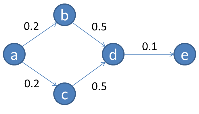
For our example we use the toy social network in Fig. 1. In this example, there are five users , adoption probabilities and propagation probabilities (on edges) are reported in the figure. Let us consider two ways of allocating discounts to users. The first one is , i.e., allocating to : under , accepts the offer with probability ; and will be influenced with probability ; will be influenced with probability ; will be influenced with probability . The expected cascade size under is . Consider the second allocation , i.e., allocation to and : under , (resp. ) accepts the offer with probability (resp. ); is influenced with probability ; is influenced with probability ; is influenced with probability . The expected cascade size under is . Therefore leads to larger expected cascade than .
4.2 Adaptive Setting
Different from the previous setting where we have to commit the set of initial users and corresponding discounts all at once in advance, under the adaptive setting, the decision process is performed in a sequential manner. Each initial user that is probed provides her feedback on the discount rate, or, in other words, reveals whether or not she will adopt the discount. The action taken in each step depends on the actual cascade that happens in the previous steps and remaining budget. Therefore any feasible solutions are now policies instead of a fixed configuration.
Definition 4.1 (Seeding Realization)
For every configuration , is either in “accept” state () or in “reject” state (), describing whether accepts or not. We represent the state of the seeding stage using function , called seeding realization.
Definition 4.2 (Diffusion Realization)
For every edge , it is either in “live” state or in “blocked” state. (describing whether the propagation through is a success or not). We represent the state of the diffusion stage using function , called diffusion realization.
After probing a s-d pair we are able to obtain the seeding realization, i.e., decides wether or not to accept . If decides to accept the discount, we further get to see the realization of the diffusion stage, i.e., the status (live or dead) of all edges exiting , for all nodes reachable from via live edges social network i.e., reachable from under . After each attempt of probing, our observations so far can be represented as a partial realization .
Definition 4.3 (Adaptive Policy)
We define our adaptive policy , which is a function from the current “observation” to , specifying which s-d pair to pick next under a particular set of observations, e.g., chooses s-d pair given s-d pairs have been probed so far, and the resulting cascade.
Assume there is a known prior probability distribution (and resp.) over seeding realizations (and diffusion realizations resp.). Given a realization , let denote all s-d pairs picked by under , and denote the total amount of discount that have been delivered by under . The expected cascade of a policy is where the expectation is taken with respect to and . The goal of the Adaptive Coupon Distribution (ACD) problem is to find a policy such that
ACD:
Maximize
subject to:
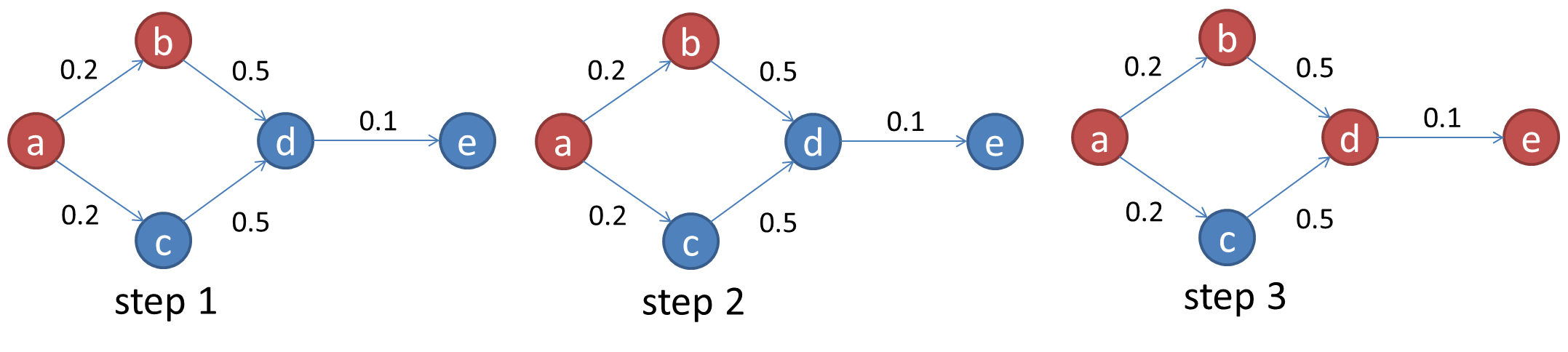
For our example we use the toy social network in Fig. 2, all settings of this example are identical to Fig. 1. Consider a possible adaptive policy as follows: We first probe , that is offering discount to user , and observe the following partial seeding realization: , i.e., accepts the offer; and partial diffusion realization: and , i.e., user is influenced by , user has not been influenced. In the second step where the remaining budget is 1, we probe , that is offering discount to user and obtain the following seeding realization: , i.e., user does not accept the offer. In the third step where the remaining budget is still 1, we probe , that is offering discount to user , and observe that , i.e., user has accepted this offer, and , i.e., has been influenced by . Thus the number of influenced users is 4.
5 Non-Adaptive Discount Allocation Problem
In this section, we study non-adaptive discount allocation problem. Our main idea is to prove that the influence function is monotone and submodular, exploiting these properties, a simple greedy algorithm can achieve approximation ratio.
Definition 5.1 (Submodular function)
Consider an arbitrary function that maps subsets of a finite ground set to non-negative real numbers. We say that is submodular if it satisfies a natural “diminishing returns” property: the marginal gain from adding an element to a set is at least as high as the marginal gain from adding the same element to a superset of . Formally, a submodular function satisfies the follow property: For every with and every , we have that
We say a submodular function is monotone if whenever .
To prove that the influence function is monotone and submodular, we need to focus on the value of , for arbitrary sets and s-d pair . Since the increase of the above expression is very difficult to analyze directly, we take an equivalent view of the cascade process by decomposing it into two realizations:
- 1.
seeding realization . Consider a point in the seeding stage when is probed, i.e, node has been offered discount , accepts offer and becomes the seed with probability . We can view the outcome of this random event as being determined by comparing with a random number that is uniformly selected from : if , then is declared to be valid under .
- 2.
diffusion realization . We follow the same approach introduced in (Kempe et al. 2003) to model the diffusion dynamics. In particular, for each edge in the graph, a coin of bias is flipped at the very beginning of the process. The edges for which the coin flip indicated an successful activation are declared to be live in ; the remaining edges are declared to be blocked in . As described in detail later, a user is influenced if it can be reached from some seed through a path consisting of live edges.
Similar to the diffusion realization, where the coin can be flipped at the beginning of the process, the seeding realization can also be performed ahead of the actual seeding stage. In particular, for each node , a random number is uniformly selected from : if there exists a with and , then is declared to be live under discount . Given a configuration and a seeding realization , we say a node is live under and if and only if there exists such that is live with discount . With both seeding and diffusion realizations are performed in advance, it is easy to determine the subset of nodes that can be influenced at the end of the cascade process:
Claim 1
Given a configuration and realization , a node ends up influenced if and only if is live or there is a path from some live node to consisting entirely of live edges.
Theorem 5.2
The influence function is submodular.
Proof: We first prove that for each fixed realization , the function is submodular. We use to denote the (deterministic) influence function under a fixed realization . Let and be two configurations such that , and consider the value , this is the number of users that can be reached by live users in but not in . This number is at least as large as the number of users that can be reached by live users in but not in . It implies that Then due to the fact that a non-negative linear combination of submodular functions is also submodular, is also submodular.
We next propose a hill-climbing algorithm (Algorithm 1) with a constant approximation ratio. Our algorithm computes two candidate sets: The first candidate set contains a single s-d pair which can maximize the expected cascade: where ; the second candidate solution is computed by greedy algorithm in which we always add that can maximize the expected incremental marginal gain with respect to the discount rate: until the budget constraint is violated. Then we choose the better one as the final output . It was worth noting that computing is #P-hard (Chen et al. 2010), and is typically approximated by numerous Monte Carlo simulations, however, running such simulations are extremely time consuming. Instead, we can leverage a FPRAS (Fully Polynomial Randomized Approximation Scheme) (Long and Wong 2011) for estimating . Based on (Khuller et al. 1999) and the submodularity of , we can prove that our greedy algorithm achieves -approximation.
Theorem 5.3
Algorithm 1 achieves approximation ratio .
6 Adaptive Discount Allocation Problem
We next study the adaptive discount allocation problem. In the rest of this paper, let (resp. ), as a shorthand notation for (resp. ), denote the expected cascade of under a fixed seeding realization (resp. a fixed diffusion realization ).
6.1 Greedy Policy
We first propose a adaptive greedy policy with bounded approximation ratio.
6.1.1 Policy Description
Our greedy policy is performed in a sequential manner as follows: In each round, we probe the s-d pair, say , that maximizes ratio of conditional expected marginal benefit to cost. If accepts , we deduct the discount from the budget and remove from consideration in the following rounds. Otherwise, if turns down the discount, we simply discard and move to the next round. This process iterates until either the budget is used up or all nodes have been probed at the highest discount rate. The detailed description is listed in Algorithm 2: Given partial diffusion realization , let denote all influenced users under , we use to denote the induced graph of . Let denote the expected marginal benefit of in conditioned on has become the seed. At beginning of each round, we check whether or not there exists such that . If so, probe subject to . Depending on the response from the , we either commit and deduct from the remaining budget or skip to the next round.
We next walk through this greedy policy using Fig. 2. We first probe since it has the highest benefit-to-cost ratio . We observe that accepts the offer and successfully influenced . Conditioned on the above observation, we next probe because it has the highest benefit-to-cost ratio in , and we observe that turns down the offer. Then we probe which has the highest benefit-to-cost ratio in , and observe that has accepted the offer and successfully influenced .
6.1.2 Performance Analysis
We first study a relaxed version of ADA by assuming that the seeding realization is pre-known. Given a seeding realization , each node is associated with a minimum discount at which can become the seed. If will never become the seed under , then . Since it is meaningless to probe a user with any discount lower or higher than , we use to denote the refined solution space under this relaxed setting. Consider a greedy policy as follows: In each round, update the partial diffusion realization , and probe that maximizes . This process iterates until either the budget is used up or all users have been probed.
Lemma 6.1
Under the relaxed setting, given any seeding realization , the greedy policy obtains at least of the value of the best policy .
Proof: Consider two types of seeding realizations depending on the output of : 1. : all users except those whose minimum discount is have become the seeds; 2. : there exists some user with finite minimum discount that can not be included in the solution due to limited budget.
The first case is trivial, because both and must select all possible seeds,
| (1) |
We next focus on the second case: In Theorem 26 (Golovin and Krause 2011), it has been proved that
where denotes the greedy policy with expected budget and denotes the best policy with expected budget . The above result is applicable to the traditional influence maximization problem without considering seeding stage. Taking seeding stage into account, it is easy to extend this result to show that and , this is because the actual cost of is lower bounded by , and the actual cost of is upper bounded by . It follows that
| (2) |
Eqs. (1) and (2) together imply that, for all seeding realization , we have
Surprisingly, we next show that given any realization , the outputs of and are identical.
Lemma 6.2
Given any realization , the outputs of and are identical.
Proof: Recall that under , we probe in each round. Depending on the response from the , we either commit or skip to the next round. We next show that by following , if accepts , then , i.e., will never probe a user with discount higher than her minimum discount. First, it is trivial to verify due to the definition of . We can also prove that otherwise, we can probe with discount which is lower than , leading to higher benefit-to-cost ratio. This contradicts to the assumption that .
We are now ready to prove that the outputs of and are identical. Let denote the first seeds committed by , we prove this result through induction on . The basic case when , i.e., is trivial. As proved above, when accepts , we have . Therefore, the first seed that and commit must be some user that maximizes . Assume by contradiction that commits some user other than , then probing with discount less than or equal to leads to a higher benefit-to-cost ratio. This causes contradiction to the design of . Assume the first users committed by and are identical, we next prove that the -th seed is also identical. Given the partial observation after the first seeds have been committed, the next s-d pair that commits must be some that maximizes , otherwise, probing with discount less than or equal to leads to a higher benefit-to-cost ratio. Therefore, and commit the same set of seeds. This finishes the proof of this lemma.
Theorem 6.3
The greedy policy obtains at least of the value of the best policy .
Proof: We have proved that for all . Based on the definition of , we have . Thus,
Then together with Lemma 6.2, we have
It follows that
This finishes the proof of this theorem.
We observe that the above greedy heuristic has an unbounded approximation ratio in the worst case. Consider, for example, a network consists of nodes: one isolated node and a clique with size . There are two discount rates , and budget is . We further set , and . Assume and . By following the heuristics, we will provide discount to , reaching user in expectation. However, the best strategy is to provide discount to any user except , reaching cascade in expectation. Thus the approximation ratio in this case is as large as .
6.2 Enhanced Greedy Policy
We next show that a small modification to the heuristic can achieve an approximation ratio independent of . Our policy (Algorithm 3) first computes two candidate solutions: The first candidate solution contains a single node which can maximize the expected cascade given that has become the seed: ; the second candidate solution is computed by the greedy policy. Then we choose the one that leads to larger expected cascade as the final solution.
Theorem 6.4
Let and denote the highest discount rate, our enhanced greedy policy obtains at least of the value of the best policy for the Adaptive Coupon Distribution problem with the independent cascade model.
Proof: Similar to proof of Theorem 6.3, we consider two types of realizations and .
We first prove that the following equality holds under : . This is because and must select the same set of seeds due to the definition of . It follows that
| (3) |
Next, consider , we have
| (4) |
The first inequality is due to the adaptive submodularity of , and the second inequality is based on Theorem 6.3. Eqs. (1) and (2) together imply that, under any realization :
It follows that
We further have
Then
Corollary 6.5
Assume , the enhanced policy obtains at least of the value of the best policy for the Adaptive Discount Allocation problem with the independent cascade model.
To further enhance the performance of Algorithm 3, we develop another heuristic as listed Algorithm 4. Algorithm 4 is a natural extension of Algorithm 3: In case does not accept , we remove from consideration of initial nodes and apply Algorithm 3 to the remaining nodes. Otherwise, if accepts , we update the budget and diffusion realization, and apply Algorithm 3 to the remaining graph subject to updated budget. Clearly, the cascade gained from this heuristic is no smaller than the one gained from Algorithm 3, thus we have
Theorem 6.6
Algorithm 4 obtains at least of the value of the best policy for the Adaptive Discount Allocation problem with the independent cascade model.
References
- Badanidiyuru et al. (2016) Badanidiyuru, Ashwinkumar, Christos Papadimitriou, Aviad Rubinstein, Lior Seeman, Yaron Singer. 2016. Locally adaptive optimization: adaptive seeding for monotone submodular functions. Proceedings of the Twenty-Seventh Annual ACM-SIAM Symposium on Discrete Algorithms. SIAM, 414–429.
- Brennan (1995) Brennan, Mike. 1995. Constructing demand curves from purchase probability data: an application of the juster scale. Marketing Bulletin 6 1–58.
- Chen et al. (2013) Chen, Wei, Laks VS Lakshmanan, Carlos Castillo. 2013. Information and influence propagation in social networks. Synthesis Lectures on Data Management 5 1–177.
- Chen et al. (2010) Chen, Wei, Chi Wang, Yajun Wang. 2010. Scalable influence maximization for prevalent viral marketing in large-scale social networks. Proceedings of the 16th ACM SIGKDD international conference on Knowledge discovery and data mining. ACM, 1029–1038.
- Chen et al. (2009) Chen, Wei, Yajun Wang, Siyu Yang. 2009. Efficient influence maximization in social networks. Proceedings of the 15th ACM SIGKDD international conference on Knowledge discovery and data mining. ACM, 199–208.
- Cohen et al. (2014) Cohen, Edith, Daniel Delling, Thomas Pajor, Renato F Werneck. 2014. Sketch-based influence maximization and computation: Scaling up with guarantees. Proceedings of the 23rd ACM International Conference on Conference on Information and Knowledge Management. ACM, 629–638.
- Domingos and Richardson (2001) Domingos, Pedro, Matt Richardson. 2001. Mining the network value of customers. Proceedings of the seventh ACM SIGKDD international conference on Knowledge discovery and data mining. ACM, 57–66.
- Eftekhar et al. (2013) Eftekhar, Milad, Yashar Ganjali, Nick Koudas. 2013. Information cascade at group scale. Proceedings of the 19th ACM SIGKDD international conference on Knowledge discovery and data mining. ACM, 401–409.
- Golovin and Krause (2011) Golovin, Daniel, Andreas Krause. 2011. Adaptive submodularity: Theory and applications in active learning and stochastic optimization. Journal of Artificial Intelligence Research 427–486.
- Kempe et al. (2003) Kempe, David, Jon Kleinberg, Éva Tardos. 2003. Maximizing the spread of influence through a social network. Proceedings of the ninth ACM SIGKDD international conference on Knowledge discovery and data mining. ACM, 137–146.
- Khuller et al. (1999) Khuller, Samir, Anna Moss, Joseph Seffi Naor. 1999. The budgeted maximum coverage problem. Information Processing Letters 70 39–45.
- Leskovec et al. (2007) Leskovec, Jure, Andreas Krause, Carlos Guestrin, Christos Faloutsos, Jeanne VanBriesen, Natalie Glance. 2007. Cost-effective outbreak detection in networks. Proceedings of the 13th ACM SIGKDD international conference on Knowledge discovery and data mining. ACM, 420–429.
- Long and Wong (2011) Long, Cheng, Raymond Chi-Wing Wong. 2011. Minimizing seed set for viral marketing. 2011 IEEE 11th International Conference on Data Mining. IEEE, 427–436.
- Suh et al. (2004) Suh, Euiho, Seungjae Lim, Hyunseok Hwang, Suyeon Kim. 2004. A prediction model for the purchase probability of anonymous customers to support real time web marketing: a case study. Expert Systems with Applications 27 245–255.
- Yang et al. (2016) Yang, Yu, Xiangbo Mao, Jian Pei, Xiaofei He. 2016. Continuous influence maximization: What discounts should we offer to social network users? Proceedings of the 2016 ACM SIGMOD International Conference on Management of Data. ACM.