Modeling Group Dynamics Using Probabilistic Tensor Decompositions
Abstract
We propose a probabilistic modeling framework for learning the dynamic patterns in the collective behaviors of social agents and developing profiles for different behavioral groups, using data collected from multiple information sources. The proposed model is based on a hierarchical Bayesian process, in which each observation is a finite mixture of an set of latent groups and the mixture proportions (i.e., group probabilities) are drawn randomly. Each group is associated with some distributions over a finite set of outcomes. Moreover, as time evolves, the structure of these groups also changes; we model the change in the group structure by a hidden Markov model (HMM) with a fixed transition probability. We present an efficient inference method based on tensor decompositions and the expectation-maximization (EM) algorithm for parameter estimation.
I introduction
In this paper, we consider the problem of modeling discrete social network data and learning the underlying group dynamics. The goal is to develop probabilistic profiles of large collections of data while preserving the essential temporal relationships that provide insights for various applications of interest. For example, in social network analysis, we want to analyze relationships between social agents and their behaviors over time and on various social media sites (i.e., Facebook, Twitter, Instagram, Google+, etc.). In web advertising analysis, we want to analyze the relationships between customers and the types of products they buy from different shopping sites to capture customers’ buying behaviors and learn the intrinsic factors that effect their buying decision process. In the study of scientific collaboration, using co-authorship networks from multiple journals on related subjects, one can analyze relationships between subjects and authors. This will, in turn, allow us to identify individual authors’ area of expertise and potential research directions.
In the past few years, much effort has been devoted in the literature to develop models and algorithms that can efficiently extract the hidden groups/communities of a society. Generally speaking, there are two types of learning approaches. One approach starts by constructing networks that describe relationships or interactions between agents in a social setting; see [1]. The proposed algorithms focus on partitioning the graph into disjoint or overlapping subgraphs to reflect some of the shared features of the groups. The second approach focuses on extracting relevant information from data. For instance, the classical K-means clustering [2, 3, 4] seeks to partition columns of a data matrix by minimizing the sum of squared distances of the data points to their respective cluster centroids. Co-clustering [5] seeks to simultaneously partition rows and columns of a data matrix to form coherent groups, also known as co-clusters. Moreover, the study of multi-way clustering goes beyond pairwise relationship; it seeks to find group structures in a multi-dimensional array via tensor decompositions [6]. Recently, tensor decompositions have also been applied to statistical relational learning as a new approach to infer the structure of a probabilistic graphical model [7, 6, 8]. The latent Dirichlet allocation (LDA) model is another statistical approach for modeling collections of discrete data, such as document classification. It assumes that the words in a document are generated based on a mixture model. Specifically, it emphasizes that each documents contain multiple topics and the words in the document were drawn from these topics in proportion to the topic distribution of the document.
It is worth noting that some of the above-mentioned algorithms for extracting group information assume that the data are from a single source and most of these algorithms do not deal with the problem when the group structure changes over time. Thus, the work that we discuss in this paper focuses on developing a modeling framework for dynamically fusing data from multiple related information sources, as well as learning the group dynamics.
There are several reasons why one should be interested in extracting group information from multiple sources and characterizing patterns of temporal dynamics in different groups. First, in today’s highly computerized environment, large amounts of data are created every second from multiple sources that often share certain dependencies (e.g., mobile phones, SMS, GPS locator, emails, tweets, social networking sites, etc.). It makes sense to fuse data from all relevant information sources for joint analysis. Second, information collected from multiple sources can facilitate in accurately inferring the latent structure of the data. Indeed, many machine learning tasks, such as classification, regression and clustering, can significantly improve their performance if information from multiple sources can be property integrated. Finally, understanding the dependency patterns over time and across multi-source data can be extremely beneficial in many science and engineering applications. In the context of social network analysis, each group can be identified by its membership and the specific actions that the members are likely to perform over time. Then the group probabilities provide an explicit representation of each social media site, which in turn, helps us determine the distances between these social media sites. In the study of scientific collaboration, one can analyze relationships between subjects and authors to identify groups with different research focus. Contrary to the graph-based model, each author may probabilistically belong to several communities (or subject group). Intuitively, an author’s contribution to a community is proportional to the number of publications that he/she has published in these groups. However, estimating contribution by only publication count may be misleading. For example, it is quite possible that one has published less papers in one community turns out to have more contribution in that subject group because of the intrinsic characteristics of the group, such as the rate of publication, number of authors in the group, etc.
I-A Contributions
While the main focus of most of the existing works is to extract group information from a single source in a static model, it is also important to consider fusing information from multiple information sources and over time. Our previous work [9] provides a probabilistic modeling framework for extracting dynamic patterns from multi-source data. This paper is an extension of the work and it incorporates an efficient filter-based expectation-maximization (EM) learning method for performing parameter estimation on both synthetic data and real data. Specifically, we model the dynamics of a group by a hidden Markov model (HMM) and demonstrate how one can make use of a higher-order tensor [10, 11, 12] (i.e., a multi-dimensional array) as an appropriate mathematical abstraction for the probabilistic graphical model [13, 14, 15] that represents the conditional independence structure between latent variables.
I-B Paper Organization
The rest of the paper is organized as follows. In Section II, we review the connection between graphical models and tensor decompositions, and explain how tensor decomposition can be used to transform a graphical model into a structurally simpler inference model. In Section III, we extend the model and formulate a dynamic tensor decomposition model for learning the low-dimensional structure from observed high-dimensional multi-source data. In Section VI, we show the performance of the proposed framework for modeling group dynamics via simulations.
II Mapping a Graphical Model into a Low-rank Tensor Decomposition: A Static Model
In this section, groups and basic group features are defined. Their relationship with the LDA model is explained, followed by a description of how information from multiple information sources can be used to predict intrinsic group structure via tensor decomposition.
II-A Latent Groups
Suppose there are information sources, i.e., . Examples include various social network websites in social network analysis, different shopping sites in the analysis of web advertisement, different subjects/journals in the study of scientific collaboration, etc.. Given each source, we observe joint occurrences of two events and , with discrete outcomes in the finite sets and , respectively. One example is that of a person posting a picture. Here event is that a person is active and event is that a picture is posted. Other examples include a customer buying a particular product, a researcher collaborating with another researcher, etc.. For simplicity, we only consider the case of observing joint occurrences of two events and . However, the approach can be generalized to a larger number of events with a higher dimensions.
Let the tensor be such that its element denotes the joint probability that events are observed in the information source:
| (1) |
Given , if two events and are independent, then .
In practice, however, events and , conditioned on a particular information source , are often dependent. For instance, in computing the probability of an agent posting a photo on Facebook, the agent and the particular activity (i.e., posting a photo) are two dependent variables. Similar arguments can be made for the shopping behavior of a customer and co-authoring a paper on a specific subject.
Given that and are dependent, let us assume that the information source itself is an event, determined by a latent variable , drawn from the groups such that conditioned on the groups, and are independent. That is, probability mass functions (PMFs) of and are conditionally independent given the group : and . Subsequently, Eqn. (1) becomes
| (2) |
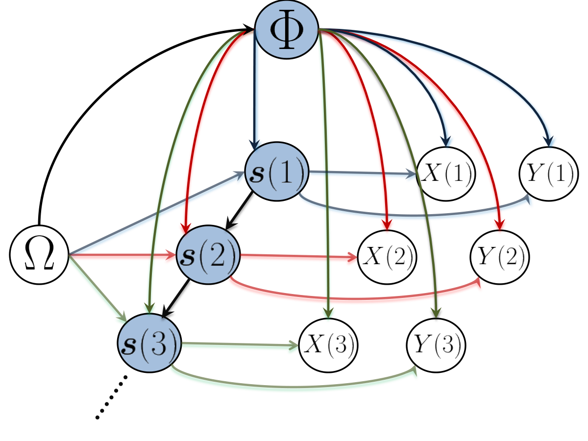
where represent group probabilities for source and they sum up to . Here we assume that they are drawn randomly from a fixed distribution. Fig. 1 shows its corresponding graphical model.

Indeed, the above description is analogous to the LDA model, a generative model describing the generation of words in a collection of documents. That is, for a given information source , a group distribution is drawn from a fixed distribution. (In the LDA model, this fixed distribution is modeled as a Dirichlet distribution). Let be the number of joint events to be sampled. For each of the samples, one of the groups is probabilistically drawn from the group probabilities . Given the group , events and are drawn independently from distributions and respectively.
Several simplifying assumptions are made in this model. First, the number of groups is assumed known and fixed. Second, the group features are represented by the probability vectors and , where and , respectively. For now, we treat them as fixed quantities for the given group. Lastly, we treat as an ancillary variable and its value is generally known for a given dataset. Our goal is to estimate the latent groups from the information sources and the tensor decomposition offers a way to estimate these group features.
II-B Tensor Decompositions
Given the group features and for , it follows from (2) that the frontal slice of the tensor can be written as
| (3) |
where denotes the group probability. Furthermore, the above expression is equivalent to the following PARAFAC tensor decomposition: let be the column of the matrix , then the given tensor can be decomposed into
| (4) |
under the constraint that , and , where the symbol denotes the outer-product.
III Clustering Behaviors in Dynamic Models
The static model in (3) and (4) assumes that for any given group , the PMFs of and are fixed quantities. Information from multiple sources can be fused together to extract group features using the tensor decomposition. However, in many applications, group features often evolve over time; thus it is also important to understand how the group patterns change over time and across different information sources.
III-A A Dynamic Model
We model the dynamics of each information source by a Markov model and assume the following generative process for each information source :
- 1.
Choose group probabilities from some distribution
- 2.
For each timestamp :
- (a)
Choose the number of joint events to be sampled:
- (b)
Choose a Markov state from the distribution for all
- (c)
For each of the sampled joint events where :
- i.
Choose a group
- ii.
Choose events and independently from multinomial distributions and , respectively.
- i.
- (a)
Several assumptions are made. First, the number of groups and the number of Markov states in each group are assumed known and fixed. Second, the group features evolve over time and we model it as a Markov process with a fixed group transition matrix . Finally, the Poisson assumption for generating is not critical to parameter estimation and its value is generally known given a dataset.
III-B Hidden Markov Models
Assume that the group probability is nonzero, at each time , we associate to a state in a hidden Markov model (HMM), where denotes the canonical base vector (with one in the component and zero elsewhere) and denotes the total number of states. Given the past states, the Markov property of a state transition implies
i.e., the conditional distribution of the state at time depends only on the state at the previous time and not on the sequence of states that preceded it. For all the transition probability from state to state is time-invariant. The matrix with defines the transition matrix of the Markov chain and is row-stochastic. Moreover, given the state , the probability distribution of the state can be written as
| (5) |
Define . It follows from (5) that the expectation of conditioned on the past states equals zero: . This property will be used in a later section to derive a recursive state estimation filter.
The particular choice of using the coordinate vectors to represent states in a HMM is attractive for several reason: 1) any function of the state can be written as a linear function of coordinate vectors (and hence it commutes with the expectation operator); 2) the expected value of equals the probability distribution of the state, i.e., . This simplifies the state estimation of the Markov chain; see Section V for a detailed discussion.
III-C Tensor Representations
Under the proposed dynamic model, given a group , the transition probability is independent of and there exist two dictionaries of PMFs: and for the two random variables and , respectively; the column of and correspond to the PMFs of and , respectively, when is in the state . Hence, the frontal slice of the tensor obeys the following expression:
| (6) |
Fig. 2 shows the graphical model corresponding to the dynamic tensor . Importantly, in contrast to the static model in (3) where the group features are identified by the fixed PMFs and , the dynamic model assumes that given , the group features dynamically have the same set of PMFs for the variables and with the same transition probability.
Define to be the following matrix product:
| (7) |
It follows from (6) that the decomposition of the time-varying tensor can be written as
| (8) |
where , and denote the columns of matrices , and , respectively. Note that the dynamics of the system is given by the vector, while the dictionaries of group properties are fixed.
III-D Sampling Distribution: the Multinomial Case
Recall from the generative process where at each time period, we sample occurrences of the joint events. Let be a counting matrix whose element represents the number of times the pair is observed from during the time interval; -norm of equals . Moreover, the the counting matrix follows a multinomial distribution with parameter and .
Using the Central Limit Theorem [16], for sufficiently large, one can approximate the multinomial distribution with the following multivariate normal distribution: where the mean is and the covariance is a function of the mean:
| (9) |
Note that the covariance matrix is not full rank; the multivariate normal dsitribution is degerenate. We say that the normalized observation follows a degenerate normal distribution, whose density is given by
| (10) |
where is the generalized inverse of given in (9) and denotes the pseudo-determinant.
Importantly, computing the generalized inverse of the covariance matrxi can be computationally infeasible for large data sets. The following lemma gives explicit expressions for the generalized inverse and the pseudo-determinant.
Lemma 1
Given that is an -dimensional probability vector (i.e., and ), let be the indicator vector whose element equals if its corresponding element in is positive and otherwise. Let denote a -dimentional vector such that its element equals when and 0 otherwise. The pseudo-determinant and the generalized inverse of are given by
where .
In summary, given the normalized observations , we have
| (11) | ||||
where the noise is degenerate normal distributed; the matrix is a function of the mean vector .
IV Maximum Likelihood Inference
Let and be the sets of unknown parameters. Given the normalized observation tensors and the count numbers for all , the likelihood function is given by
| (12) |
under the constraint that , are non-negative row-stochastic and , are non-negative column-stochastic.
For the ease of notation, let be an array of indices of the individual Markov states in their corresponding groups, i.e., and . Let with be a sequence of the index array corresponding to all the possible combinations of the Markov states; we denote the set of all . We apply the expectation-maximization (EM) algorithm to find the maximum likelihood estimators by iteratively maximizing the following -function:
where is a constant and
| (13) | ||||
| (14) |
in which denotes the expectation under the probability measure with model parameters equal to the estimated values (i.e., and ), is the probability density function given in (10) and denotes the mean of the Gaussian observation from source given , that is,
| (15) |
IV-A E-Step: Computing the -function
It follows from the techniques in [17, 18], the following processes are defined to compute the -function:
| (16) | ||||
| (17) | ||||
| (18) |
In particular, the term defines the number of jumps from state to state for the source and the group ; defines the combined occupation time for source in the given Markov states associated with the index set . The term in Eqn. (18) takes one of the three forms:
| (19) | ||||
| (20) | ||||
| (21) |
with and denotes the Hadamard product.
IV-B M-step: Updating parameters in
The estimate of can be updated by maximizing , under the constraint that each is a row stochastic matrix. Using the method of Lagrange multipliers and equating the derivative to yields
| (22) |
It follows from the -function that the parameters in can be estimated by minimizing the following cost function:
| (23) |
Gradient algorithm is used to update each of the parameters in the set . The gradient of the cost function with respective to any parameter can be written as
| (24) |
where is the Jacobian matrix of with respect to the parameter and
| (25) |
in which constants and are given by
| (26) | ||||
| (27) |
and , , represent the following conditional expectations:
| (28) | ||||
| (29) | ||||
| (30) | ||||
| (31) |
The above conditional expectations can be computed in the -step via filter-based learning, as discussed in the next section.
Algorithm 1 summarizes the main steps for parameter estimation. The algorithm starts with initial estimates of the parameters . The specific choice of the initial estimates and model order selection rule will be discussed in Section VI where numerical results are reported. The (generalized) EM algorithm alternates between the E-step, which computes the set of conditional expectations in the -function, and a M-step, which updates the parameters by maximizing the -function. In particular, the transition matrices for all can be updated using (22). Since there does not exist a closed-form solution for parameters , an iterative projected gradient algorithm is used. Specifically, denotes the projection function that projects columns of the input matrix onto their corresponding canonical simplexes. The expression inside the projection function is a regular gradient descent step in which the stepsize is set to be sufficiently small and proportional to the parameters to be updated.
V Filter-Based Learning
In this section, we introduce a filter-based algorithm for learning the conditional expectation that are required in the evaluation of the -function in the E-step. Contrary to the traditional forward-backward algorithm, the filter-based algorithm does not required extra storage for the intermediate quantities. The filtering processes for different terms in the E-step is independent, thus making parallel processing possible if needed.
V-A Filter-Based State Estimation
This section investigate the estimation of the state distribution for all and . The key is to introduce a measure transformation, which is defined by the likelihood ratio
| (32) |
where the numerator represents the probability distribution of the Gaussian observation given in (10) and denotes the probability distribution of the observation for . Thus, given and the function in (20), it follows from Lemma 1 that the computation of the likelihood ratio is reduced to the following expression:
| (33) |
where . Let
| (34) |
be the product of the transformation up to time . The conditional Bayes’ Theorem yields
| (35) |
Hence, given the current estimates , the state distribution for source can be described by normalizing the vector . Our goal is to derived a recursive expression for computing this un-normalized state distribution.
Define . Let such that if and only if its element of equals . Then one can derive the following recursive relation: (see Appendix)
| (36) | ||||
| (37) |
Then it follows from (35) that the probability distribution of the Markov state is given by
| (38) |
and the estimated state of source in group at time is simply the one that corresponds to the highest likelihood.
Similarly, one can also compute the probability distribution of the set of Markov states. Given the sequence of index arrays and the transition matrices for all , one can construct another hidden Markov model in which denotes the state at time and denotes the tranition matrix. Each state is associated to its corresponding element in the sequence and the element of the transition matrix represents the probability of transitioning from state to state . Let . Following a derivation similar to that in (36), it can be shown that
| (39) |
where is given by the following recursive expression:
| (40) | ||||
| (41) |
We are now ready to computer the conditional expectations in the -function.
V-B Filter-Based Computation of the -Function
Recall from Section IV-A that the computation of the -function is reduced to computing the following conditional expectations: , and . The first term is used to estimate the transition matrix for all as given in (22). The second and the third terms the gradient of the cost function with respect to the parameters in the set ; see Eqn. (25) and (28) - (31). In this section, we will discuss how to recursively compute these terms using the technique introduced in the previous section.
Define . Then at time , we have
| (42) |
Note that the term in the denominator can be computed recursively using (36). Following a similar procedure as in (36), one can derive the following recursive expression:
| (43) | ||||
Similarly, let and , respectively, where denotes the element of . Then for , we have . Thus it can be shown that
| (44) | ||||
| (45) |
where the term in the denominator is given by the recursive expression in (40) and
| (46) | ||||
| (47) | ||||
Using the filters derived in (43), (46), (47), one can then evaluate the -function and perform parameter update, as shown in Algorithm 1.
VI Numerical Result
In this section, we present numerical results using both synthetic data and real data. We use K-means clustering to initilaize the parameters. It is an extremely fast algorithm and has no hyper-parameter to tune beyond setting the model orders.
VI-A Synthetic Datasets
Two groups and are generated, thus . The first group has hidden Markov states with a fixed transition matrix while the second group has hidden Markov states with a fixed transition matrix . information sources are generated; each is associated with some group distribution , uniformly sampled over a -dimensional simplex. Moreover, for each latent group , a pair of dictionaries and are generated; each column in and represents a discrete probability vector, such that the resulting tensor in (8) at each time satisfies the sufficient condition for a unique decomposition [19, 20, 21]. Observations for are generated according to the model described in Section III. In the simulation, we set the number of sampled events to be a constant for all and all , here we simply denote it as . Recall that larger value of implies that observations are less noisy.
The performance of the learning algorithm is measured by the mean-squared-error (MSE) between the recovered (or estimated) tensors and the observations :
Fig. 3 shows the performance of the learning algorithm for sources and observation time as the sample size increase. For each value of , the algorithm is run times; each with a different set of group probabilities while the group features and are fixed. Observe that the averaged MSE over runs decreases as the sample size increases.

Fig. 4 shows the performance of the learning algorithm for different number of sources, i.e., . Observe that the averaged MSE (over runs) decreases as the number of information sources increases.

Fig. 5 show the performance of the learning algorithm for observations. Observation that averaged MSE (over runs) decreases significantly from to , but there is hardly any improvement from to .

VI-B Synthetic Datasets with Missing Values
This section investigate the robustness of the proposed learning algorithm when there are missing data. Here we assume that the loss is uniformly random over time. The algorithm treats the missing data as zero. Fig. 6 shows the averaged MSE (over runs) for information sources as the percentage of missing data increases. The dotted lines represent the MSE between the recovered tensors and the observed tensors with missing values, while the solid lines represent the MSE between recovered tensors and the original tensors with no missing value. Observed that the recovered tensors are closer to the original tenors than the input tensors with missing values. Moreover, when the percentage of missing data is small, information sources performs better. As the percentage of missing data increases, the advantage of having more sources diminishes.
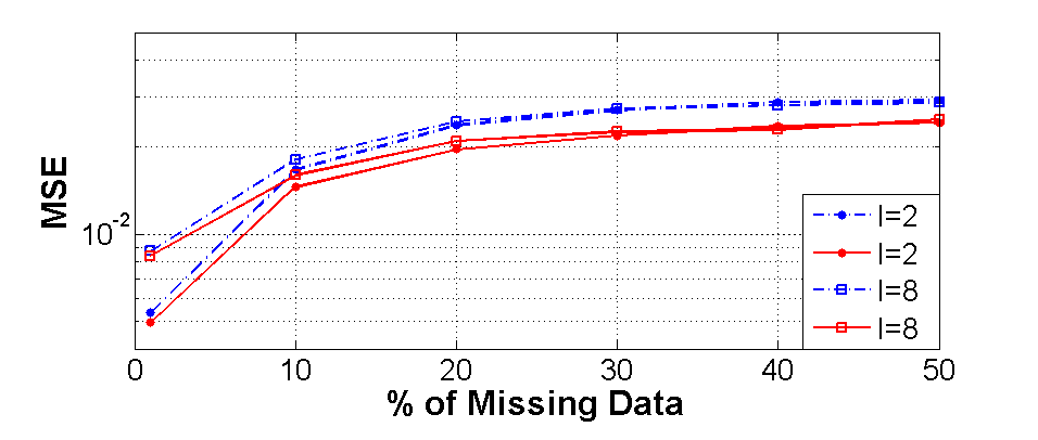
To get a clearer idea of the effects of missing data, Fig. 7 shows the normalized MSE as the percentage of missing data increases. Here we normalized the averaged MSE with missing data (Fig. 6) by the averaged MSE when there is no missing data. Again the dotted line represent the normalized MSE between the recovered tensors and the observed tensors with missing values, and the solid lines represent the normalized MSE between the recovered tensors and the original tensors with no missing value. Observe that the loss in performance is more significant for larger values of .

VI-C APS dataset: Atomic, Molecular and Condense Matter Physics
In this section, we validate the proposed model using the bibliographic database from American Physical Society (APS). Five journals are considered, i.e., PRA, PRB, PRC, PRD and PRE, from the year to the year . We selected three research areas for investigation: (1) Atomic and Molecular Physics; (2) Condensed Matter: Structural, Mechanical and Thermal Properties; (3) Condensed Matter: Electronic Structure, Electrical, Magnetic, and Optical Properties. There are a total of subjects under these research areas. We excluded the subjects that have less than publications for any given sample period because they are likely to increase the variability of the data and decrease the performance of the estimation. Table VI-C lists the resulting subjects and their corresponding Physics and Astronomy Classification Scheme (PACS). Furthermore, we excluded authors who have published less than papers over the years of interest, because authors who has published small number of papers do not provide us with sufficient samples of their co-authors over the years.
| PACS | Subjects | |
|---|---|---|
| 1 | 31 | Electronic structure of atoms and molecules: theory |
| 2 | 32 | Atomic properties and interactions with photons. |
| 3 | 34 | Atomic and molecular collision processes and interactions |
| 4 | 61 | Structure of solids and liquids; crystallography |
| 5 | 63 | Lattice dynamics |
| 6 | 64 | Equations of state, phase equilibria, and phase transitions |
| 7 | 68 | Surfaces and interfaces; thin films and nanosystems (structure and nonelectronic properties) |
| 8 | 71 | Electronic structure of bulk materials |
| 9 | 72 | Electronic transport in condensed matter |
| 10 | 73 | Electronic structure and electrical properties of surfaces, interfaces, thin films, and low-dimensional structures |
| 11 | 74 | Superconductivity |
| 12 | 75 | Magnetic properties and materials |
| 12 | 78 | Optical properties, condensed-matter spectroscopy and other interactions of radiation and particles with condensed matter |
| 14 | 79 | Electron and ion emission by liquids and solids; impact phenomena |
The temporal tensor data are constructed as follows. Each subject is considered as one information source. For each subject and a given time block, we construct a co-authorship network, in which the nodes represent authors and two authors are connected if they have co-authored at least one paper. The strength of their connection is given by the number of papers they’ve collaborated on. Hence, the slice of resulting tensor at time is given by the weighted adjacency matrix of the corresponding co-authorship network, normalized by the sum of the weights of its edges, i.e., the total number of paper published in the respective subject. Each time represents a -year period; thus there are a total of time periods from year to the year .
VI-C1 Model Order Selection and Parameter Initialization
To select an optimal number groups and the number of the Markov states within each group, we use the method proposed by Pham, et.al. in [22], which builds on the -means algorithm. Specifically, we first compute the degree centralities of all the weighted graphes and use them as inputs to the method proposed in [22] to select an optimal number of groups. The -means algorithm is performed to give group labels to the input data points. For the data points of a given group label, we run the method in [22] again to select an optimal number of Markov states for the given group and use -means algorithm to initialize the group dictionary for all the groups . Since the co-authorship network is un-directed, we have . To initialize the group probability matrix , for each subject, we count the group labels of the degree centrality vectors for each group, and assign a higher probability to the group with a higher count number. To avoid getting stuck in a local minimum, several different probability matrices are tested initially and we pick the one that gives the smallest MSE.
VI-C2 Numerical Results
Given the dataset as described earlier, the model selection procedure indicates that there are groups and the numbers of Markov states in the respective groups are and . Fig. 8 shows the evolution of the MSE. Observe that the MSE, which measures the goodness of fit, decreases as the number of maximum likelihood iteration increases. Fig. 9 shows the estimates the group dictionaries. The x-axis represents the authors, the y-axis represents discrete Markov states, and the color represents the participation of the authors given the state in a group. Observe that each group has a set of active authors. There are authors who belong to both groups, authors who only publish in group and authors who only publish in group . Fig. 10 shows the group probability of each of the subjects belonging to group . Observe that the first subjects are similar to each other and subjects are similar to each other. Indeed, it follows from Table VI-C that the first subjects are in the area of atomic and molecular physics while the rest of the subjects are in the area of condense matter. In addition, from the group probabilities shown in Fig. 10, it can be seen that the two groups are very loosely related.


VI-D APS dataset: Elementary Particles and Nuclear Physics
In this section, we investigate the fields of elementary particles and nuclear physics in the APS dataset. It is to be noted that the model order selection protocol returns group on all the subjects unders these two areas. That is, if we consider all the authors who have published more than papers under these two areas, we can not tell these subjects apart; they are closely related.
To obtain a more insightful result, we now consider only the “experts” in the fields, that is, authors who have published more than papers. Then we eliminate the subjects that don’t have sufficient number of publications in any given time period. The resulting subjects of interest are listed in Table VI-D. PACS belong to the area of Elementary Particles and Fields, while PACS belong to the area of Nuclear Physics. The model order selection protocol suggests that there are two groups; the first group has Markov states and the second group has Markov states.
| PACS | Subjects | |
|---|---|---|
| 1 | 11 | Electronic structure of atoms and molecules: theory |
| 2 | 12 | Atomic properties and interactions with photons. |
| 3 | 13 | Atomic and molecular collision processes and interactions |
| 4 | 14 | Structure of solids and liquids; crystallography |
| 5 | 21 | Lattice dynamics |
| 6 | 23 | Equations of state, phase equilibria, and phase transitions |
| 7 | 27 | Surfaces and interfaces; thin films and nanosystems (structure and nonelectronic properties) |
Fig. 11 shows the evolution of the MSE as the number of iterations increases. Observe that the MSE decreases monotonically. Fig. 13 shows the estimated group dictionaries. The color represents individual authors participations’ in their respective groups and for a given state. Observe that each group has a set of active authors. There are authors who only publish in the first group, authors who only publish in the second group, and authors who publish in both groups. Fig. 13 shows the group probabilities of each subject belonging to group . If the threshold for classification is set to be , then it can be seen that the first four subjects form one cluster and they represents subjects in the area of Elementary Particles and Fields, while the last three subjects form the second cluster and they represent Nuclear Physics. In Contrast to Fig. 10 in the previous section, the distances between the group probabilities of different subjects are closer. It implies that these subjects are very much related because authors who publish in the subjects in the area of Elementary Particles and Fields are also likely to publish in the subjects in the area of Nuclear physics.


VII Conclusion
This paper introduced a general modeling framework for learning group dynamics in observed data collected from multiple information sources and over time. The proposed model allows us to analyze relationships between different sources and to make inferences on the temporal patterns of the group behaviors.
VIII Appendix
Derivation of Eqn. (36).
References
- [1] S. Fortunato, “Community detection in graphs,” Physics Reports, vol. 486, no. 3–5, pp. 75 – 174, 2010. [Online]. Available: http://www.sciencedirect.com/science/article/pii/S0370157309002841
- [2] S. Lloyd, “Least squares quantization in PCM,” Information Theory, IEEE Transactions on, vol. 28, no. 2, pp. 129–137, Mar 1982.
- [3] A. Banerjee, S. Merugu, I. S. Dhillon, and J. Ghosh, “Clustering with Bregman divergences,” J. Mach. Learn. Res., vol. 6, pp. 1705–1749, Dec. 2005. [Online]. Available: http://dl.acm.org/citation.cfm?id=1046920.1194902
- [4] K. Chaudhuri and A. McGregor, “Finding metric structure in information theoretic clustering,” Proceedings of the 21st Annual Conference on Computational Learning Theory, pp. 391–402, July 2008.
- [5] A. Banerjee, I. Dhillon, J. Ghosh, S. Merugu, and D. S. Modha, “A generalized maximum entropy approach to Bregman co-clustering and matrix approximation,” J. Mach. Learn. Res., vol. 8, pp. 1919–1986, Dec. 2007. [Online]. Available: http://dl.acm.org/citation.cfm?id=1314498.1314563
- [6] M. Nickel, V. Tresp, and H.-P. Kriegel, “A three-way model for collective learning on multi-relational data,” in Proceedings of the 28th International Conference on Machine Learning (ICML), 2011.
- [7] I. Sutskever, R. Salakhutdinov, and J. B. Tenenbaum, “Modelling relational data using Bayesian clustered tensor factorization,” Adv. Neural Inform. Proc. Sys., 2009.
- [8] L. Song, M. Ishteva, A. Parikh, E. Xing, and H. Park, “Hierarchical tensor decomposition of latent tree graphical models,” in Proceedings of the 30th International Conference on Machine Learning (ICML), 2013.
- [9] L. Li, A. Swami, and A. Scaglione, “Modeling group dynamics using graphical models and tensor decompositions,” in Signal and Information Processing (GlobalSIP), 2014 IEEE Global Conference on, Dec 2014, pp. 793–797.
- [10] L. Tucker, “Some mathematical notes on three-mode factor analysis,” Psychometrika, vol. 31, no. 3, pp. 279–311, 1966.
- [11] R. Bro, “PARAFAC tutorial and applications,” Chemometrics and Intelligent Laboratory Systems, vol. 38, no. 2, pp. 149 – 171, 1997.
- [12] T. G. Kolda and B. W. Bader, “Tensor decompositions and applications,” SIAM Review, vol. 51, no. 3, pp. 455–500, 2009.
- [13] J. Pearl, Probabilistic Reasoning in Intelligent Systems: Networks of Plausible Inference. San Francisco, CA, USA: Morgan Kaufmann Publishers Inc., 1988.
- [14] R. G. Cowell, A. P. Dawid, S. L. Lauritzen, and D. J. Spiegelhalte, Probabilistic Networks and Expert Systems: Exact Computational Methods for Bayesian Networks. Springer-Verlag, New York, 1999.
- [15] M. I. Jordan, “Graphical models,” Statist. Sci., vol. 19, no. 1, pp. 140–155, 2004.
- [16] T. A. Severini, Elements of Distribution Theory. Cambridge University Press, 2012. [Online]. Available: http://EconPapers.repec.org/RePEc:cup:cbooks:9781107630734
- [17] L. Li, “Learning hidden Markov sparse models,” Information Theory and Applications (ITA), 2013.
- [18] L. Li, A. Scaglione, J. H. Manton, and A. Swami, “Hidden Markov sparse models (HMSM) for batch and online dictionary learning,” 2013, submitted to IEEE TPAMI.
- [19] J. B. Kruskal, “Three-way arrays: rank and uniqueness of trilinear decompositions, with application to arithmetic complexity and statistics,” Linear Algebra and its Applications, vol. 18, no. 2, pp. 95 – 138, 1977.
- [20] A. Stegeman and N. D. Sidiropoulos, “On Kruskal’s uniqueness condition for the CANDECOMP/PARAFAC decomposition,” Linear Algebra and its Applications, vol. 420, no. 2–3, pp. 540 – 552, 2007.
- [21] J. Ten Berge and N. Sidiropoulos, “On uniqueness in CANDECOMP/PARAFAC,” Psychometrika, vol. 67, no. 3, pp. 399–409, 2002.
- [22] D. Pham, S. Dimov, and C. Nguyen, “Selection of in k-means clustering,” Mechanical Engineering Science, vol. 219, pp. 103–119, 2004.