Optimal adaptation for early stopping
in statistical inverse problems
Abstract
For linear inverse problems , it is classical to recover the unknown signal by iterative regularisation methods and halt at a data-dependent iteration using some stopping rule, typically based on a discrepancy principle, so that the weak (or prediction) squared-error is controlled. In the context of statistical estimation with stochastic noise , we study oracle adaptation (that is, compared to the best possible stopping iteration) in strong squared-error .
For a residual-based stopping rule oracle adaptation bounds are established for general spectral regularisation methods. The proofs use bias and variance transfer techniques from weak prediction error to strong -error, as well as convexity arguments and concentration bounds for the stochastic part. Adaptive early stopping for the Landweber method is studied in further detail and illustrated numerically.
Key words and Phrases: Linear inverse problems. Early stopping. Discrepancy principle. Adaptive estimation. Oracle inequality. Landweber Iteration.
AMS subject classification: 65J20, 62G05.
1 Introduction and main results
1.1 Motivation
Statistical linear inverse problems
We wish to recover a signal (a function, an image) from noisy data when the observation of the signal is further challenged by the action of a linear operator. As an illustrative example, we consider the model of inverse regression in dimension over . We observe
| (1.1) |
where is the signal of interest, is a bounded linear operator (with a continuous function), is a measurement noise level and are independent standard normal random variables. An idealised version of (1.1) is given by the continuous observation of
| (1.2) |
where is a Gaussian white noise in with noise level
| (1.3) |
For the asymptotics the rigorous statistical equivalence between (1.1) and (1.2) goes back to Brown and Low [8] and was extended to higher dimensions and possibly in Reiß [24]. This setting of statistical inverse problems is classical and has numerous practical applications, see among many other references Mair and Ruymgaart [21], Cohen et al. [11], Bissantz et al. [5] and the survey by Cavalier [9].
Early stopping and regularization
Most implemented estimation or recovery methods for are based on a combination of discretisation and iterative inversion or regularisation. Start with an approximation space with . First, suppose that (1.1) is observed without noise, i.e., . An approximation for is then obtained by minimising the criterion
Using gradient descent (also called Landweber iteration in this context), we obtain the fixed point iteration for :
| (1.4) |
If , we have the convergence as .
The same program applies when the data are noisy: we fix a large approximation space and transfer our data into the approximating linear model
| (1.5) |
with , and , with obvious matrix-vector notation. In formal analogy with (1.4) we obtain a sequence of iterations
| (1.6) |
The presence of a noise term generates a classical conflict as grows: the iterates are ordered with decreasing bias and increasing variance , where denotes expectation. Thus, early stopping at some iteration serves as a regularisation method which simultaneously reduces numerical and statistical complexity at the cost of a bias term.
More generally, spectral regularisation methods for linear inverse problems take the form , where is a one-parameter family of functions satisfying certain generic conditions, see Engl et al. [13]. In this parametrisation the limit corresponds to less regularisation, with being the unregularised inverse. In this paper, we will consider such general regularisation schemes using the reparametrisation ; hence, a larger regularisation parameter , to be interpreted as computational time, indicates less regularisation (or a larger variance) and .
Regularisation methods can be iterative or not, but it is common that the regularisation parameter is chosen from a fixed in advance grid , as , which we still refer to as “iterations”. Conversely, any regularisation method defined only on a discrete grid, such as Landweber iteration, can be extended to a continuous regularisation method by appropriate interpolation, see also Remark 2.2 on the discretisation error below. We note that even for methods that are not intrinsically iterative (for instance Tikhonov regularisation ), computing the estimates for larger is generally more resource-intensive since this computation is often numerically less stable.
1.2 Adaptivity, oracle approach and early stopping
There are several ways to choose from the data to try to achieve close to optimal performance. Recent results are formulated within the oracle approach, comparing the error of to the minimal error among . An idealized oracle inequality would take the form
| (1.7) |
where indicates inequality up to a constant. Such an inequality can be seen as a convenient way to transfer an a priori optimal parameter choice to an a posteriori one. Namely, given a family of signal classes indexed by some regularity parameter , assume that for any , there exists an a priori regularisation parameter choice such that has minimax-optimal convergence rate over . Then if (1.7) holds for the data-dependent choice , it implies that this a posteriori rule also enjoys minimax convergence rates over the regularity classes . For more concrete statements, such as adaptation over classes of Sobolev ellipsoids, see e.g. Cavalier [9]. The advantage of an oracle inequality is that it is a stronger statement than a posteriori optimality over a certain family: it implies adaptation for any given individual signal .
Typical statistical methods to determine use (generalized) cross validation (Wahba [25]), penalized empirical risk minimisation (Cavalier and Golubev [10]) or Lepski’s balancing principle for inverse problems (Mathé and Pereverzev [22]). Some of these rules can be transferred to deterministic inverse problems see e.g. Pereverzev and Schock [23]. All these methods lead to some form of oracle inequality of the type (1.7), and thus to minimax adaptation over suitable regularity classes. They share, however, the drawback that the estimators have first to be computed up to some maximal iteration (or general parameter choice) , prescribed prior to data analysis, and then be compared to each other in some way in order to finally determine . Computing all estimators in the first place seems an undesirable waste of resources, in particular in hindsight those for .
This state of the art for statistical inverse problems stands in contrast with the deterministic inverse problem setting, in which the noise in the model (1.5) is assumed fixed and of norm bounded by 1. In that setting, it is well-known that the discrepancy principle, consisting in stopping for the first iteration such that the residual is smaller than (for some constant ), is an a posteriori rule enjoying, under mild conditions, optimal adaptivity in the deterministic sense over signal classes defined by source conditions (see Engl et al. [13] for a precise analysis). Yet, there is no easy transfer of results from the deterministic setting to the statistical; let us point out in particular that (a) the optimal rates in the statistical and deterministic settings are different, (b) under the white noise model the typical order of the squared norm of the noise is not constant but grows linearly with the output space dimension, and (c) in the statistical setting, cancellation and law of large number effects due to independence of the noise coordinates play a crucial role, whereas the deterministic setting is worst-case (or “adversarial”) under the constraint .
The stopping rules we consider will in fact be similar to the discrepancy principle. Hansen [16] discusses practical issues, in particular modifications of the discrepancy principle for statistical noise in Chapter 5. For statistical inverse problems Blanchard and Mathé [7], Lu and Mathé [20] introduce regularised residuals in order to encompass the fact that becomes arbitrarily large as grows. Our approach will not require such further regularisations.
It turns out that one cannot establish full oracle adaptation of the form (1.7); in a nutshell, the proposed stopping rule will only be oracle adaptive with respect to a range of possible regularisation parameters depending on the the variance level of estimator and on the total discretisation dimension . In a previous paper [6], it has been shown for the specific case of truncated SVD regularisation that a lower bound holds which prevents adaptation over the full range for early stopping rules. If the oracle error is too small, then any stopping rule must incur an additional error of larger order. In the present paper on general regularisation schemes this means that we cannot start at , but can only consider stopping after a certain minimal number of iterations.
Let us point out that in the deterministic approach the noise level must be known in advance in order to apply successfully a discrepancy principle, an observation going back to Bakushinski [1]. An advantage of the statistical approach of (1.1) and (1.5) is that the noise level can be estimated from the data , see e.g. Golubev [15]. This is transparent in the limiting model (1.2) since related to and the number of observations in (1.3) is identified by the continuous observation of thanks to its quadratic variation.
1.3 Mathematical setting
Our analysis for the model (1.5) will use the representation of estimators in the singular value decomposition (SVD): let have eigenvalues
with a corresponding orthonormal basis of eigenvectors in terms of the empirical scalar product , . We obtain the diagonal SVD model in terms of , and
| (1.8) |
where the are independent standard Gaussian random variables and is the noise level. Our objective is to recover the signal with best possible accuracy from the data .
We do not rely on the calculation of the SVD, which is computationally rarely feasible, but for the analysis we employ the following SVD representation of a linear estimator :
| (1.9) |
We thus specify linear estimation procedures by filters that satisfy , and as . These filter properties are satisfied by typical spectral regularisation methods, see Example 2.4 below.
The squared bias-variance decomposition of the mean integrated squared error (MISE) writes
with
| (1.10) |
In distinction with the weak norm quantities defined below, we shall call strong bias and strong variance.
The estimators we consider take the form where As for the discrepancy principle, we search for a stopping rule based on the information generated by the residual
| (1.11) |
The information provided by becomes transparent by considering the weak or prediction norm and by decomposing the weak norm error into a weak squared bias and a weak variance :
| (1.12) | ||||
| (1.13) |
Then a bias-corrected residual estimates the weak squared bias:
| (1.14) |
We are led to consider stopping rules of the form
| (1.15) |
for some initial smoothing step and a threshold value . A residual larger than an appropriate choice of indicates strong evidence that there is relevant information about beyond .
1.4 Overview of main results
In Section 2, we first establish in Proposition 2.1 an oracle inequality for in weak-norm by comparing to , where the deterministic stopping index
| (1.16) |
is interpreted as an oracle proxy and emphasizes the dependence of the expectation on . We transfer the weak estimates into strong estimates thanks to appropriate assumptions on the filter functions as well as on , i.e., on the singular values . Under the mild condition we then establish in Theorem 2.8 and its Corollary 2.9 the oracle-type strong norm inequality
| (1.17) |
Let us emphasize that classical interpolation arguments between Hilbert scales, usually applied to control the approximation error under the discrepancy principle (e.g., Section 4.3 in Engl et al. [13]), cannot be used for an oracle and thus non-minimax approach. It remains to investigate the performance of the deterministic oracle proxy in connection with the choice of the threshold that is free in the above estimates. This is the topic of Section 3. We argue that the choice , up to deviations of order , e.g. due to variance estimation, yields rate-optimal results. The study is conducted by comparing with weakly and strongly balanced oracles
| (1.18) | ||||
| (1.19) |
We obtain the bias-variance balance unless and by the monotonicity of weak bias and variance in it easily follows that
| (1.20) |
and analogously for the strongly balanced oracle in strong norm. In a concrete setting the residual, bias and variance as a function of together with the indices , , and are visualized by Figure 1 (right) in Section 4 below. The balanced oracles take over the role of the classical oracles (as error minimisers) and form natural benchmarks for sequential stopping rules. We establish in Theorem 3.5 a bound in terms of the rescaled weak oracle error such that, in general,
For a polynomial decay of singular values this bound becomes a more tractable interpolation-type bound (Corollary 3.6). Assuming that the spectral method has a sufficiently large qualification, Theorem 3.5 implies in particular that attains the optimal rate for matrices with a degree of ill-posedness and signals in Sobolev-type ellipsoids of dimension with a regularity ranging within the appropriate adaptation interval (Corollary 3.7 and [6]).
Section 4 studies more specifically the early stopping rule for Landweber iterations. First, a large class of signals is identified for which an oracle inequality
holds (Corollary 4.1). Then some numerical results show the scope and the limitations of adaptive early stopping, confirming the theoretical findings.
2 Oracle proxy bounds
We consider the family of linear estimators from (1.9) characterised by the filters . Recall the basic assumptions: is a nondecreasing continuous function with , and as .
Given the residual from (1.11), we introduce the residual-based stopping rule from (1.15). Since holds for and is continuous, we have unless already, in which case . Also, recall the oracle proxy , which by the same argument satisfies , unless already holds, implying .
2.1 Upper bounds in weak norm
2.1 Proposition.
The following inequality holds in weak norm:
| (2.1) |
This implies the oracle-type inequality
| (2.2) |
Proof.
The main (completely deterministic) argument uses consecutively the definition of the weak norm, the inequality for and the bounds for and for :
Note that the passage from the second to the third line simply follows from the uniform monotonicity of filters, i.e., for all if and for all if . By bounding the variance of the first term (applying the Cauchy-Schwarz inequality) and using , and , this implies:
From this first inequality the second follows by the triangle inequality. ∎
Let us point out that Proposition 2.1 continues to hold under minimal assumptions on the noise: the variables need merely match the first four Gaussian moments.
The last term in the right-hand side of (2.2) is of the order of the geometric mean of and , and thus asymptotically negligible whenever the oracle proxy squared-error is of larger order than (since ). Consequently, the oracle-type inequality (2.2) is asymptotically exact, in the sense that
| (2.3) |
as , whenever the oracle-type squared-error on the right-hand side is of larger order than . Our stopping rule thus gives reliable estimators when the weak variance is at least of order , and we henceforth choose the initial smoothing step as
| (2.4) |
Note that is well defined for since increases from at to as , and that it is easily computable, since is obtained as squared norm of the estimation method applied to the data with . Moreover, we find back exactly the critical order from the lower bound in [6].
2.2 Remark (Controlling the discretisation error).
For the discrete stopping rule we obtain, using , for , filter monotonicity and :
By and the filter monotonicity we further bound the right-hand side by
Note that the filter differences are usually not large; for Landweber iteration, for instance, . Because of , the second term is usually of order and much smaller than the error term in the oracle inequality (2.2). The bias difference term depends on the signal and does not permit a universal bound, but observe that stops later than (or at ) and thus incurs less bias in the error bound than .
2.2 Upper bounds in strong norm
Most common filter functions used in inverse problems are obtained from spectral regularisation methods of the form
| (2.5) |
where is a regulariser function , see for instance Engl et al., Chapter 4 [13] (with the notation in terms of their function ). Let us collect all required properties and discuss conditions under which they are fulfilled.
A first set of assumptions concerns the regulariser function:
2.3 Assumption (R).
R1.
The function is nondecreasing in and , continuous in with and for any fixed .
R2.
For all , the function is nondecreasing.
R3.
There exist positive constants such that for all and , we have
| (2.6) |
R2 is not needed given R3 if we allow less accurate control in the constants of Lemma 5.1 (see Proposition 2.6 and its proof below). Still, it is usually satisfied. The value in R3 should be distinguished from the qualification of a regularisation method, as introduced in Corollary 3.7 below. While the qualification is intended to control the approximation error, the constant introduced in (2.6) guarantees instead the control of (expectation under null signal) and for large , a pure noise property independent of the signal.
2.4 Example.
Let us list some commonly used filters (cf. Engl et al. [13]) that all can be directly seen to satisfy Assumption (R) with in R3.
- (a)
- (b)
The Tikhonov filter is obtained from the minimisation in
(2.7) Assumption (R3) is satisfied with .
- (c)
The -fold iterated Tikhonov estimator is obtained by minimising iteratively in the criterion (2.7), but with penalty , where is the standard Tikhonov estimator with . The reparametrisation yields the filters . Assumption (R3) is satisfied with .
- (d)
Showalter’s method or asymptotic regularisation is the general continuous analogue of iterative linear regularisation schemes. Its filter is given by . Assumption (R3) is satisfied with .
A second assumption concerns the spectrum and is satisfied, for instance, for singular values of the form with some , .
2.5 Assumption (S).
There exist constants and such that for all :
| (2.8) |
The indices and are related to the so-called lower and upper Matuszewska indices of the function in the theory of -regularly varying functions, see Bingham et al. [3], Section 2.1. In classical definitions these indices are defined asymptotically. Since we aim at non-asymptotic results, we require a version holding for all ; to account for possible multiple eigenvalues at the beginning of the sequence, we allow to be an arbitrary integer (typically would be larger than the multiplicity of ). For connections to inverse and singular value problems in numerical analysis see Djurcic et al. [12] or Fleige [14].
Assumptions (S) and (R) on the filter functions and on the spectrum of enable us to develop our theory, e.g. transfer weak norm estimates for the bias and the variance terms into estimates in strong norm, via the following estimates:
2.6 Proposition.
Suppose Assumptions (S) and (R) are satisfied with and the filter functions given by (2.5). Then there exist constants , depending only on , such that the following properties are satisfied:
A1.
For all , the sequence with values in is nonincreasing in .
A2.
For all and , we have .
A3.
For some there exists a constant so that for all , we have
A4.
There exists such that for every :
A5.
There exists a constant such that for all we have
The condition is often encountered in statistical inverse problems, ensuring, independently of , a control of the variances of the estimators. The proof of Proposition 2.6 is delayed until Appendix 5.1. In Appendix 5.2 we also present the proof of the following result, which gives the strong-to-weak variance order in this framework.
2.7 Lemma.
Under Assumptions (R) and (S), we have for all
Under Assumptions (R), (S) with we have for all :
with
Main oracle proxy result in strong norm
We prove the main bound in strong norm first and provide the necessary technical tools afterwards. The weak-to-strong transfer of error bounds requires at least higher moment bounds, so that we derive immediately results in high probability. From now on, we consider with from (2.4).
2.8 Theorem.
Proof.
We bound and we use the fact that any linear function with attains its maximum over at one of the extremal points where , (cf. also the proof of Lemma 2.12 below). Under A2 we thus obtain for
By Lemma 5.4 in Appendix 5.3 below, for the last term is bounded by with probability at least with depending only on from A4.
A direct consequence of the preceding result is a moment bound, which has the character of an oracle inequality under mild conditions on the weak bias at the oracle proxy .
2.9 Corollary.
In the setting of Theorem 2.8 assume for some . Then under Assumption (S) for a constant only depending on :
Proof.
Noting , and on the one hand , on the other hand, (then further bounded as above) in the case , it is simple to check that the factor in Theorem 2.8 is bounded for as , where only depends on . For the remainder term in (2.9), note that by Assumption (S) for and
and thus
Due to the polynomial increase in both for and the remainder term, we can now integrate the bound with respect to , note and obtain the announced result. ∎
The corollary shows that the estimator performs also in strong norm up to a constant as well as with the deterministic oracle proxy . The main restriction is the choice of the minimal index according to (2.4). For smaller the variability in the residual and thus in would induce a too high variability in , compared to the variance of the oracle estimator.
Intermediate estimates from weak to strong norm
We now set out in detail the ingredients used in the proof of Theorem 2.8.
Proof.
The assumed decay for the filter ratios implies that there is an index such that holds for and for (trivial cases for , ). Then:
which implies the assertion. ∎
2.11 Lemma.
For any we have with probability at least
Proof.
We have . By Lemma 5.3 in the Appendix, is with probability at least smaller than , while the Gaussian summand is with the same probability smaller than , using . ∎
Proof.
For introduce the weight space
Then holds on by A2 for the monotonicity in , and because of . The set is convex with extremal points
Hence, the linear functional attains its maximum over at some . This implies
which gives the first inequality. For the second inequality consider
and conclude similarly via on . ∎
Next, we treat the deviation of the weak bias part.
Proof.
Since is nonincreasing, only the case needs to be considered. By definition of , we obtain (since ), and thus, by :
By Lemma 2.12, for any , the last term is bounded as
Concerning the sum within the maximum, we can identify the term with an increment of Brownian motion over a time step . Hence, the maximum is smaller than which is exponentially distributed with parameter , see Problem 3.5.8 in Karatzas and Shreve [17]. This term is thus smaller than with probability at least . In view of Lemma 2.11 we have with probability at least , ,
The choice yields the result. ∎
Finally, for the stochastic error, we obtain a comparable deviation result.
Proof.
Since is nondecreasing, we only need to consider the case . Using , the inverse triangle inequality, for , for , and Lemma 2.12, we obtain:
Observe next that is stochastically larger under with than under with , using the unimodality and symmetry of the normal density:
By independence of , it thus suffices to bound the deviation probability of
Lemma 5.3 in the Appendix gives that the maximum is smaller than with probability at least , and Lemma 2.11 gives the deviation bound for the first term, so that the result follows by insertion. ∎
3 Oracle property for early stopping
It remains to investigate the relationship of the deterministic oracle proxy with the balanced oracles in (1.18),(1.19), which, of course, depend on the choice of that until now was completely arbitrary. We continue working with from (2.4).
By definition we have and the weak bias at satisfies
with equality if . At this stage we exactly require A5 of Proposition 2.6 and obtain
| (3.1) |
furthermore, we also have (since ):
| (3.2) |
The larger the choice of , the smaller and thus also . The control of is not clear because in (3.1) the effects in and work in opposite directions. Note that for , the weak bias part dominates the weak variance at , in other words holds. A natural choice is therefore but other choices could be tailored; moreover, the noise variance usually needs to be estimated. For these reasons we shall allow for deviations of the form
| (3.3) |
Thanks to the control of in Proposition 2.1, a weakly balanced oracle inequality can be derived.
3.1 Proposition.
Proof.
Consider first the case . Then since , and we have by monotonicity in of :
Moreover, from inequality (3.1) together with (3.3), we have
| (3.4) |
and bringing together the last two displays yields
In the case , since always holds, by monotonicity in of we have
Moreover, from equation (3.2) (which holds since in this case ), together with (3.3), we have
combining the two last displays and using yields again
so that this inequality holds in all cases (including in which case the inequality holds trivially since ). Applying (2.1) and , we arrive at
Furthermore, follows directly from (3.4) (which holds in all cases) and the trivial bound . It remains to simplify the bound, using . ∎
In weak norm, the oracle inequality immediately implies rate-optimal estimation by whenever the weak oracle error is at least of order . The constants are not optimised, but give a reasonable order of magnitude.
In strong norm, the oracle property is more involved. The next result shows that the strong error at can be bounded by the strong error at the weakly balanced oracle , which depends only on the underlying regularisation method and on the spectrum of , but not on the particular adaptation method.
3.2 Proposition.
Proof.
For , we obtain by (3.1), using (equality due to ) as well as :
By Lemma 2.10, we can transfer a weak bias inequality into a strong bias inequality with the same constant and the result follows. In the case , we argue in a similiar manner using (3.2) (which holds since ):
followed by the variance transfer guaranteed by A3. ∎
Next, we turn to the control of the strong bias at the weak oracle . Surprisingly, this is quite universally feasible whenever is smaller than .
3.3 Proposition.
Proof.
First assume . By Assumption R3 we have if . Consequently, for any :
From Lemma 2.7 we know . We insert and use to conclude
Adding and simplifying the constant yields the result.
Consider now the case . In this case Lemma 2.7 implies . For the bias, we have by definition of and monotonicity:
also implying the desired result. ∎
Section 4.1 below shows for the Landweber method that or at least holds for a large class of polynomially decaying signals . For rapidly decaying signals , however, the inverse relationship may happen:
3.4 Example (Generic counterexample to ).
Consider the signal , for and assume , for all . Then we have whereas holds in the setting of Lemma 2.7. Hence, noting that as , we see that is larger than , implying . If we consider an asymptotic setting where as , we even have as .
The weakly balanced oracle does not profit from the regularity of in strong norm. Notice that this loss of efficiency is intrinsic to residual-based stopping rules which have access to the weak bias only. Still, we are able to control the error by an inflated weak oracle error.
3.5 Theorem.
Suppose Assumptions (R), (S) hold with and (3.3) holds for with . Then for all with we have
For all with we obtain
The constants and depend only on .
Proof.
We want to apply Corollary 2.9 (bounding the strong error of by that of ) followed by Proposition 3.2 (from to ) in order to bound by
Let us specify this main result for polynomially decaying singular values . Then we can write an oracle inequality which involves the oracle errors in weak and strong norm instead of the index itself.
3.6 Corollary.
Grant Assumption (R) with , (3.3) with and , for and . Then
holds with a constant depending only on .
Proof.
A further consequence is a minimax rate-optimal bound over the Sobolev-type ellipsoids
| (3.5) |
In the case of Fourier coefficient sequences the class corresponds to a ball of radius in a -dimensional -Sobolev space of regularity . At this stage the concept of qualification of the spectral regularisation method, i.e., the filter sequence, enters.
3.7 Corollary.
Proof.
A qualification in combination with Assumption (R) ensures for , compare also Thm. 4.3 in Engl et al. [13]:
Similarly, we deduce for :
Under Assumption R3 the weak variance satisfies provided , . For we obtain in a similar manner .
A rate-optimal choice of is thus of order and gives
with a constant independent of , and . Using the last assumption in the corollary, we deduce for a rate-optimal choice of via
In view of the narrow sense oracle property (1.20) of and equally of in strong norm, we thus conclude by applying Theorem 3.5. ∎
For the filters of Example 2.4 we see that the Landweber and Showalter method have any qualification while standard Tikhonov regularisation has qualification . The statement is very much in the spirit of the results for the deterministic discrepancy principle, see e.g. Thm. 4.17 in Engl et al. [13], when interpreting as the squared noise level, cf. Hansen [16]. Note, however, that we do not require a slightly enlarged critical value and that the condition , which means that the minimax estimation rate for is not faster than , indicates an intrinsic difference between deterministic and statistical inverse problems.
Cohen et al. [11] argue that in the present setting a dimension of the approximation space suffices to attain the optimal rates for all Sobolev (infinite) sequence spaces, i.e., the error introduced by the approximation space of dimension is of order smaller than the minimax rate. With this choice of , all optimal squared error rates of size and slower are attained by ; only excluded is the faster rate interval , which corresponds to the high regularity , see also the numerical results and the discussion on the two-stage procedure in Section 4 below.
4 More on the Landweber method
4.1 A sufficient condition for the complete oracle property
For the concrete example of the Landweber method, let us investigate for which signals we have a true oracle inequality in the sense that in Theorem 3.5 the first inequality applies with a universal constant . Note first that, under Assumption (S), if we can ensure additionally that for some , then Proposition 3.3 yields the more general bound
| (4.1) |
This generalisation is just due to in the case .
To establish , let us assume and consider for some the class of signals
| (4.2) |
From the definition of the Landweber filters in Example 2.4 we obtain for :
By the decay of for , we can thus bound for
Additionally, if , then
This implies provided . Using from Lemma 2.7, the definition of the balanced oracles, and monotonicity, we conclude in the case and :
providing the desired strong variance inequality. Finally, in the case we have for all by Assumption (R3) and therefore .
The value of may be optimised or we just take to define and thus conclude from Theorem 3.5 and (4.1):
4.1 Corollary.
The class in combination with Counterexample 3.4 illustrates that the early stopping rule may exhibit bad strong norm adaptation only if the signal has a significantly stronger strength in the lower than in the higher SVD coefficients. Interestingly, also for noise level-free posterior regularisation methods, these kinds of signals must be excluded in deterministic inverse problems, cf. Prop. 4.6 in Kindermann [18]. Let us emphasize, however, that this discussion only concerns the individual oracle approach, whereas the minimax optimality under standard polynomial source conditions is satisfied by Corollary 3.7.
4.2 Numerical examples
Consider the moderately ill-posed case (as, e.g., for the Radon transform) with noise level and dimension . After 51 Landweber iterations the weak variance attains the level , which is the dominating term in (2.2) and corresponds to in the choice of (by abuse of notation, indices denote numbers of iterations in this subsection).
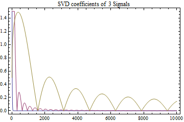

In Figure 1 (left) we see the SVD representation of three signals: a very smooth signal , a smooth signal and a rough signal , the attributes coming from the interpretation via the decay of Fourier coefficients. The weakly balanced oracle indices are . So, we stop before in the super-smooth case and expect a high variability of around . The strong indices are . For the smooth and super-smooth case with rapid decay and oscillations the signals lie in the class from (4.2) for relatively small only, which explains why here occurs.
We choose although the ratio , defining the constant , is about at . The relationship (3.1) therefore indicates that a smaller value of might be beneficial, which indeed in practice yields much better results, especially for the smooth and rough cases. In any case, in this simulation we use off the shelf and we compute the stopping rule starting at to illustrate the effects when very early stopping is recommended.
For the smooth signal Figure 1 (right) displays squared bias, variance and residuals (for one realisation) as a function of the number of iterations and indicates the stopping indices (the bias and variance functions are rescaled to fit into the picture). We see that the residual and its expected value are hardly distinguishable and thus is very close to the oracle proxy . While our error analysis uses the weak norm oracle inequality to establish the strong norm bound, here the strongly balanced oracle is closer to than the weak counterpart . The effects will become obvious in the error plots below.
Relative to the target , Figure 2 (left) displays box plots (a box representing the inner quartile range, whiskers the main support, points outliers and a horizontal bar the mean) for the relative number of iterations and , respectively, in 1000 Monte Carlo repetitions and for the three signals. We see the high variability for the super-smooth signal and the fact that for all three signals usually stops too early. For the weak norm this can be cured by choosing smaller taking into account the size of , as discussed above (independently of the unknown signal). Relative to the strongly balanced oracle , however, the stopping rule comes closer to the oracle for the super-smooth and smooth signals and moves further away for the rough signal because of and , respectively.


In Figure 2 (right) the box plots show for the same Monte Carlo run the relative errors (weak norm) and (strong norm) such that higher values indicate better performance. As expected from the stopping rule results, the variability is largest for the super-smooth case, and as predicted by theory, the relative efficiency in weak norm is best for the rough signal. In strong norm all three efficiencies become much better. Due to this was to be expected for the super-smooth and smooth signals, cf. also Figure 1 (right). For the rough signal this is quite surprising because the stopping rule usually stops at about half the value of . This is explained by a roughly linear decay of around and a strong growth in such that the total error is quite flat to the left of . Note that in weak norm decays much faster and the ’flatness’ disappears. This is the common phenomenon that the relative error due to a data-driven parameter choice often becomes smaller for ill-posed than for well-posed settings.
Further unreported simulations confirm these findings, in particular the relative error due to residual-based stopping remains small (rarely larger than , i.e. relative efficiency usually larger than ). Only for super-smooth signals, where we ought to stop before , the variability may become harmful.
As a practical procedure, we propose to run the iterations always until (51 iterates here) and if the stopping rule tells us not to continue, then we apply a standard model selection procedure to choose among the first iterates. For the truncated SVD case this two-step procedure can be proven to be rate-optimal for all regularities , not only within the adaptation interval, see [6]. For our general spectral regularisation approach the lack of a complete oracle inequality in strong norm is due to potentially stopping later than at . Hence, a natural suggestion would be to apply a second model selection step to select among for any outcome of . The performance of this general two-step approach needs to be studied further, but seems very promising from the perspective of both, statistical errors and numerical complexity.
5 Appendix
5.1 Proof of Proposition 2.6
We start with an important result for a nonincreasing sequence satisfying (S). This is related to comparisons between a function and its power integrals, also known as Karamata’s one-sided relations.
5.1 Lemma (One-sided Karamata relations).
Suppose Assumption (S) is satisfied. Then for any and we have
| for and , | (5.1) | |||||
| for and , | (5.2) | |||||
| for and . | (5.3) |
Proof.
We will need the following auxiliary result:
5.2 Lemma.
Suppose Assumptions (S) and (R) are satisfied with , then the constant defined via (2.4) is such that
| (5.4) |
It follows, for any :
| (5.5) |
Proof.
Proof of Proposition 2.6.
The monotonicity, continuity and limiting behaviour of in for fixed required from R1 ensure the basic requirements on the filter sequence (namely continuous, and as ). Since the spectral sequence is nonincreasing, the monotonicity in of ensures the validity of A2. Similarly, Assumption R2 transparently ensures A1.
We turn to checking A4. For this we use (5.1) with , yielding
We now check A5 for . Denote , where is from (5.4). Introduce . Property and (5.4) imply . Assumption R3 and (2.5) ensure for all , so that
| (5.6) |
To control the second term (present only if ), we note that, since , (5.3) yields
We apply this relation to . We deduce from and
We finally turn to A3. Without loss of generality we can assume in (R3). As for all
| (5.7) |
it follows that condition (R3) implies for all :
| (5.8) |
Denote ; the above implies together with (2.5) that . We infer that for :
while
The desired bound A3 with for some constant follows from . It therefore suffices to establish for all :
| (5.9) |
i.e., to check the inequality
Using (5.7) again, it is sufficient to check the above inequality when replacing everywhere by , and by .
Denoting , we thus have to establish the sufficient condition (for some constant )
| (5.10) |
Writing the left fraction as and the right fraction (without ) as , we check this relation by bounding for , . Without loss of generality we assume (otherwise some products are just zero). Let us recall that (5.1) implies that
| (5.11) |
for . We will also need below a similar bound with replaced by on the left-hand side. For this, notice that by Assumption (S) we have , combining with (5.11) we get:
| (5.12) |
with . The first term to handle is now (using (5.11)):
For the second term we clearly have . The third term (using (5.12) and the definition of ) is bounded as:
For the fourth term we bound, using the definition of ,
Hence, (5.10) is established if we choose . ∎
5.2 Proof of Lemma 2.7
We start with considering the case . Let us introduce the spectral distribution function for . Then Assumption (S) gives for :
so that taking in the above display yields , provided . We will apply the relation for below, and check
Set again . Under Assumption (R) we conclude for
This establishes the first inequality. In the other direction, denote, as in the proof of Prop. 2.6, , where with from (5.4). Under Assumption R3 we have
We concentrate on the second term and assume without loss of generality that (otherwise this term vanishes). If , we use the Karamata relations (5.3), then (5.2), and , to bound
If , then directly using (2.8) and :
which implies that the inequality derived in the first case still holds. Additionally, since from Lemma 5.2 and , we have , so that
Altogether, we obtain the second inequality:
We turn to the case . Then Assumption R3 implies that for all we have . It follows from this and (5.1):
establishing the first bound in this case. The inequality in the other direction follows directly from
5.3 Maximal inequality for weighted -variables with drift
We first recall a result on the concentration of weighted chi-squared type random variables.
5.3 Lemma (Laurent and Massart, Lemma 1 in [19]).
Let be i.i.d. variables. For nonnegative numbers set
With the following inequalities hold for any :
| (5.13) | ||||
| (5.14) |
and also
Lemma 5.3 is stated in a slightly more general setting, since the original result of Laurent and Massart [19], based itself on Lemma 8 in Birgé and Massart [4], has no maximum in for the definition of . The proof, however, is based on the classical Chernov bound argument, which readily carries over with a maximum: indeed, for and ,
by Doob’s maximal inequality applied to the submartingale .
5.4 Lemma.
References
- [1] A.B. Bakushinskii. Remarks on the choice of regularization parameter from quasioptimality and relation tests. Zh. Vychisl. Mat. i Mat. Fiz. (Russian), 8:1258–1259, 1984.
- [2] F. Bauer and M. Reiß. Regularization independent of the noise level: an analysis of quasi-optimality. Inverse Problems, 24(5):055009, 2008.
- [3] N. H. Bingham, C. M. Goldie, and J. L. Teugels. Regular Variation. Cambridge University Press, 1989.
- [4] L. Birgé and P. Massart. Minimum contrast estimators on sieves: exponential bounds and rates of convergence. Bernoulli, 4(3):329–375, 1998.
- [5] N. Bissantz, T. Hohage, A. Munk, and F. Ruymgaart. Convergence rates of general regularization methods for statistical inverse problems and applications. SIAM Journal on Numerical Analysis, 45:2610–2636, 2007.
- [6] G. Blanchard, M. Hoffmann, and M. Reiß. Early stopping for statistical inverse problems via truncated SVD estimation. Technical report, arXiv: 1710.07278, 2017.
- [7] G. Blanchard and P. Mathé. Discrepancy principle for statistical inverse problems with application to conjugate gradient iteration. Inverse Problems, 28:pp. 115011, 2012.
- [8] L. Brown and M. Low. Asymptotic equivalence of nonparametric regression and white noise. Annals of Statistics, 24:2384–2398, 1996.
- [9] L. Cavalier. Inverse problems in statistics. In Inverse problems and high-dimensional estimation, pages 3–96. Lecture Notes in Statistics 203, Springer, 2011.
- [10] L. Cavalier and Y. Golubev. Risk hull method and regularization by projections of ill-posed inverse problems. Annals of Statistics, 34:1653–1677, 2006.
- [11] A. Cohen, M. Hoffmann, and M. Reiß. Adaptive wavelet Galerkin methods for linear inverse problems. SIAM Journal on Numerical Analysis, 42(4):1479–1501, 2004.
- [12] D. Djurcić, R. Nikolića, and A. Torgasev. The weak asymptotic equivalence and the generalized inverse. Lithuanian Mathematical Journal, 50(1):34–42, 2010.
- [13] H. Engl, M. Hanke, and A. Neubauer. Regularization of Inverse Problems. Kluwer Academic Publishers, London, 1996.
- [14] A. Fleige. Characterizations of monotone -regularly varying functions by means of indefinite eigenvalue problems and help type inequalities. Journal of Mathematical Analysis and Applications, 412:1479–1501, 2014.
- [15] Y. Golubev. Adaptive spectral regularizations of high dimensional linear models. Electronic Journal of Statistics, 5:1588–1617, 2011.
- [16] P. C. Hansen. Discrete inverse problems: insight and algorithms, Fundamentals of Algorithms 7. SIAM, 2010.
- [17] I. Karatzas and S.E. Schreve. Brownian motion and stochastic calculus. Springer Berlin Heidelberg, 2nd edition, 1991.
- [18] S. Kindermann. Discretization independent convergence rates for noise level-free parameter choice rules for the regularization of ill-conditioned problems. Electronic Transactions on Numerical Analysis, 40:58–81, 2013.
- [19] B. Laurent and P. Massart. Adaptive estimation of a quadratic functional by model selection. The Annals of Statistics, 28:1302–1338, 2000.
- [20] S. Lu and P. Mathé. Discrepancy based model selection in statistical inverse problems. Journal of Complexity, 30:386–407, 2014.
- [21] B. Mair and F.H. Ruymgaart. Statistical estimation in Hilbert scale. SIAM Journal on Applied Mathematics, 56:1424–1444, 1996.
- [22] P. Mathé and S. V. Pereverzev. Geometry of linear ill-posed problems in variable Hilbert scales. Inverse problems, 19(3):789, 2003.
- [23] S. Pereverzev and E. Schock. On the adaptive selection of the parameter in regularization of ill-posed problems. SIAM Journal on Numerical Analysis, 43:2060–2076, 2005.
- [24] M. Reiß. Asymptotic equivalence for nonparametric regression with multivariate and random design. Annals of Statistics, 36(4):1957–1982, 2008.
- [25] G. Wahba. Practical approximate solutions to linear operator equations when the data are noisy. SIAM Journal on Numerical Analysis, 14(4):651–667, 1977.