Solar Neutrino Measurements in Super–Kamiokande–IV
Abstract
Upgraded electronics, improved water system dynamics, better calibration and analysis techniques allowed Super-Kamiokande-IV to clearly observe very low-energy 8B solar neutrino interactions, with recoil electron kinetic energies as low as 3.49 MeV. Super-Kamiokande-IV data-taking began in September of 2008; this paper includes data until February 2014, a total livetime of 1664 days. The measured solar neutrino flux is assuming no oscillations. The observed recoil electron energy spectrum is consistent with no distortions due to neutrino oscillations. An extended maximum likelihood fit to the amplitude of the expected solar zenith angle variation of the neutrino-electron elastic scattering rate in SK-IV results in a day/night asymmetry of . The SK-IV solar neutrino data determine the solar mixing angle as , all SK solar data (SK-I, SK-II, SK III and SK-IV) measures this angle to be , the determined mass-squared splitting is eV2.
pacs
14.60.PqI Introduction
Solar neutrino flux measurements from Super-Kamiokande (SK) [1] and the Sudbury Neutrino Observatory (SNO) [2] have provided clear evidence for solar neutrino flavor conversion in which electron flavor neutrinos convert to either muon or tau flavor neutrinos. This flavor conversion is well described by flavor oscillations of three neutrinos. In particular, the extracted oscillation parameters agree with nuclear reactor anti-neutrino measurements [3]. However, while oscillations of reactor antineutrinos at the solar frequency were observed, there is still no clear evidence that the solar neutrino flavor conversion is indeed due to neutrino oscillations and not caused by another mechanism. Currently there are two types of testable signatures unique to neutrino oscillations, the first being the observation and precision test of the Mikheyev–Smirnov–Wolfenstein (MSW) resonance curve [4], the characteristic energy dependence of the flavor conversion (assuming oscillation parameters extracted from solar neutrino and reactor anti-neutrino measurements): higher energy solar neutrinos (higher energy 8B and neutrinos) undergo adiabatic resonant conversion within the Sun (present data imply a survival probability of about ), while the flavor changes of the lower energy solar neutrinos (, 7Be, , CNO and lower energy 8B neutrinos) arise only from vacuum oscillations. These averaged vacuum oscillations lead to an average survival probability which – for sufficiently small mixing – must exceed (present data imply about ). The transition from the matter-dominated oscillations within the Sun to the vacuum-dominated oscillations should occur near three MeV. This makes 8B neutrinos the best choice when looking for a transition point within the energy spectrum. A second signature unique to oscillations arises from the effect of the terrestrial matter density on solar neutrino oscillations. This effect is tested directly by comparing solar neutrinos that pass long distances through the Earth at nighttime to those which do not pass through the Earth during the daytime. Those neutrinos which pass through the Earth will generally have an enhanced electron neutrino content, leading to an increase in the nighttime electron elastic scattering rate (or any charged-current interaction rate), and hence a negative “day/night asymmetry” , where () is the daytime (nighttime) rate and is the average rate. SK is sensitive to 8B and hep solar neutrinos in the energy range around 4 to MeV and precisely measures the neutrino interaction time. It is therefore a good detector to search for both solar neutrino oscillation signatures.
SK [5] is a large, cylindrical, water Cherenkov detector containing of 50,000 tons of ultra-pure water. It is located 1,000 m beneath the peak of Mount Ikenoyama, in Kamioka Town, Japan. The SK detector is optically separated into a 32.5 kton cylindrical inner detector (ID) surrounded by a meter water shield, m of which is the active veto outer detector (OD). The structure dividing the detector regions contains an array of photo-multiplier tubes (PMTs). SK started data-taking in April of 1996, with 11,146 ID and 1,885 OD PMTs, and was then shut down for maintenance in June of 2001. This period is called SK-I [1]. While refilling the tank with water in November of 2001, a PMT implosion caused a chain reaction which destroyed of the PMTs. The surviving and new PMTs were redistributed and covered with fiber-reinforced plastic (FRP) and acrylic cases, in order to avoid another accidental chain reaction. Data-taking re-started with 5,182 ID and 1,885 OD PMTs in December of 2002, and the period until October of 2005 is called SK-II [6]. In October of 2006, newly manufactured PMTs replaced those which had been destroyed, and with 11,129 ID and 1,885 OD PMTs data-taking resumed as the SK-III phase [7]. The fourth phase of SK (SK-IV) began in September of 2008, with new front-end electronics (QTC Based Electronics with Ethernet, QBEE [8]) for both the ID and OD, new data acquisition system, and continues to this day. This paper will include data taken up until the beginning of February 2014.
Improvements in the front-end electronics, the water circulation system, calibration techniques and the analysis methods have allowed the SK-IV solar neutrino measurements to be made with a lower energy threshold and smaller systematic uncertainties, compared to SK-I, II and III. The hardware and software improvements are summarized in section II, while the SK-IV data set, data reduction, and its systematic uncertainty estimations on the total flux are detailed in section III. The simulation of solar neutrino events in SK is described also in section III. Unfortunately, the simulation code for the SK-III period used in [7] was inaccurate, which affected the input recoil electron spectrum. The details (and the correction applied) as well as a reanalysis of the SK-III data are briefly described in section III and Appendix A.
In section IV, the energy spectrum results of SK-IV as well as all SK phases combined are discussed. Section V presents the SK-IV day/night asymmetry analysis. Finally, section VI contains an oscillation analysis of SK-IV data by themselves and in combination with other SK phases, and also a global analysis which combines the SK results with other relevant experiments.
II Detector Performance
II.1 Electronics, Data acquisition system
To ensure stable observation and to improve the sensitivity of the detector, new front-end electronics called QBEEs were installed, allowing for the development of a new online data acquisition system. The essential components on the QBEEs used for the analog signal processing and digitization are the QTC (high-speed Charge-to-Time Converter) ASICs [8], which achieve very high speed signal processing and allow the integration of the charge and recording of the time of every PMT signal. These PMT signal times and charge integrals are sent to online computers, where a software trigger searches for timing coincidences within 200 ns to pick out events in a similar fashion as the hardware “hitsum trigger” did in SK-I through III [1, 6, 7]. The energy threshold of this coincidence trigger is determined by the number of coincident PMT signals that are required: a smaller coincidence level will be more sensitive to lower energy events, but will result in larger event rates. The definitions of the different trigger types and the corresponding typical event rates are summarized in Table 1. Since all PMT signals are digitized and recorded, there is no deadtime of the detector from a large trigger rate, so the efficiency of triggering on HE events does not limit the maximum possible rate of SLE triggers; only the processing capability of the online computers limits this maximum rate. The software trigger system uses flexible event time periods (1.3 sec for SLE, 40 sec for LE and HE). The trigger efficiencies for the thresholds are () between 3.49 and 3.99 MeV (3.99 and 4.49 MeV) and above 4.49 MeV.
| Trigger Type | Hits in 200 ns | Trigger Rate |
|---|---|---|
| Super Low Energy (SLE) | 34 | 3.0-3.4 kHz |
| Low Energy (LE) | 47 | Hz |
| High Energy (HE) | 50 | Hz |
II.2 Water system
To keep the long light attenuation length of the SK water stable, the water is continuously purified with a flow rate of 60 ton/hour. Purified water supplied to the bottom of the detector replaces water drained from its top. A higher temperature of the supply water than the detector temperature results in convection throughout the detector volume. This convection transports radioactive radon gas, which is produced by radioactive decays from the U/Th chain near the edge of the detector into the central region of the detector. Radioactivity coming from the decay products of radon gas (most commonly 214Bi beta decays) mimics the lowest energy solar neutrino events. In January of 2010, a new automated temperature control system was installed, allowing for control of the supply water temperature at the degree level. By controlling the water flow rate and the supply water temperature with such high precision, convection within the tank is kept to a minimum and the background level in the central region has since become significantly lower.


II.3 Event reconstruction
The methods used for the vertex, direction, and energy reconstructions are the same as those used for SK-III [7]. The Cartesian coordinate system for the SK detector is shown in Fig. 1.
II.3.1 Vertex
The vertex reconstruction is a maximum likelihood fit to the arrival times of the Cherenkov light at the PMTs [6]. Fig. 2 shows the vertex resolution for each SK phase. The large improvement in SK-III compared to SK-I is the result of using an advanced vertex reconstruction program, while the improved timing resolution and slightly better agreement of the timing residuals between data and Monte Carlo (MC) simulated events are responsible for the additional improvement of SK-IV. We observed a bias in the reconstructed vertex called the vertex shift. This vertex shift is measured with a gamma-ray source at several positions within the SK detector: neutrons from spontaneous fission of 252Cf are thermalized in water and then captured on nickel in a spherical vessel [5, 11]. The nickel then emits 9 MeV gammas (Ni calibration source). Fig. 3 shows the shift of the reconstructed vertex of these Ni gammas in SK-IV from their true position (assumed to be the source position). The SK-IV vertex shift is improved compared with SK-I, II and III [5, 6, 7].

II.3.2 Direction
A maximum likelihood fit comparing the Cherenkov ring pattern of data to MC simulations is used to reconstruct event directions. During the SK-III phase an energy dependence was included in the likelihood and the angular resolution was improved by about (10 MeV electrons) compared to SK-I. The angular resolution in SK-IV is similar to that in SK-III.
II.3.3 Energy
The energy reconstruction is based on the number of PMT hits within a 50 ns time window, after the photon travel time from the vertex is subtracted. This number is then corrected for water transparency, dark noise, late arrival light (due to scattering and reflection), multi-photon hits, etc., producing an effective number of hits (see [7]). Simulations of mono-energetic electrons are used to produce a function relating to the recoil electron energy (MeV).
The water transparency parameter used in the energy reconstruction is measured using decay electrons from cosmic-ray muons. This method of obtaining the water transparency is the same as for SK-I, II and III [1, 6, 7]: exploiting the azimuthal symmetry of the Cherenkov cone, we determine the light intensity as a function of light travel distance and fit it with an exponential light attenuation function. The top panel of Fig. 4 shows the time variation of the measured water transparency, while the bottom panel shows the reconstructed mean energy of decay electrons in black (red) before (after) water transparency corrections have been applied. The stability of the water transparency corrected energy reconstruction is within (dashed lines).


II.3.4 Multiple scattering goodness (MSG)
Even at the low energies of the recoil electrons from 8B solar neutrino-electron scattering, the PMT hit pattern from the Cherenkov cone reflects the amount of multiple Coulomb scattering recoil electrons experience. Very low-energy electrons will incur such scattering more than higher energy electrons and thus have a more isotropic PMT hit pattern. Radioactive background events, such as 214Bi beta decays, generally have less energy than 8B recoil electrons. Radioactive background events with emission will be more isotropic still. The “goodness” of a directional fit characterizes this hit pattern anisotropy: it is constructed by first projecting cones from the vertex position, centered around each PMT that was hit within a 20 ns time window (after time of flight subtraction). Pairs of such cones are then used to define “event direction candidates”, which are vectors along the intersection lines of the two cones. Only cone pairs which intersect twice are used to define event direction candidates. Fig. 5 shows a schematic view of how the event direction candidates are found. The yellow points represent hit PMTs, which will roughly be found around the Cherenkov “ring”, the projection of the cone onto the inner detector wall shown by the gray circle. As seen in the figure, for pairs of PMTs with positions located near the Cherenkov ring, one of the intersection lines shown by the black crosses will fall close to the best fit direction vector shown as the black point on the inner detector wall which this vector passes through. Clusters of these event direction candidates are then found by associating other event direction candidates which are within of a “central event direction” seeded by the candidates themselves. Once an event direction candidate has been associated to a cluster, it then will not seed another cluster. The event direction candidate vectors of a cluster are added together to adjust the central event direction. Several iterations of this adjustment with subsequent cluster reassignment will center the clusters and maximize the magnitude of the vector sum. The vector sum with the largest magnitude is kept as the “goodness direction”. The multiple scattering goodness (MSG) is then defined by the ratio of this magnitude and the number of event direction candidates within the 20 ns time window. The filled squares (error bars) and solid (dotted) lines of Fig. 6 compare the LINAC data and MC MSG distributions for 4.38 MeV (8.16 MeV) electrons. As expected, higher energy electrons have a larger mean MSG.


II.4 Energy calibration
The absolute energy scale is determined by an electron linear accelerator (LINAC) [9]. The LINAC calibration system injects single monoenergetic electrons into SK in the downward direction. The energy of the momentum-selected electrons is precisely measured by a germanium (Ge) detector using a thin titanium window similar to that used under the water. To determine the energy scale, 6.28 and 12.93 MeV electron data are compared to simulated events. Fig. 7 shows the dependence of this comparison. We cross-check the energy scale obtained from the LINAC energy with 16N / decays, which originate from the (n,p) reaction of 16O with neutrons produced by a deuterium-tritium (DT) fusion neutron generator [10]. The 10.5 MeV endpoint 16N decays of the DT calibration are isotropic, with of the decays emitting a 6 MeV in conjunction with an electron. DT-produced 16N data are taken at a much larger number of positions in SK than LINAC data. Fig. 8 compares the reconstructed energy of 16N simulated events with data, as a function of the position of the production. Fig. 9 shows the directional dependence of the energy scale, with respect to the detector zenith angle. The two bins between and 1 are affected by increased shadowing from the DT generator. Conservatively, we fit the entire data with a linear combination of a constant and an exponential function to estimate the systematic uncertainty on the day/night asymmetry due to the directional dependence of the bias of the reconstructed energy.
The systematic uncertainty of the energy scale due to position (direction) dependence is estimated to be (). The effect of the water transparency variation during LINAC calibration is estimated to be , while the uncertainty of the LINAC electron beam energy (as measured by the Ge detector), is estimated to be . The total systematic uncertainty of the absolute energy scale thus becomes , calculated by adding all the contributions in quadrature, and is summarized in Table 2. These uncertainties are similar to those in SK-III ().

| Position Dependence | |
|---|---|
| Direction Dependence | |
| Water Transparency | |
| LINAC Energy | |
| Total |
The detector’s energy resolution is determined using the same method as described in [7]. Monoenergetic electrons are simulated and used to determine the relationship between the effective number of hits in the detector and the electron energy in MeV. Using the width of Gaussian fits to the energy distributions resulting from these simulated electrons, the energy dependence of the energy resolution is well described by the function
| (1) |
in units of MeV, where is electron total energy. This is comparable to the SK-III energy resolution, given as in [7].
II.5 Light propagation in water
II.5.1 Water parameters
The water transparency in the MC simulation is determined using absorption and scattering coefficients as a function of wavelength (full details of this and other more general detector calibrations can be found in [11]). These coefficients are independently measured by a nitrogen laser and laser diodes at five different wavelengths: 337 nm, 375 nm, 405 nm, 445 nm and 473 nm. Based on these measurements, the dominant contribution to the variation of the water transparency is a variation in the absorption length. The absorption coefficient is time and position dependent, as explained below. This SK-IV solar neutrino analysis only varies the absorption, and uses a single set of time independent scattering coefficients, as measured by the laser diodes [11].
II.5.2 Time dependence
To track the absorption time dependence, we measure the light attenuation of Cherenkov light from decay electrons (from cosmic-ray muons stopping throughout the SK inner detector volume). This measurement uses the azimuthal symmetry of the emitted Cherenkov cone to compare different light propagation path lengths within the same event and assumes a simple exponential attenuation. This effective attenuation length is one of the energy reconstruction parameters. The top panel of Fig 4 shows the decay electron water transparency parameter as a function of time.
In orer to connect the absorption time dependence in the MC to the water transparency parameter measured by decay electrons we generate mono-energetic electron samples throughout the detector for a wide range of absorption coefficients with nine different energies between 4 and 50 MeV. Each MC sample is assigned a particular decay electron water transparency parameter that minimizes the difference between input energy and average reconstructed energy. As expected, the relationship between water transparency and MC absorption coefficent does not significantly depend on the generated energy. The same procedure establishes the relationship between the (corrected) number of PMT hits and energy. Fig. 10 shows the obtained relationship between absorption coefficient and water transparency parameter. For convenience we measure the absorption coefficient relative to the coefficient at the time of the LINAC calibration data-taking, which defines the energy scale (see [11]). We employ a linear interpolation between the data points. The mean energy of these decay electrons is used to evaluate the systematic uncertainty of the time dependence of the energy scale (see bottom panel of Fig. 4). After correction for the time variation of the absorption coefficient, the apparent time dependence of the decay electron mean energy becomes smaller than .


II.5.3 Position dependence
As already explained, the water in the SK detector is continuously recirculated through the SK water purification system. Water is drained from the detector top, purified, and re-injected at the bottom. Due to careful temperature control of the injected water, the convection inside the SK tank is suppressed everywhere but at the bottom part of the tank below m. Fig. 11 shows the typical water temperature as a function of in the SK detector. The temperature is uniform below m, where convection is occurring and increases steadily above that. We assume that absorption is strongly correlated with the amount of convection and model the position dependence of the absorption length as constant below m and linearly changing above m:
where parametrizes the -dependence of the absorption. The parameter is determined by studying the distribution of hit PMTs of Ni calibration data (see section II.3) [11] in the “top”, “bottom” and “barrel” regions of the detector (see Fig. 1). After other detector asymmetries like quantum efficiency variations of the PMTs are taken into account, the hit rate of the top region in the detector is lower than that of the bottom region. is then fit using the hit asymmetry of Ni calibration events. Since the Ni calibration hit pattern varies with time, both and depend on time. The Xe flash lamp scintillator ball calibration system [11] tracks the time dependence: a Xe flash lamp powers a scintillator ball located near the middle of the detector. The time dependence of is also monitored by Ni calibration data. The introduction of into the MC simulation has helped to reduce the systematic uncertainty on the energy scale, as it addresses a significant contribution to its directional dependence. This is important for the solar neutrino day/night asymmetry analysis.
III Data Analysis
After installation of the new front-end electronics, SK-IV physics data-taking started on October 6, 2008. This paper includes data taken from October 6, 2008 until February 1, 2014. The total livetime is 1664 days. The entire data period was taken with a new very low energy threshold of 34 hits within ns (cf. Table 1). To reduce the required data storage capacity, obvious backgrounds are removed using faster and less-stringent implementations of the analysis cuts on fiducial volume, energy, ambient events and external events, before the data is permanently stored. By applying these pre-cuts, the data load was reduced to of its original size.
III.1 Event selection
Most of the cuts used are the same as those used in SK-III [7], but some of the cut values and the energy regions in which they are applied are changed to optimize the significance: if () is the number of signal (background) events, we define the significance as . Also, as was the case in SK-III, below 4.99 MeV the fiducial volume is reduced since backgrounds appear localized at the bottom of the detector and at large radii.
III.1.1 Ambient background reduction
As in [1, 6, 7], several cuts remove low-energy radioactive backgrounds. These backgrounds originate mostly from the PMT enclosures, the PMT glass, and the detector wall structure. While the true vertices lie outside the fiducial volume, some radioactive background events are mis-reconstructed inside the fiducial volume. The quality of the event reconstruction is tested by variables describing its goodness. The first variable is a timing goodness testing the “narrowness” of the PMT hit timing residuals, which is defined in [6] (section III.B, equation 3.1). The second is a hit pattern goodness testing the azimuthal symmetry of the Cherenkov cone ( is perfectly symmetric, is completely asymmetric). Good single electron events must have greater than 0.2. Events below 6.99 MeV (4.99 MeV) must have greater than 0.25 (0.29). The same cut was applied for SK-III.

We also check the consistency of the observed light pattern with a single Cherenkov cone as in [1] (section VII.C, equation 7.4). This cut will remove events with multiple Cherenkov cones, e.g., from beta decays to an excited nuclear state with subsequent gamma emission. The hit pattern is assigned a likelihood based on the direction fit likelihood function. Fig 12 shows the likelihood and cut criteria in three different energy ranges. Further details are found in [12].
A small hit cluster cut targets radioactive background events in the PMT enclosures or glass, which coincide with an upward fluctuation of the PMT dark noise. Only events with a reconstructed bigger than 155 m2 (120 m2), a reconstructed smaller than m ( m), or a reconstructed bigger than 13 m, for reconstructed energies in MeV ( MeV), are subject to this cut. To characterize small hit clusters, we select PMT hits with times coincident within 20 ns (after time-of-flight subtraction, see section II.3.3), and then find the smallest sphere around any of the selected PMTs that encloses at least of all selected PMTs. This radius is multiplied by the ratio of PMT hits coincident within 20 ns (without time-of-flight correction) divided by (see section II.3.3). Solar neutrinos near the edge of the fiducial volume have a bigger radiushit ratio (see also section III C in [7], Fig. 17 and 18) than the radioactive background. As in SK-III, we remove events with radiushit ratio less than 75 cm as shown in Fig. 12.
Source (cm) (cm) (cm) Xenon flasher 353.5 0.0 LED 35.5 150.0 TQ Diffuser Ball 100.0 DAQ Rate Test Source 353.5 100.0 Water Temp. Sensors 1 1200 Water Temp. Sensors 2 70.7
Finally, we remove spurious events due to various calibration sources (mostly radioactiv decays), if they are below 4.99 MeV. A reconstructed position closer than 2 m to the source, or closer than 1 m to the source or water temperature sensor cable (all cables run along the axis from the top down to the source position) means the event is removed. Table 3 lists the various calibration sources which are considered. The fiducial volume is reduced by about 0.48kton due to this cut.
III.1.2 External event cut
To remove radioactive background coming from the PMTs or the detector wall structure, we calculate the distance to the PMT-bearing surface from the reconstructed vertex looking back along the reconstructed event direction. Radioactive backgrounds tend to appear “incoming”, so we remove events where this distance is small. Solar neutrino candidates above 7.49 MeV (above 4.99 MeV and below 7.49 MeV) must have a distance of at least 4 m (6.5 m). In the energy region below 4.99 MeV we distinguish between the “top” (cylinder top lid), “barrel” (cylinder side walls) and “bottom” (cylinder bottom lid) surfaces, shown in Fig. 1. Candidates which come from the “top” (“bottom”) must have a distance of at least 10 m (13 m), while “barrel” event candidate distances must exceed 12 m. SK-III applied the same cuts.
III.1.3 Spallation cut
Some cosmic-ray ’s produce radioactive elements by breaking up an oxygen nucleus [13]. A spallation event occurs when these radioactive nuclei eventually decay and emit ’s and/or ’s. A spallation likelihood function is made from the distance of closest approach between the preceding track(s) and a solar neutrino candidate, their time difference, and the charge deposited by the preceding (s). By using the likelihood function spallation-like events are rejected, see [1, 14] for details.
When lower energy cosmic-ray ’s are captured by 16O nuclei in the detector, 16N can be produced which decays with gamma-rays and/or electrons with a half-life of 7.13 seconds. In order to reject these events, the correlation between stopping ’s in the detector and the remaining candidate events are checked. The cut criteria for 16N events is as follows; (1) reconstructed vertex is within 250 cm to the stopping point of the , (2) the time difference is between 100 sec and 30 sec.
To measure their impact on the signal efficiency, the spallation and 16N cuts are applied to events that cannot be correlated with cosmic-ray muons (e.g. candidates preceding muons instead of muons preceding candidates). This “random sample” then measures the accidental coincidences rate between the muons and subsequent candidate events. The spallation (16N) cut reduces signal efficiency by about 20 (0.53).
III.1.4 Fiducial volume cut
Events which occur near the wall of the detector (reconstructed within 2 m from the ID edge) are rejected. The volume of this fiducial volume is 22.5 kton. Below 4.99 MeV this cut is tightened. Fig. 13 shows the vs. data vertex distribution for 3.49 to 3.99 MeV, after the above cuts. Each bin shows the rate (events/day/bin), with blue showing a lower rate and red a higher rate. We expect solar neutrino events to be uniformly distributed throughout the detector volume, and the regions with high event rates are likely dominated by background. To increase the significance in the final data sample for this energy region (3.49 to 4.49 MeV), we have reduced the fiducial volume to the region shown by the black line in the figure and described by
| (4) |
where the coordinates are given in meters. This function was chosen in order to approximately follow the contours of constant event rate. For the energy range of 4.49 to 4.99 MeV, events which have or m are cut.

III.1.5 Other cuts
Short runs ( minutes), runs with hardware and/or software problems, and calibration runs are not used for this analysis. Cosmic-ray events are removed by rejecting events with more than 400 hit PMTs, which corresponds to about 60 MeV for electron type events.
III.1.6 Summary
Fig. 14 shows the energy spectrum after each reduction step and Fig. 15 shows the reduction efficiency of the corresponding steps. The final sample of SK-IV data is shown by the filled squares and for comparison the SK-III final sample is superimposed (dashed lines). Above 5.99 MeV, the efficiency for solar neutrinos in the final sample is almost the same as in SK-III, while for 4.99 to 5.99 MeV, the SK-IV efficiency is better than SK-III. The reason for the improvement is the removal of a fiducial volume cut based on the “second vertex fit” [7, 1] and making a looser ambient event cut. The reduced fiducial volume and a tighter ambient event cut for 3.49 to 4.99 MeV results in a lower efficiency than SK-III, but in exchange the background level has been reduced by .


III.2 Simulation of solar neutrinos
There are several steps in simulating solar neutrino events at SK: generate the solar neutrino fluxes and cross-sections, determine the recoil electron kinematics, track the Cherenkov light in water and simulate the response of the PMTs and electronics. We used the 8B solar neutrino spectrum calculated by Winter et al [15] and the solar neutrino spectrum from Bahcall et al [16]. The systematic uncertainties from these flux calculations are incorporated in the energy-correlated systematic uncertainty of the recoil electron spectrum. The simulated event times are chosen according to the livetime distribution of SK-IV so that the solar zenith angle distribution of the solar neutrinos is reflected correctly across the simulated events. The recoil electron energy spectrum is calculated by integrating the differential cross section between zero and . is the maximum kinetic energy of the recoiling electron, which is limited by the incident neutrino energy.
Because ’s scatter via both and exchange, while ’s interact only in the neutral-current channel, the , cross section is approximately six times larger than ,. For the total and differential cross sections of those interactions, we adopted the calculation from [17], in which the radiative corrections are taken into account and where the ratio and depends on the recoil electron energy . Fig. 16 shows the differential cross section of , (solid) and (dashed) elastic scattering, for the case of 10 MeV incident neutrino energy. This recoil electron energy dependence of the cross section was accidentally omitted in the SK-III flux calculation in [7]. Therefore, wrong recoil electron kinematics were generated for the SK-III analysis, primarily affecting the lowest energy. We re-analyzed SK-III with the correct energy dependence (leaving everything else unchanged), the results of which can be found in Appendix A.
III.3 Total flux
In the case of interactions of solar neutrinos in SK, the incident neutrino and recoil electron directions are highly correlated. Fig. 17 shows the distribution for events in the energy range 3.49 to 19.5 MeV, as well as the definition of . In order to obtain the number of solar neutrino interactions, an extended maximum likelihood fit is used. This method is also used in the SK-I [1], II [6], and III [7] analyses. The likelihood function is defined as
| (5) |
where is the number of energy bins. The flux analysis of SK-IV has energy bins; 20 bins of 0.5 MeV width between 3.49 and 13.5 MeV, two energy bins of 1 MeV between 13.5 MeV and 15.5 MeV, and one bin between 15.5 MeV and 19.5 MeV. is the number of observed events in the -th energy bin. and , the free parameters of this likelihood function, are the number of solar neutrino interactions in all bins and the number of background events in the -th energy bin, respectively. is the fraction of signal events in the -th energy bin, calculated from solar neutrino simulated events. The background weights and the signal weights are calculated from the expected shapes of the background and solar neutrino signal, respectively (probability density functions). The background shapes are based on the zenith and azimuthal angular distributions of real data, while the signal shapes are obtained from the solar neutrino simulated events. The values of and are obtained by maximizing the likelihood. The histogram of Fig. 17 is the best fit to the data, the dark (light) shaded region is the solar neutrino signal (background) component of that best fit. The systematic uncertainty for this method of signal extraction is estimated to be .

III.3.1 Vertex shift systematic uncertainty
The systematic uncertainty resulting from the fiducial volume cut comes from event vertex shifts. To calculate the effect on the elastic scattering rate, the reconstructed vertex positions of solar neutrino MC events are artificially shifted following the arrows in Fig. 3, and the number of events passing the fiducial volume cut with and without the artificial shift are compared. Fig. 18 shows the energy dependence of the systematic uncertainty coming from the shifting of the vertices. The increase below 4.99 MeV comes from the reduced fiducial volume (smaller surface to volume ratio), not from an energy dependence of the vertex shift. The systematic uncertainty on the total rate is .

III.3.2 Trigger efficiency systematic uncertainty
The trigger efficiency depends on the vertex position, water transparency, number of hit PMTs, and response of the front-end electronics. The systematic uncertainty from the trigger efficiency is estimated by comparing Ni-calibration data (see section II.3) with MC simulation. For 3.49-3.99 MeV and 3.99-4.49 MeV, the difference between data and MC is and , respectively [12]. Above 4.49 MeV the trigger efficiency is and its uncertainty is negligible. The resulting total flux systematic uncertainty due to the trigger efficiency is .
III.3.3 Angular resolution systematic uncertainty
The angular resolution of electrons is defined as the angle which includes of events in the distribution of the angular difference between their reconstructed direction and their true direction. The MC prediction of the angular resolution is checked and the systematic uncertainty is estimated by comparing the difference in the reconstructed and true directions of LINAC data and LINAC (see [9]) simulated events. This difference is shown in Table 4 for various energies. To estimate the systematic uncertainty on the total flux, the signal shapes and are varied by shifting the reconstructed directions of the simulated solar neutrino events by the uncertainty in the angular resolution. These new signal shapes are used when extracting the total flux, and the resulting change in the extracted flux is taken as the systematic uncertainty from angular resolution.
| Energy (MeV) | SK-I() | SK-II() | SK-III() | SK-IV() |
|---|---|---|---|---|
| 4.0 | – | – | – | 0.64 |
| 4.4 | – | 0.74 | 0.68 | |
| 5.3 | – | – | – | |
| 6.3 | 2.32 | – | 0.02 | |
| 8.2 | 2.33 | 0.40 | 0.06 | |
| 10.3 | 1.52 | – | – | – |
| 12.9 | 1.07 | 0.22 | ||
| 15.6 | 0.88 | – | 0.39 | – |
| 18.2 | – | – | – | 0.31 |
SK-I SK-II SK-III SK-IV Threshold (MeV) 4.49 6.49 3.99 3.49 Trigger Efficiency Angular Resolution Reconstruction Goodness Hit Pattern Small Hit Cluster External Event Cut Vertex Shift Second Vertex Fit Background Shape Multiple Scattering Goodness Livetime Spallation Cut Signal Extraction Cross Section Subtotal Energy Scale Energy Resolution 8B Spectrum Total
III.3.4 Result
The systematic uncertainty on the total flux (between 3.49 and 19.5 MeV) is summarized in Table 5. The combined systematic uncertainty is calculated as the quadratic sum of all components, and found to be . This is the smallest systematic uncertainty of all phases of SK. In particular, the systematic uncertainties that are energy-correlated (arising from the energy scale and resolution uncertainty) are smallest: while SK-IV’s livetime is the same for all energy bins, previous phases have less livetime below 5.99 MeV recoil electron kinetic energy. For example, SK-III data below 5.99 MeV has only about half the livetime as the full SK-III phase. The improved livetime below 5.99 MeV, a higher efficiency in that energy region, and the additional data below 4.49 MeV all lessen the impact of energy scale and resolution uncertainties on the flux determination compared to previous phases. Other contributions to the reduction come from the removal of the fiducial volume cut based on an alternate vertex fit, and better control of vertex shift, trigger efficiency and angular resolution systematic effects. The number of solar neutrino events (3.49-19.5 MeV) extracted from Fig. 17 is (stat.)(syst.). This number corresponds to a 8B solar neutrino flux of
assuming a pure flavor content.
| Flux (/(cm2sec)) | |
|---|---|
| SK-I | |
| SK-II | |
| SK-III | |
| SK-IV | |
| Combined |
As seen in Table 6, the SK-IV measured flux agrees with that of previous phases within systematic uncertainty. It can then be combined with the previous three SK flux measurements to give the SK measured flux as
IV Energy Spectrum
Present values of and imply that solar neutrino flavor oscillations above about three MeV are dominated by the solar MSW [4] resonance, while low-energy solar neutrino flavor changes are mostly due to vacuum oscillations. Since the MSW effect rests solely on standard weak interactions, it is rather interesting to compare the expected resonance curve with data. Unfortunately multiple Coulomb scattering prevents the kinematic reconstruction of the neutrino energy in neutrino-electron elastic scattering interactions. However, the energy of the recoiling electron still provides a lower limit to the neutrino’s energy. Thus, the neutrino spectrum is inferred statistically from the recoil electron spectrum. Moreover, the differential cross section of ’s is not just a factor of about six smaller than the one for ’s, but also has a softer energy dependence. In this way, the observed recoil electron spectrum shape depends both on the flavor composition and the energy dependence of the composition of the solar neutrinos (see section III.2 in particular Fig. 16). Thus, even a flat composition of and would still distort the recoil electron spectrum compared to one with . The energy dependence of the day/night effect and rare neutrino interactions (with a higher endpoint than 8B ’s) also distort the spectrum.
Since the transition between MSW resonance and vacuum oscillations lies around 3 MeV, the lowest energy solar neutrinos show the largest deviation from the resonance electron survival probability. Here, we report for the first time, a clear solar neutrino signal with high statistics in the energy range 3.49-3.99 MeV observed over the entire data-taking period of SK-IV. Fig. 19 shows the solar angle distribution for this energy bin, with a distinct peak (above the background) coming from solar neutrinos. The number of solar neutrino interactions (measured in this energy range from fits to the distributions of Fig. 20 discussed below) is


IV.1 SK-IV spectrum results
As outlined in III.3 (in particular Eq. 5), the solar neutrino signal of SK-IV is extracted by an extended maximum likelihood fit. While the 8B flux analysis uses all 23 energy bins at once (and constrains the energy spectrum to the one expected from unoscillated simulation via the factors), we extract the solar neutrino energy spectrum by fitting one recoil electron energy bin at a time, with . Below 7.49 MeV, each energy bin is split into three sub-samples according to the MSG of the events, with boundaries set at MSG=0.35 and 0.45. These three sub-samples are then fit simultaneously to a single signal and three independent background components. The signal fraction in each MSG bin is determined by solar neutrino simulated events in the same manner as the factors in the 8B flux analysis. Similar to the 8B flux analysis, the signal and background shapes depend on the MSG bin : the signal shapes are calculated from solar neutrino simulated events and the background shapes are taken from data. Fig. 20 shows the measured angular distributions (as well as the fits) for the energy ranges 3.49-3.99 MeV, 3.99-4.49 MeV, 4.49-4.99 MeV and 6.99-7.49 MeV (from top to bottom), for each MSG bin (left to right). As expected in the lowest energy bins, where the dominant part of the background is due to very low-energy / decays, the background component is largest in the lowest MSG sub-sample. Also as expected, the solar neutrino elastic scattering peak sharpens as MSG is increased.
Using this method for recoil electron energy bins below 7.49 MeV gives improvement in the statistical uncertainty on the number of extracted signal events (the additional systematic uncertainty is small compared to the statistical gain). Fig. 21 shows the resulting SK-IV energy spectrum, where below 7.49 MeV MSG has been used and above 7.49 MeV the standard signal extraction method without MSG is used. Table C.1 gives the measured and expected rate in each energy bin, as well as that measured for the day and night times separately, along with the 1 statistical deviations. We re-analyzed the SK-III spectrum below 7.49 MeV with the same method, the same MSG bins and the same energy bins as SK-IV, down to 3.99 MeV. We also re-fit the entire SK-II (which has poorer resolution) spectrum using the same three MSG sub-samples. The gains in precision are similar to SK-IV. The SK-II and III spectra are given in section IV.3.

To analyze the spectrum, we simultaneously fit the SK-I, II, III and IV spectra to their predictions, while varying the 8B and neutrino fluxes within uncertainties. The 8B flux is constrained to /(cm2sec) and the flux to /(cm2sec) (motivated by SNO’s measurement [18] and limit [19]). The is described in detail in Section VI.
IV.2 Systematic uncertainties on the energy spectrum
| Energy (MeV) | 3.49-3.99 | 3.99-4.49 | 4.49-4.99 | 4.99-5.49 | 5.49-5.99 | 5.99-6.49 | 6.49-6.99 | 6.99-7.49 | 7.49-19.5 |
|---|---|---|---|---|---|---|---|---|---|
| Trigger Efficiency | - | - | - | - | - | - | - | ||
| Reconstruction Goodness | |||||||||
| Hit Pattern | - | - | - | - | - | ||||
| External Event Cut | |||||||||
| Vertex Shift | |||||||||
| Background Shape | |||||||||
| Signal Extraction | |||||||||
| Cross Section | |||||||||
| MSG | - | ||||||||
| Total |
Since we simultaneously fit multiple samples defined by the multiple Coulomb scattering goodness in the lowest recoil electron energy region, a systematic shift in this goodness of the data compared to solar 8B (or ) neutrino simulated events would affect the measured event rate in that energy region. To estimate the systematic effect of using MSG sub-samples, MSG distributions of LINAC data and simulated LINAC events were compared, as seen in Fig. 6. The simulated solar neutrino MSG distributions are adjusted using the observed ratio of the LINAC data and simulated events at the nearest LINAC energy. This changes the solar signal shapes and the ratios of expected signal events for MSG bin . The distributions are then re-fit, using the new angular distributions and signal ratios and the change in the extracted number of signal events is taken as the systematic uncertainty. The scaling functions for three LINAC energies can be seen in Fig. 22.

The change for each energy bin and all other energy-uncorrelated systematic uncertainties of the SK-IV recoil electron energy spectrum are summarized in Table 7. The total energy-uncorrelated systematic uncertainty in this table is calculated as the sum in quadrature of each of the components. Since we assume no correlations between the energy bins in the SK-IV spectrum analysis, the combined uncertainty is added in quadrature to the statistical error of that energy bin.

The 8B neutrino spectrum uncertainty (a shift of keV), the SK-IV energy scale uncertainty () and the SK-IV energy resolution uncertainty ( MeV, for MeV) [12], will shift all energy bins in a correlated manner. The size and correlation of these uncertainties are calculated from the neutrino spectrum, the differential cross section, the energy resolution function, and the size of the systematic shifts. We vary each of these three parameters (8B neutrino spectrum shift, energy scale, and energy resolution) individually. Fig. 23 shows the result of this calculation. When we analyze the spectrum, we apply these shifts to the spectral predictions. When the SK-IV spectrum is combined with the SK-I, II, and III spectra, the 8B neutrino spectrum shift is common to all four phases, while each phase varies its energy scale and resolution individually (without correlation between the phases).


IV.3 SK-I/II/III/IV combined spectrum analysis
In order to discuss the energy dependence of the solar neutrino flavor composition in a general way, SNO [18] has parametrized the electron survival probability using a quadratic function centered at 10 MeV:
| (6) |
where , and are polynomial parameters.
As seen in Fig. 24, this parametrization does not describe well the MSW resonance based on the oscillation parameters of either best fit. This is also true for alternative solutions such as non-standard interactions [20] and mass-varying neutrinos [21]. However, it is simple, and the SNO collaboration found that it introduces no bias when determining oscillations parameters. In addition to this quadratic function we have explored two different alternatives to parametrize the survival probability in order to study any limitations the quadratic function might have: an exponential fit and a cubic extension of the quadratic fit. The exponential fit is parametrized as
| (7) |
This particular functional form allows direct comparison of and to the quadratic coefficients and , if and are small. The parameter controls the “steepness” of the exponential fall or rise. Both exponential and cubic parametrizations describe the MSW resonance curve reasonably well as shown in Fig. 24. This is true for both the SK-only and the solar+KamLAND best-fit oscillation parameters discussed in the oscillation section below. Table 8 lists the exponential and cubic coefficients that best describe those two MSW resonance curves. The definition of the spectrum and the best-fit values are given in section VI.
To ease the comparison between SK spectral data and SNO’s results, we also performed a quadratic fit to SK data. Table 8 gives the best quadratic coefficients for both the SK-only and the solar+KamLAND results. For each set of parameters, the expected rate in each energy bin is adjusted according to the average day/night enhancement expected from and eV2. Fig. 25 shows the SK spectral data. They are expressed as the ratio of the observed elastic scattering rates of each SK phase over MC expectations, assuming no oscillations (pure electron flavor composition), a 8B flux of /(cm2sec) and a flux of /(cm2sec). Table C.2 lists the data shown in Fig. 25, with the given errors including statistical uncertainties as well as energy-uncorrelated systematic uncertainties.
| expon. | ||||
|---|---|---|---|---|
| expon. | ||||
| expon. | ||||
| expon. , | , | , | ||
| polyn. | ||||
| polyn. | ||||
| polyn. | ||||
| polyn. | ||||
| polyn. , | , | , | , | , |
| Fit | MSW (sol+KamLAND) | MSW (solar) | exponential | quadratic | cubic | ||||||||||
|---|---|---|---|---|---|---|---|---|---|---|---|---|---|---|---|
| Param. | , , | , , | , | , , | , , , | ||||||||||
| , , eV2 | , , eV2 | , -, - | , , | , , , | |||||||||||
| cm2sec | cm2sec | cm2sec | cm2sec | cm2sec | cm2sec | cm2sec | cm2sec | cm2sec | cm2sec | ||||||
| SK-I | 19.71 | 5.26 | 39.4 | 19.12 | 5.47 | 41.0 | 18.82 | 5.22 | 41.4 | 18.94 | 5.24 | 36.8 | 16.14 | 5.25 | 5.1 |
| SK-II | 5.39 | 5.33 | 55.1 | 5.35 | 5.53 | 56.8 | 5.31 | 5.27 | 56.9 | 5.38 | 5.30 | 51.5 | 5.15 | 5.34 | 11.9 |
| SK-III | 29.06 | 5.34 | 15.7 | 28.41 | 5.55 | 14.7 | 28.07 | 5.29 | 13.8 | 28.02 | 5.31 | 10.9 | 26.59 | 5.30 | -3.6 |
| SK-IV | 14.43 | 5.22 | 12.2 | 14.00 | 5.44 | 11.4 | 14.29 | 5.20 | 10.8 | 14.15 | 5.22 | 8.2 | 14.07 | 5.22 | -4.2 |
| comb. | 71.04 | 5.28 | 14.1 | 69.03 | 5.49 | 13.4 | 68.38 | 5.25 | 13.1 | 68.33 | 5.26 | 11.9 | 63.63 | 5.25 | -0.7 |
| Fit | with D/N correction | without D/N correction | ||||
| cm2sec | cm2sec | cm2sec | cm2sec | |||
| SK-I | 18.92 | 18.81 | ||||
| SK-II | 5.30 | 5.27 | ||||
| SK-III | 27.94 | 27.98 | ||||
| SK-IV | 15.50 | 14.99 | ||||
| comb. | ||||||


Table B.1 gives the SK exponential and polynomial best-fit coefficients and their correlations. We compare the best of the full MSW calculation to that of the best exponential, cubic and quadratic function fits, as well as a simple energy-independent suppression of the elastic scattering rate in SK. In the case of the flat (energy-independent) suppression, 0.4268 was chosen as the ratio of observed elastic scattering over expectation assuming no neutrino oscillations. The value 0.4268 corresponds to a constant if the cross section ratio was independent of energy. In reality, that ratio becomes larger at lower energy, leading to a small low-energy “upturn” even for a constant . The energy dependence of the day/night effect (which is corrected for in the polynomial and exponential fits) leads to a small “downturn”. In case of this flat suppression we fit with and without the day/night correction. Tables 9 and 10 compare the various , while Table 8 gives the from the best exponential (quadratic, cubic) approximations of the MSW resonance curve as well as the difference in from the exponential (quadratic, cubic) best fit. The exponential and quadratic fits are consistent with a flat suppression as well as the MSW resonance “upturn”. In either case an “upturn” fits slightly better (by about 1.0), but the coefficients describing the MSW resonance are actually slightly disfavored by 1.5 (exponential) and 1.6 (quadratic), for the best-fit from KamLAND data, and by 0.8 (exponential) and 0.7 (quadratic) for the best-fit from solar neutrino data. The cubic fit disfavors the flat suppression by 2.3; as seen in Fig. 27 the fit prefers an inflection point in the spectrum occurring near 8 MeV, a shape which cannot be accommodated by the other two parametrizations. From Table 9 the SK-II and SK-IV minimum s of the cubic fit are similar to the quadratic and exponential fit, however the SK-I (SK-III) data favor the cubic fit by about (). The reason for that preference is mostly due to data above MeV (see Figure 25). We checked these data but found no reason to exclude them. However, conservatively, we disregard the cubic best fit in our conclusions. Therefore, we find no significant spectral “upturn” (or downturn) at low energy, but our data is consistent with the “upturn” predicted by the MSW resonance curve (disfavoring the one based on solar+KamLAND best-fit parameters by about ). Fig. 25 shows the predictions for the best MSW fits, the best exponential/quadratic and the best cubic fit. Fig. 26 statistically combines the different SK phases ignoring differences in energy resolutions and systematic uncertainties. It is included only as an illustration and should not be fit to predictions.


Section B of the appendix discusses the measured coefficients, their uncertainties, and their correlations of all three parametrizations of . It also compares the quadratic coefficients obtained from SK data with those from SNO data, and the coefficients of the SK-SNO combined fit. Fig. 27 compares the allowed survival probability based on the exponential fit with that based on the cubic and quadratic fits. Between about 5.5 and 12.5 MeV, the different parametrizations agree while outside this energy region parametrization-dependent extrapolation effects become significant. While the strength of the SK data constraints on is comparable to that of SNO data, its low energy constraints are tighter and its high energy constraints weaker. The reason for this is the absence of a nuclear threshold in elastic electron-neutrino scattering, and the direct correlation of neutrino energy and electron energy in neutrino-deuteron charged current interactions. SK data prefers a slight “upturn”, SNO data prefer a “downturn”. The combined fit favors an “upturn” more strongly than SK data by themselves since SK data prefer a higher average than SNO data, and the tighter SK constraints force the combined fit to this higher average probability at low energy, while the tighter SNO constrains force the combined fit to the lower SNO value at low energy. Fig. 28 and 29 (combined fit) display the 1 allowed bands of . Fig. 30 superimposes the same combined band (on a logarithmic scale) on the SSM [22] solar neutrino spectrum. Also shown are the and CNO neutrino flux constraints from all solar data [23] and the 7Be, the and the 8B flux measurement of the Borexino experiment [24]. The SK and SNO combined allowed band (and the other solar data) are in good agreement with the MSW curves (based on different parameters: blue=solar+KamLAND best fit, data best fit, green=solar best fit).
V Day/Night Asymmetry
The matter density of the Earth affects solar neutrino oscillations while the Sun is below the horizon. This so called “day/night effect” will lead to an enhancement of the flavor content during the nighttime for most oscillation parameters. The most straightforward test of this effect uses the solar zenith angle (defined in Fig. 17) at the time of each event to separately measure the solar neutrino flux during the day (defined as ) and the night (defined as ). The day/night asymmetry ) defines a convenient measure of the size of the effect.
A more sophisticated method to test the day/night effect is given in [25, 1]. For a given set of oscillation parameters, the interaction rate as a function of the solar zenith angle is predicted. Only the shape of the calculated solar zenith angle variation is used; the amplitude is scaled by an arbitrary parameter. The extended maximum likelihood fit to extract the solar neutrino signal (see section III.3) is expanded to allow time-varying signals. The likelihood is then evaluated as a function of the average signal rates, the background rates and a scaling parameter, termed the “day/night amplitude”. The equivalent day/night asymmetry is calculated by multiplying the fit scaling parameter with the expected day/night asymmetry. In this manner the day/night asymmetry is measured more precisely statistically and is less vulnerable to some key systematic effects.
Because the amplitude fit depends on the assumed shape of the day/night variation (given for each energy bin in [25] and [1]), it necessarily depends on the oscillation parameters, although with very little dependence expected on the mixing angles (in or near the large mixing angle solution and for values consistent with reactor neutrino measurements [26]). The fit is run for parameters covering the MSW region of oscillation parameters ( eV eV2 and ), and values of between 0.015 and 0.035.
V.1 Systematic uncertainty on the solar neutrino amplitude fit day/night flux asymmetry
V.1.1 Energy scale
True day (night) solar neutrino events will mostly be coming from the downward (upward) direction, and so the directional dependence of the SK light yield or energy scale will affect the observed interaction rate as a function of solar zenith angle and energy. To quantify the directional dependence of the energy scale, the energy of the DT-produced 16N calibration data and its simulation are compared as a function of the reconstructed detector zenith angle (Fig. 9). The fit from Fig. 9 is used to shift the energy of the 8B MC events, while taking energy-bin correlations into account, and the unbinned amplitude fit was re-run. The resulting change in the equivalent day/night asymmetry is taken as the systematic uncertainty coming from the directional dependence of the energy scale. The large reduction compared to SK-I () comes from the use of a depth-dependent water transparency parameter, introduced at the beginning of SK-III. The further reduction from SK-III () to SK-IV comes from an increase in DT calibration statistics and the improved timing agreement between data and MC, a result of the electronics upgrade.
V.1.2 Energy resolution
Throughout the different phases of SK, the energy resolution function relating the true and reconstructed recoil electron energies was found by two slightly different methods. During the SK-I and SK-IV phases, 8B simulated events were used to set up a “transfer matrix” relating reconstructed to true recoil electron energy (and reconstructed recoil electron energy to neutrino energy.) This method, by construction, considers the effect of all analysis cuts on energy resolution. For the SK-II and III phases, dedicated mono-energetic simulated events were produced to parametrize the energy resolution with a Gaussian function, modeling only some analysis cuts. The two methods produce slightly different results; in particular, the predicted day/night asymmetries differ by . To estimate the systematic uncertainty on the day/night asymmetry coming from the energy resolution function, the amplitude fit was performed using both methods, with the resulting difference taken as the systematic uncertainty.
V.1.3 Background shape
Although there is only one background component fit in the day/night asymmetry fit (any time dependence of the background should be much slower than the day/night variation), different background shapes must be used for different solar zenith angle bins. We use one for the day and six for the night (in accordance with Table 12). The systematically different shapes come from the detector’s directional bias when reconstructing background events (directions perpendicular to detector axes are preferred). The background is first fit as functions of the detector zenith and azimuthal angles. These fits also yield a covariance matrix for the fit parameters. The parameters of each of the zenith and azimuthal fits are varied by the one sigma statistical deviation, one at a time, giving a new background shape for each solar zenith angle bin. Because the background distributions are calculated as projections of the detector zenith and azimuthal angles on the solar direction, the shape deviations as a function of solar zenith angle are fully correlated and must be varied simultaneously. The day/night amplitude fit is then re-run for each set of new background shapes. The difference in the central value is taken as the error of the day/night asymmetry due to that particular zenith or azimuthal fit parameter. These errors are then propagated to a total systematic uncertainty using the covariance matrix of the fit to the detector zenith and azimuth angles. The total uncertainty on the day/night asymmetry coming from the background shapes is , and is the largest contribution to the total.
V.1.4 Event selection
Most of the analysis cuts affect the day and night solar neutrino interaction rates equally, so their effect on the systematic uncertainty on the day/night asymmetry can be neglected. However, the vertex shift and angular resolution difference between data and simulated events can cause a bias in the external event cut efficiency when used in conjunction with the tight fiducial volume cut. To estimate the size of the effect, we artificially shift the reconstructed vertex and direction and estimate the fraction of events which are rejected by the cuts during daytime and during nighttime. The associated estimated systematic uncertainty is .
V.1.5 Earth model
Different models of Earth’s density profile can change the signal rate zenith profiles, thus leading to changes in the measured day/night asymmetry value. For this reason it is essential to model the earth as precisely as possible, most frequently done using the PREM model [27] and an Earth which is assumed to be spherical. A spherical description of Earth using the equatorial radius leads to a change in the day/night effect from a spherical description using an average radius. To better represent the Earth we have modeled an ellipsoidal Earth, using the equatorial and polar radii as the semi-major and semi-minor axes of an ellipse. The ellipse is then rotated around its minor axis to produce an ellipsoid and the spherical PREM model density boundaries are mapped accordingly.
Due to SK’s location on Earth and using the above procedure of modeling an ellipsoidal Earth, the event rate is no longer rotationally symmetric about the detector azimuthal angle and the day/night zenith amplitude fit must take into account the change in the expected signal rate as the azimuthal angle is varied. This was done by varying the azimuthal angle and the zenith angle when tracing neutrinos through the Earth, and then using the detector livetime to average over the azimuthal angle. The resulting expected solar zenith angle dependent signal rates were then used in the day/night amplitude fit and the results compared to the results when assuming a spherical Earth with an average radius. The change in the day/night asymmetry is taken as the systematic uncertainty coming from the Earth shape.
As a final step in estimating the systematic uncertainty coming from the model of the Earth, the PREM model was replaced with the more recent PREM500 model [28], which gives an updated and more detailed description of the density profile of Earth. This resulted in a shift in the measured day/night asymmetry. When added in quadrature to the uncertainty coming from the Earth shape, gives the total estimated uncertainty coming from the Earth model.
V.1.6 Summary of the systematic uncertainty
The total estimated systematic uncertainty on the measured day/night asymmetry is calculated by adding the components in quadrature, the result of which can be seen in Table 11. The large reduction in systematics from SK-I [1] to SK-IV comes from the introduction of a -dependent absorption into the simulation and a better method of estimating the systematic uncertainty using DT data. The directional dependence of the energy scale is now better understood, bringing the total systematic uncertainty to .
| Energy Scale | |
|---|---|
| Energy Resolution | |
| Background Shape | |
| Event Selection | |
| Earth Model | |
| Total |
V.2 SK day/night asymmetry results
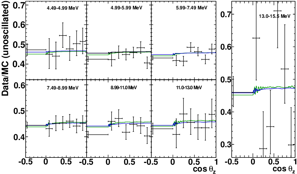
The SK-IV livetime during the day (night) is 797 days (866 days). The solar neutrino flux between 4.49 and 19.5 MeV assuming no oscillations is measured as (stat.)(sys.) /(cm2sec) during the day and (stat.)(sys.) /(cm2sec) during the night. Fig. 31 shows the solar zenith angle variation of the ratio of the measured rate to the unoscillated simulated rate (assuming /(cm2sec) for the 8B flux) in the seven energy regions shown in Table 12. Overlaid is the expected zenith variation for best-fit oscillation parameters coming from a fit to all solar neutrino data (solar+KamLAND data) in red (blue). Table 12 lists the data used in Fig. 31, the errors are statistical uncertainties only. Fig. 32 shows the data over simulated rate ratio between 4.49 and 19.5 MeV (assuming no oscillations) as a function of , divided into five day and six night bins (corresponding to the mantle 1-5 and core definitions of Table 12). By comparing the separately measured day and night fluxes, the measured day/night asymmetry for SK-IV is found to be .

| Observed Rate | Unoscillated Rate | ||||||||
|---|---|---|---|---|---|---|---|---|---|
| Energy | DAY | MANTLE1 | MANTLE2 | MANTLE3 | MANTLE4 | MANTLE5 | CORE | 8B | |
| (MeV) | |||||||||
| 167.8 | 0.323 | ||||||||
| 283.6 | 0.611 | ||||||||
| 321.4 | 0.799 | ||||||||
| 196.6 | 0.647 | ||||||||
| 122.2 | 0.619 | ||||||||
| 36.0 | 0.365 | ||||||||
| 7.45 | 0.204 | ||||||||
The SK-IV day/night asymmetry resulting from the day/night amplitude fit method, for an energy range of 4.49-19.5 MeV and oscillations parameters preferred by SK ( eV2, and ), is found to be
The expected day/night asymmetry for the above set of oscillation parameters is . For the case of a global fit to solar neutrino data and KamLAND [3], the mass squared splitting changes to eV2, and the expected day/night asymmetry goes to . However, the day/night amplitude fit measured SK-IV day/night asymmetry is only slightly reduced to
Within the LMA region, all measured values of the day/night asymmetry coming from the day/night amplitude fit are within of . If the above measurement is combined with the previous three phases of SK, the SK combined measured day/night asymmetry is
Previously, we published in [29] which was the first significant indication that matter effects influence neutrino oscillations. The slightly larger significance here is due to a somewhat larger data set.
VI Oscillation Analysis
SK measures elastic scattering of solar neutrinos with electrons, the rate of which depends on the flavor content of the solar neutrino flux, so it is sensitive to neutrino flavor oscillations. To constrain the parameters governing these oscillations, we analyze the integrated scattering rate, the recoil electron spectrum (which statistically implies the energy-dependence of the electron-flavor survival probability), and the time of the interactions which defines the neutrino path through the earth during night time, and therefore controls the earth matter effects on solar neutrino oscillations. An expansion of the likelihood used in the extended maximum likelihood fit to extract the solar neutrino signal (see section III.3) could make full use of all information (timing, spectral information and rate), but is CPU time intensive. Instead, we separate the log(likelihood) into a time-variation (day/night variation) portion and a spectral portion: where , the likelihood for assuming no time variation, is replaced by . This fits the calculated elastic scattering rate rate in energy bin of a particular SK phase to the measurement . The calculated event rate is the sum of the expeced elastic scattering rate from 8B neutrinos scaled by the parameter and from hep neutrinos scaled by the parameter : . The calculation includes neutrino flavor oscillations of three flavors; they depend on the mixing angles , and the mass squared difference . is then multiplied by the spectral distortion factor which describes the effect of a systematic shift of the 8B neutrino spectrum scaled by the constrained nuisance parameter , a deviation in the SK energy scale in phase described by the constrained nuisance parameter , and a systematic change in the SK energy resolution based on a third constrained nuisance parameter . If is the number of energy bins of phase , we minimize
over all systematic nuisance parameters and the flux scaling parameters:
| (8) |
where constrains the flux parameters to prior uncertainties: is constrained to result in a flux of /(cm2sec) (motivated by the SNO NC measurement of the total 8B neutrino flux [18]), is only slightly constrained to correspond to a hep flux of /(cm2sec). The nuisance parameters , , and are constrained to (i.e. they are defined as standard Gaussian variables) by the “penalty terms” , , and . We rewrite equation 8 as a quadratic form with the curvature matrix and the best-fit flux parameters and as
| (9) |
for . The parameter is introduced to scale the a posteriori constraints on the flux parameters by without affecting the minimum in order to take into account additional systematic uncertainties of the total rate. These uncertainties are not covered by or . Table 5 (subtotal) lists these additional uncertainties integrated over all energies. To incorporate them we choose . To best compare this three-flavor analysis to two-flavor analyses performed for previous phases, we also perform an analysis with an a priori constraint on coming from reactor neutrino experiments [26]. Unlike the two-flavor analyses, is not fixed to zero, but constrained to a non-zero value by . The time-variation likelihood is simply the difference between the likelihoods with and without the predicted day/night variation assuming the best-fit flux and nuisance parameters from the spectrum minimization. As the uncertainties in each spectral bin are closely approximated by Gaussian uncertainties, the total is then given by . Figure 33 shows allowed regions of oscillation parameters from SK-IV data with the external constraint from reactor neutrino data on at the , , , , and confidence level. SK-IV determines to be , as well as to be eV2. A secondary region appears at about the level at eV2. Small mixing is only very marginally allowed at about the confidence level.
We combined the SK-IV constraints with those of previous SK phases, as well as other solar neutrino experiments [18, 23]. For the combined SK fit, the spectrum and rate is
| (10) |
Each SK phase is represented by a separate day/night likelihood ratio, where the flux and nuisance parameters are taken from the combined fit. Fig. 33 shows the SK combined allowed areas based on rate, spectrum, and day/night variation. SK selects large mixing () over small mixing by more than five standard deviations and very strongly (3.6 ) favors the of the large mixing angle (LMA) solution (below eV2 and above eV2) over any other oscillation parameters. SK determines to be , as well as to be eV2.


Fig. 34 compares the SK+SNO combined constraints to those based on SNO data alone [18]. While SNO’s measurement of the mixing angle is more precise () than SK’s, its constraints are poorer ( eV2). Also, SNO very slightly favors the Low solution (near eV2) and allows small mixing at the 3.6 level. The combined analysis of SK and SNO is particularly powerful: as SNO and SK both measure 8B neutrinos in a very similar energy range but in a different way and with different systematic effects, the combined analysis profits from correlations and is better than a mere addition of ’s. The SK+SNO combined analysis measures and eV2. Oscillation parameter values outside the LMA are very strongly excluded: the solar mixing angle lies within at about the 7.5 C.L., eV2 (which includes the “small mixing angle” and “low” regions) is ruled out at the 5.5 C.L., and eV2 is excluded at 7.5 C.L. The hep flux constraint used by SNO is /(cm2sec) from the solar standard model [22]. The SK and SNO combined analysis also uses this tighter constraint.


The combined allowed contours based on SK, SNO [18] and other solar neutrino experiments’ [23] data, KamLAND’s constraints and the combination of the two are shown in Fig. 34 and Fig. 35. SK and SNO dominate the combined fit to all solar neutrino data. This can be seen from the two almost identical sets of green contours in Fig. 34. In the right panel of this figure, some tension between the solar neutrino and reactor anti-neutrino measurements of the solar is evident, stemming from the SK day/night measurement. Even though the expected day/night amplitude agrees within with the fitted amplitude for any , in either the KamLAND or the SK range, the SK data slightly favor the shape of the day/night variation predicted by values of that are smaller than KamLAND’s. Fig. 35 shows the results of the unconstrained fit. Solar neutrinos by themselves weakly favor a non-zero by about one standard deviation because for low energy solar neutrinos the survival probability (e.g ) is about while the MSW effect causes a high energy (8B) solar neutrino survival probability of . This results in a correlation of and for high energy neutrinos and an anti-correlation for low energy neutrinos. KamLAND reactor neutrino data has the same anti-correlation as the low energy solar neutrinos because in both cases matter effects play a minor role. Therefore the significance of non-zero increases in the solar+KamLAND data combined fit to about two , favoring .
VII Conclusion
The fourth phase of SK measured the solar 8B neutrino-electron elastic scattering-rate with the highest precision yet. SK-IV measured a solar neutrino flux of assuming no oscillations. When combined with the results from the previous three phases, the SK combined flux is ((stat.)(syst.)) /(cm2sec). A quadratic fit of the electron-flavor survival probability as a function of energy to all SK data, as well as a combined fit with SNO solar neutrino data, very slightly favor the presence of spectral distortions, but are still consistent with an energy-independent electron neutrino flavor content. The SK-IV solar neutrino elastic scattering day/night rate asymmetry is measured as ((stat.)(syst.)). Combining this with other SK phases, the SK solar zenith angle variation data gives the first significant indication for matter-enhanced neutrino oscillation. This leads SK to having the world’s most precise measurement of eV2, using neutrinos rather than anti-neutrinos. There is a slight tension of 1.5 between this value and KamLAND’s measurement using reactor anti-neutrinos. The tension increases to 1.6 , if other solar neutrino data are included. The SK-IV solar neutrino data determine the solar mixing angle as , all SK solar data measures this angle to be , the determined squared splitting is eV2. A constrained fit to all solar neutrino data and KamLAND yields and eV2. When this constraint is removed, solar neutrino experiments and KamLAND measure , a value in good agreement with reactor neutrino measurements.
VIII Acknowledgments
The authors gratefully acknowledge the cooperation of the Kamioka Mining and Smelting Company. Super-K has been built and operated from funds provided by the Japanese Ministry of Education, Culture, Sports, Science and Technology, the U.S. Department of Energy, and the U.S. National Science Foundation. This work was partially supported by the Research Foundation of Korea (BK21 and KNRC), the Korean Ministry of Science and Technology, the National Science Foundation of China (Grant NO. 11235006), the European Union H2020 RISE-GA641540-SKPLUS, and the National Science Centre, Poland (2015/17/N/ST2/04064, 2015/18/E/ST200758).
References
- [1] J. Hosaka et al., Phys. Rev. D 73, 112001 (2006).
- [2] The SNO Collaboration, Phys. Rev. Lett. 87, 071301 (2001).
- [3]
S. Abe et al., Phys. Rev. Lett. 100, 221803 (2008);
The KamLAND Collaboration, arxiv:1303.4667v2 (2013). - [4]
S. P. Mikheyev and A. Y. Smirnov, Sov. Jour. Nucl. Phys. 42, 913 (1985);
L. Wolfenstein, Phys. Rev. D 17, 2369 (1978). - [5] Y. Fukuda et al., Nucl. Instr. and Meth. A, 501 (2003) 418-462.
- [6] J. P. Cravens et al., Phys. Rev. D 78, 032002 (2008).
- [7] K. Abe et al., Phys. Rev. D 83, 052010 (2011).
- [8] H. Nishino et al., Nucl. Inst. and Meth. A 620 (2009), S. Yamada et al.IEEE Trans. Nucl. Sci. 57, 428 (2010).
- [9] M. Nakahata et al., Nucl. Instr. and Meth. A 421, 113 (1999).
- [10] E. Blaufuss et al., Nucl. Instr. and Meth. A 458, 636 (2001).
- [11] K. Abe et al., Nucl. Instr. and Meth. A 737 (2014) 253-272.
- [12] Y. Nakano, Ph. D. thesis, University of Tokyo (2016); http://www-sk.icrr.u-tokyo.ac.jp/sk/publications/index-e.html.
- [13] S. W. Li and J. F. Beacom, Phys. Rev. C 89, 045801 (2014), S. W. Li and J. F. Beacom, Phys. Rev. D 91 no.10, 105005 (2015).
- [14] Y. Zhang et al., Phys. Rev. D 93, 012004 (2016).
- [15] W. T. Winter et al., Phys. Rev. C 73, 025503 (2006).
- [16] J. N. Bahcall et al., Phys. Rev. C 54, 6146 (1995).
- [17] J. N. Bahcall et al., Phys. Rev. D 51, 6146 (1995).
- [18] B. Aharmin et al., Phys. Rev. C 88, 025501 (2013).
- [19] B. Aharmim et al., Astrophys. J. 653, 1545 (2006).
- [20] A. Friedland, C. Lunardini and C. Peña-Garay, Phys. Lett. B 594, 347 (2004).
- [21]
R. Fardon, A. E. Nelson and N. Weiner, JCAP 0410, 005 (2004);
M. Cirelli, M. C. Gonzalez-Garcia and C. Peña-Garay, Nucl. Phys. B 719, 219 (2005). - [22] J. N. Bahcall, A. M. Serenelli and S. Basu, Astrophys. J. Suppl 165, 400 (2006).
- [23]
R. Davis et al. (Homestake Experiment), Phys. Rev. Lett. 20, 1205 (1968).
J. N. Abdurashitov et al. (SAGE collaboration), Phys. Rev. C 80, 015807 (2009);
M. Altmann et al. (GALLEX Collaboration), Phys. Lett. B 616, 174 (2005);
G. Bellini et al. (Borexino Collaboration), Phys. Rev. Lett. 107, 141302 (2011). - [24] Bellini et al. Phys. Rev. D 82, 033006 (2010); Bellini et al. Phys. Rev. Lett. 108, 051302 (2012).
- [25] M. B. Smy et al., Phys. Rev. D 69, 011104(R) (2004).
- [26]
F. P. An et al., arXiv:1210.6327 (2012);
J. K. Ahn et al., Phys. Rev. Lett. 108, 191802 (2012);
Y. Abe et al., Phys. Rev. D 86, 052008 (2012). - [27] A. M. Dziewonski and D. L. Anderson, Phys. Earth Planet. Inter. 25, 297 (1981).
- [28] J. J. Durek and G. Ekstrom, Bull. Seism. Soc. Am. 86, 144-158 (1996).
- [29] A. Renshaw et al., Phys. Rev. Lett. 112, 091805 (2014).
Appendix A Revised SK-III results
Since the publication of the previous report [7], two mistakes were found. One is in how energy-dependent systematic errors are calculated and the other is related to the flux calculation in SK-III. The estimates of the energy-correlated uncertainties in the main text of that report are based on the Monte Carlo (MC) simulated 8B solar neutrino events. It is found that this evaluation method was not accurate enough. The statistical error of the MC simulation distorted the shapes of the energy-correlated uncertainties systematically.
The energy dependence of the differential interaction cross-section between neutrinos and electrons was accidentally eliminated only for the SK-III flux calculation in the main text. Figure A.1 shows the energy distributions of recoil electrons from 8B solar neutrinos.

The blue dotted histogram shows the true energy spectrum shape from a theoretical calculation considering the detector resolutions. The red solid plot shows the energy spectrum shape used in the SK-III analysis in the previous report. The expected total flux was normalized correctly, but the expected 8B energy spectrum shape was improperly distorted in the analysis.
These mistakes have been fixed in this paper. In this appendix, the revised SK-III solar neutrino results are described. The latest oscillation results, including both revised SK-III data and SK-IV data, are reported in the main text of this report.
A.1 Systematic uncertainties
The energy-correlated systematic uncertainties are obtained by counting the number of events in the solar neutrino MC simulation with artificially shifted energy scale, energy resolution and 8B solar neutrino energy spectrum. In the SK-III analysis in the previous report, this estimation was done with the generated solar neutrino MC events. However, in the high energy region, not enough MC events were generated to accurately estimate the small systematic errors. In the current analysis, this estimation is performed with a theoretical calculation considering the detector resolutions, thus eliminating the statistical effects introduced by the small MC statistics.
The revised results of the energy-correlated systematic uncertainties are shown in Fig. A.2. In this update, the uncertainty from 8B spectrum shape was improved.

| Source | Total Flux |
|---|---|
| Energy scale | |
| Energy resolution | |
| 8B spectrum | |
| Trigger efficiency | |
| Angular resolution | |
| Vertex shift | |
| Event quality cuts | |
| - Reconstruction Goodness | |
| - Hit pattern | |
| - Second vertex | |
| Spallation cut | |
| Gamma-ray cut | |
| Cluster hit cut | |
| Background shape | |
| Signal extraction | |
| Livetime | |
| Cross section | |
| Total |
| Energy | Observed Rate | Expected Rate | |||
|---|---|---|---|---|---|
| (MeV) | ALL | DAY | NIGHT | 8B | hep |
| 189.7 | 0.334 | ||||
| 172.2 | 0.321 | ||||
| 155.2 | 0.310 | ||||
| 134.3 | 0.289 | ||||
| 117.1 | 0.271 | ||||
| 101.2 | 0.257 | ||||
| 85.8 | 0.240 | ||||
| 71.7 | 0.223 | ||||
| 58.5 | 0.205 | ||||
| 47.1 | 0.186 | ||||
| 37.0 | 0.169 | ||||
| 28.5 | 0.151 | ||||
| 21.45 | 0.134 | ||||
| 15.76 | 0.118 | ||||
| 11.21 | 0.102 | ||||
| 7.79 | 0.088 | ||||
| 5.22 | 0.074 | ||||
| 3.39 | 0.062 | ||||
| 3.49 | 0.092 | ||||
| 1.227 | 0.059 | ||||
| 0.513 | 0.068 | ||||

The systematic uncertainties on total flux in SK-III are also revised. The revised uncertainties are summarized in Table A.1. The 8B spectrum error was underestimated in the analysis in the main text of [7]. The revised systematic uncertainty on the total flux in Etotal = 5.0–20.0 MeV in SK-III is estimated to be 2.2.
A.2 8B solar neutrino flux results
The observed number of solar neutrino events is also updated. In this analysis, the extracted number of 8B solar neutrinos with the ES reaction in Etotal = 5.0–20.0 MeV for a live time of 548 days of SK-III data was 8148(stat) (sys). The corresponding 8B flux is obtained to be:
Fixing the cross section problem, a 3.4% increase was observed.
Appendix B Parametrized Survival Probability Fit
We fit the SK spectral data to the exponential, quadratic, and cubic survival probability in the same manner as we fit them to the MSW prediction. Fig. B.1 shows the resulting allowed areas of the exponential coefficients and . The “baseline” (average ) is profiled; the constraint results from the comparison of the electron elastic scattering rate in SK and the SNO neutral-current interaction rate on deuterium. The contours deviate from a multivariate Gaussian. As there is no significant deviation from an undistorted spectrum, the data impose no constraint on , the “steepness” of the exponential. Table B.1 uses the best quadratic form approximation of the of the fit as a function of the parameters to extract the values, uncertainties and correlations. Fig. B.2 shows the allowed shape parameters ( and ) and the allowed slope () versus the baseline () of the quadratic fit. The SK-IV contours show some deviations from a multivariate Gaussian at , while the SK combined result is consistent with it. Overlaid in blue are the constraints from the SNO measurements. The corresponding coefficients of Table B.1 differ slightly from those in [18] which fits both the survival probability to a quadratic function and the energy dependent day/night asymmetry to a linerar function. Here, we assume the energy dependence of the day/night effect calculated from standard earth matter effects. The resulting reduction in the degree of freedom leads to somewhat tighter constraints as well as a slight shift in the best fit value. The precision of the SK constraint is similar to that based on SNO data, and also statistically consistent. Since SK’s correlation between and is opposite to that of SNO’s, a combined fit is rather powerful in constraining the shape. The correlation is slightly smaller. The addition of SK data to SNO data not only significantly increases the precision of the determination, but the uncertainties on the shape are reduced.
| Data Set | - corr. | ||||||
|---|---|---|---|---|---|---|---|
| SK-IV | no constraint | ||||||
| SK | no constraint | ||||||
| quadratic function | cubic function | ||||||
| SK-IV | |||||||
| SK | |||||||
| - corr. | - corr. | - corr. | |||||
| SNO | |||||||
| SK+SNO | |||||||


Appendix C Tables
| Energy | Observed Rate | Expected Rate | |||
|---|---|---|---|---|---|
| (MeV) | ALL | DAY | NIGHT | 8B | |
| 196.8 | 0.346 | ||||
| 182.8 | 0.335 | ||||
| 167.8 | 0.323 | ||||
| 153.3 | 0.312 | ||||
| 137.8 | 0.298 | ||||
| 121.9 | 0.282 | ||||
| 106.8 | 0.266 | ||||
| 92.1 | 0.250 | ||||
| 78.0 | 0.232 | ||||
| 65.2 | 0.214 | ||||
| 53.4 | 0.197 | ||||
| 42.9 | 0.179 | ||||
| 33.8 | 0.162 | ||||
| 26.0 | 0.144 | ||||
| 19.55 | 0.128 | ||||
| 14.34 | 0.112 | ||||
| 10.24 | 0.097 | ||||
| 7.10 | 0.083 | ||||
| 4.80 | 0.070 | ||||
| 3.11 | 0.059 | ||||
| 3.18 | 0.088 | ||||
| 1.117 | 0.056 | ||||
| 0.464 | 0.064 | ||||
Energy (MeV) SK-I SK-II SK-III SK-IV 3.49-3.99 3.99-4.49 4.49-4.99 4.99-5.49 5.49-5.99 5.99-6.49 6.49-6.99 6.99-7.49 7.49-7.99 7.99-8.49 8.49-8.99 8.99-9.49 9.49-9.99 9.99-10.5 10.5-11.0 11.0-11.5 11.5-12.0 12.0-12.5 12.5-13.0 13.0-13.5 13.5-14.5 14.5-15.5 15.5-19.5