Multiclass feature learning for hyperspectral image classification: sparse and hierarchical solutions.
Abstract
In this paper, we tackle the question of discovering an effective set of spatial filters to solve hyperspectral classification problems. Instead of fixing a priori the filters and their parameters using expert knowledge, we let the model find them within random draws in the (possibly infinite) space of possible filters. We define an active set feature learner that includes in the model only features that improve the classifier. To this end, we consider a fast and linear classifier, multiclass logistic classification, and show that with a good representation (the filters discovered), such a simple classifier can reach at least state of the art performances. We apply the proposed active set learner in four hyperspectral image classification problems, including agricultural and urban classification at different resolutions, as well as multimodal data. We also propose a hierarchical setting, which allows to generate more complex banks of features that can better describe the nonlinearities present in the data.
Keywords:
Hyperspectral imaging, active set, feature selection, multimodal, hierarchical feature extraction, deep learning.1 Introduction
Hyperspectral remote sensing allows to obtain a fine description of the materials observed by the sensor: with arrays of sensors focusing on 5-10 nm sections of the electromagnetic spectrum, hyperspectral images (HSI) return a complete description of the response of the surfaces, generally in the visible and infrared range. The use of such data, generally acquired by sensors onboard satellites or aircrafts, allows to monitor the processes occurring at the surface in a non-intrusive way, both at the local and global scale [18, 29]. The reduced revisit time of satellites, in conjunction with the potential for quick deployment of aerial and unmanned systems, makes the usage of hyperspectral systems quite appealing. As a consequence, hyperspectral data is becoming more and more prominent for researchers and public bodies.
Even if the technology is at hand and images can be acquired by different platforms in a very efficient way, HSI alone are of little use for end-users and decision makers: in order to be usable, remote sensing pixel information must be processed and converted into maps representing a particular facet of the processes occurring at the surface. Among the different products traditionally available, land cover maps issued from image classification are the most common (and probably also the most used). In this paper, we refer to land cover/use classification as the process of attributing a land cover (respectively land use) class to every pixel in the image. These maps can then be used for urban planning [32, 33], agriculture surveys [1] or surveying of deforestation [2, 21, 37].
The quality of land cover maps is of prime importance. Therefore, a wide panel of research works consider image classification algorithms and their impact on the final maps [26, 7, 20, 6]. Improving the quality of maps issued from HSI is not trivial, as hyperspectral systems are often high dimensional (number of spectral bands acquired), spatially and spectrally correlated and affected by noise [6]. Among these peculiarities of remote sensing data, spatial relations among pixels have received particular attention [11]: the land cover maps are generally smooth, in the sense that neighboring pixels tend to belong to the same type of land cover [30]. On the contrary, the spectral signatures of pixels of a same type of cover tend to become more and more variable, especially with the increase of spatial resolution. Therefore, HSI classification systems have the delicate task of describing a smooth land cover using spectral information with a high within-class variability. Solutions to this problem have been proposed in the community and mostly recur to spatial filtering that work at the level of the input vector [4, 38, 11] or to structured models that work by optimization of a context-aware energy function [31, 30, 19].
In this paper, we start from the first family of methods, those based on the extraction of spatial filters prior to classification. Methods proposed in remote sensing image classification tend to pre-compute a large quantity of spatial filters related to the user’s preference and knowledge of the problem: texture [23], Gabor [17], morphological [4, 10] or bilateral filters [30] are among those used in recent literature and we will use them as buiding blocks for our system. With this static and overcomplete set of filters (or filterbank), a classifier is generally trained.
Even if successful, these studies still rely on the definition -priori of a filterbank. This filterbank depends on the knowledge of the analyst and on the specificities of the image at hand: a pre-defined filterbank may or may not contain the filters leading to the best performances. A filterbank constructed -priori is also often redundant: as shown in Fig. 1, the filter bank is generally applied to each band of the image, resulting into a -dimensional filter bank, where is the number of filters and the number of bands. Proceeding this way proved in the past to be unfeasible for high dimensional datasets, such as hyperspectral data, for which the traditional way to deal with the problem is to perform a principal components analysis (PCA) and then extract the filters from the principal components related to maximal variance [4]. In that case, the final input space becomes -dimensional. A first problem is related during this dimension reduction phase, for which the choice of the feature extractor and of the number of features remains arbitrary and may lead to discarding information that is discriminative, but not related to large variance. Therefore, a first objective of our method is to avoid this first data reduction step. But independently to the reduction phase, this goes against the desirable property of a model to be compact, i.e., to depend on as few input variables as possible. Therefore, in most works cited above an additional feature selection step is run to select the most effective subset for classification. This additional step can be a recursive selection [35] or be based on kernel combination [34], on the pruning of a neural network [23] or on discriminative feature extraction [4].
Proceeding this way is suboptimal in two senses: first, one forces to restrict the number and parameters of filters to be used to a subset, whose appropriateness only depends on the prior knowledge of the user. In other words, the features that are relevant to solve the classification problem might not be in the original filterbank. Second, generating thousands of spatial filters and use them all together in a classifier, that also might operate with a feature selection strategy, increases the computational cost significantly, and might even deteriorate the classification accuracy because of the curse of dimensionality. Note that, if the spatial filters considered bear continuous parameters (e.g. Gabor or angular features), there is theoretically an infinite number of feature candidates.
This paper tackles these two problems simultaneously: instead of pre-computing a specific set of filters, we propose to interact with the current model and retrieve only new filters that will make it better. These candidate filters can be of any nature and with parameters unrestricted, thus allowing to explore the (potentially infinite) space of spatial filters. This leads to an integrated approach, where we incrementally build the set of filters from an empty subset and add only the filters improving class discrimination. This way of proceeding is of great interest for automatic HSI classification, since the filters are selected automatically among a very large set of possible ones, and are those that best fit the problem at hand.
Two approaches explored similar concepts in the past: Grafting [25] and Group Feature Learning [28], which incrementally select the most promising feature among a batch of features extracted from the universe of all possible features admitted. Since this selection is based on a heuristic criterion ranking the features by their informativeness when added to the model, it may be seen as performing active learning [9] in the space of possible features (in this case, the active learning oracle is replaced by the optimality condition, for which only the features improving the current classifier are selected).
| (a) Proposed AS-Bands | (b) Proposed ASH-Bands |
In this paper, we propose a new Group Feature Learning model based on multiclass logistic regression (also known as multinomial regression). The use of a group-lasso regularization [39] allows to jointly select the relevant features and also to derive efficient conditions for evaluating the discriminative power of a new feature. In Rakotomamonjy et al. [28], authors propose to use group-lasso for multitask learning by allowing to use an additional sparse average classifier common to all tasks. Adapting their model in a multiclass classification setting leads to the use of the sole group-lasso regularization. Note that one could use a support vector machine as in Tuia et al. [36] to select the relevant feature in a One-VS-All setting, but this approach is particularly computationally intensive, as the incremental problem is solved for each class separately. This implies the generation of millions of features, that may be useful for more than one class at a time. To achieve an efficient multiclass strategy, we propose the following three original contributions:
- 1.
We use here a multiclass logistic classifier (MLC) with a softmax loss. MLC allows to natively handle several classes without using the One-VS-All approach and has the advantage of providing probabilistic prediction scores that can more easily be used in structured models (such as Markov random fields).
- 2.
We employ a group lasso regularization, which allows to select features useful for many classes simultaneously, even if they do not show the highest score for a single class. This means sharing information among the classes, similarly to what would happen in a multitask setting [16]. This model, called AS-Bands, is detailed in Fig. 2(a).
- 3.
We investigate the automatic selection of complex hierarchical spatial filters built as modifications of previously selected filters. This leads to a tree- (or graph-) based feature extraction that can encode complex nonlinear relationship for each class. Such a hierarchical re-processing of features has connections with deep neural networks [14, 15], which have recently proven to be able to improve significantly the performance of existing classification methods in computer vision [8, 13]. This model, called ASH-bands, is detailed in Fig. 2(b).
We test the proposed method on two landcover classification tasks with hyperspectral images of agricultural areas and on one landuse classification example over an urban area exploiting jointly hyperspectral and LiDAR images. In all cases, the proposed feature learning method solves the classification tasks with at least state of the art numerical performances and returns compact models including only features that are discriminative for more than one class. Among the two method proposed, the hierarchical feature learning tends to outperform the shallow feature extractor for traditional classification problems. However, when confronted to shifting distributions between train and test (i.e. a domain adaptation problem), it provides slightly worse performances, probably due to the complexification of the selected features, that overfit the training examples.
The remainder of this paper is as follows: Section 2 details the proposed method, as well as the multiclass feature selection using group-lasso. In Section 3 we present the datasets and the experimental setup. In Section 4 we present and discuss the experimental results. Section 5 concludes the paper.
2 Multiclass active set feature discovery
In this section, we first present the multiclass logistic classification and then derive its optimality conditions, which are used in the active set algorithm.
2.1 Multiclass logistic classifier with group-lasso regularization
Consider an image composed of pixels . A subset of pixels is labeled into one of classes: , where are integer values . We consider a (possibly infinite) set of -parametrized functions mapping each pixel in the image into the feature space of the filter defined by . As in Tuia et al. [36], we define as the set of all possible finite subsets of features and as an element of composed of features . We also define as the stacked vector of all the values obained by applying the filters to pixel and the matrix containing the features in computed for all the labeled pixels. Note that in this work, we suppose that all the features have been normalized with each column in matrix having a unit norm.
In this paper we consider the classification problem as a multiclass logistic regression problem with group-lasso regularization. Learning such a classifier for a fixed amount of features corresponds to learning a weight matrix and the bias vector using the softmax loss. In the following, we refer to as the weights corresponding to class , which corresponds to the -th column of matrix . The -th line of matrix is denoted as . The optimization problem for a fixed feature set is defined as:
| (1) |
where the first term corresponds to the soft-max loss with defined as
and the second term is a group-lasso regularizer. In this paper, we use the weighted mixed norm :
| (2) |
where the coefficients correspond to the weights used for regularizing the th feature. Typically one want all features to be regularized similarly by choosing . However, in the hierarchical feature extraction proposed in Section 2.3 we will use different weights in order to limit over-fitting when using complex hierarchical features.
This regularization term promotes group sparsity, due to its non differentiability at the null vector of each group. In this case we grouped the coefficients of by lines, meaning that the regularization will promote joint feature selection for all classes. Note that this approach can be seen as multi-task learning where the tasks corresponds to the classifier weights of each class [22, 27]. As a result, if a variable (filter) is active, it will be active for all classes. This is particularly interesting in in a multiclass setting, since a feature that helps in detecting a given class also helps in “not detecting” the others classes: for this reason a selected feature should be active for all the classifiers.
The algorithm proposed to solve both the learning problem and feature selection is derived from the optimality conditions of the optimization problem of Eq. (1). Since the problem defined in Eq. (1) is non-differentiable, we compute the sub-differential of its cost function:
| (3) |
where the first term corresponds to the gradient of the softmax data fitting and the second term is the sub-differential of the weighted group lasso defined in Eq. (2). is a matrix that, for a given sample and a class , equals:
| (4) |
where and if and 0 otherwise. In the following, we define as a matrix corresponding to the gradient of the data fitting term w.r.t . Note that this gradient can be computed efficiently with multiple scalar product between the features and the multiclass residual . The optimality conditions can be obtained separately for each , i.e. for each line of the matrix. consists in a weighted sum of non differentiable norm-based regularization [3]. The optimality condition for the norm consists in a constraint with its dual norm (namely itself):
| (5) |
which in turn breaks down to:
| (6) |
These optimality conditions show that the selection of one variable, i.e. one group, can be easily tested with the second condition of equation (6). This suggests the use of an active set algorithm. Indeed, if the norm of correlation of a feature with the residual matrix is below , it means that this feature is not useful for classification and its weight will be set to for all the classes. On the contrary, if not, then the group can be defined as “active” and its weights have to be estimated.
2.2 Proposed active set criterion (AS-bands)
We want to learn jointly the best set of filters and the corresponding MLC classifier. This is achieved by minimizing Eq. (1) jointly on and . As in Rakotomamonjy et al. [28], we can extend the optimality conditions in (6) to all filters with zero weights that are not included in the current active set :
| (7) |
Indeed, if this constraint holds for a given feature not in the current active set, then adding this feature to the optimization problem will lead to a row of zero weights for this feature. But this also means that if we find a feature that violates Eq. (7), its inclusion in will (after re-optimization) make the global MLC cost decrease and provide a feature with non-zero coefficients for all classes.
The pseudocode of the proposed algorithm is given in Algorithm 1: we initialize the active set with the spectral bands and run a first MLC minimizing Eq. (1). Then we generate a random minibatch of candidate features, , involving spatial filters with random types and parameters. We then assess the optimality conditions with (7): if the feature with maximal is greater than , it is selected and added to the current active set . After one feature is added the MLC classifier is retrained and the process is iterated using the new active set.
Inputs
- Bands to extract the filters from ()
- Initial active set
2.3 Hierarchical feature learning (ASH-bands)
Algorithm 1 searches randomly in a possibly infinite dimensional space corresponding to all the possible spatial filters computed on the input bands. But despite all their differences, the spatial filters proposed in the remote sensing community (see, as an example, those in Tab. 4) can yield only a limited complexity and non-linearity. When the classes are not linearly separable, learning a linear classifier may require a large number of these relatively simple features. In this section we investigate the use of hierarchical feature generation that can yield much more complex data representation and therefore hopefully decrease the number of features necessary for a good classification.
Hierarchical feature extraction is obtained by adding the already selected features in the pool of images that can be used for filtering at the next feature generation step. Using a retained filter as a new possible input band leads to more complex filters with higher nonlinearity. This is somehow related to the methods of deep learning, where deep features are generally obtained by aggregation of convolution operators. In our case, those operators are substituted by spatial filters with known properties, which adds up to our approach the appealing property of direct interpretability of the discovered features. In deep learning models, interpretation of the features learned is becoming possible, but at the price of series of deconvolutions [40]. Let be the depth of a given feature , with 0 being the depth of original features: this is the number of filtering steps the original bands has undergone to generate filter . For example, the band 5 has depth , while the filters that are issued from this band, for example a filter issued from an opening computed on band 5, will have depth . If the opening band is then re-filtered by a texture filter into a new filter , its depth will be . This leads to a much more complex feature extraction that builds upon an hierarchical, tree-shaped, suite of filters. The depth of the feature in the feature generation tree is of importance in our case since it is a good proxy of the complexity of the features. In order to avoid over-fitting, we propose to regularize the features using their depth in the hierarchy. As a criterion, we use a regularization weight of the form , with being a term penalizing depth in the graph.
The proposed hierarchical feature learning is summarized in Algorithm 2.
Inputs
- Bands to extract the filters from () with depth
- Initial active set
3 Data and setup of experiments
In this section, we present the three datasets used, as well as the setup of the four experiments considered.
3.1 Datasets
We studied the proposed active set method on four hyperspectral classification tasks, involving two crops identification datasets and one urban land use dataset (considered in two ways):
- a)
Indian Pines 1992 (AVIRIS spectrometer, HS): the first dataset is a 20-m resolution image taken over the Indian Pines (IN) test site in June 1992 (see Fig. 3). The image is pixels and contains 220 spectral bands. A ground survey of 10366 pixels, distributed in 16 crop types classes, is available (see Table 1). This dataset is a classical benchmark to validate model accuracy. Its challenge resides in the strong mixture of the classes’ signatures, since the image has been acquired shortly after the crops were planted. As a consequence, all signatures are contaminated by soil signature, making thus a spectral-spatial processing compulsory to solve the classification problem. As preprocessing, 20 noisy bands covering the region of water absorption have been removed.
Table 1: Classes and samples () of the ground truth of the Indian Pines 1992 dataset (cf. Fig. 3). Class Class Alfalfa 54 Oats 20 Corn-notill 1434 Soybeans-notill 968 Corn-min 834 Soybeans-min 2468 Corn 234 Soybeans-clean 614 Grass/Pasture 497 Wheat 212 Grass/Trees 747 Woods 1294 Grass/Past.-mowed 26 Towers 95 Hay-windrowed 489 Other 380 Total 10366 

(a) (b) Figure 3: Indian Pines 1992 AVIRIS data.(a) False color composition and (b) ground truth (for color legend, see Tab. 1). Unlabeled samples are in black. - b)
Indian Pines 2010 (ProSpecTIR spectrometer, VHR HS): the second dataset considers multiple flightlines acquired near Purdue University, Indiana, on May 24-25, 2010 by the ProSpecTIR system (Fig. 4). The image subset analyzed in this study contains 445750 pixels at 2m spatial resolution, with 360 spectral bands of 5nm width. Sixteen land cover classes were identified by field surveys, which included fields of different crop residue, vegetated areas, and man-made structures. Many classes have regular geometry associated with fields, while others are related with roads and isolated man-made structures. Table 2 shows class labels and number of training samples per class.


(a) (b) Figure 4: Indian Pines 2010 SpecTIR data.(a) RGB composition and (b) ground truth (for color legend, see Tab. 2). Unlabeled samples are in black. Table 2: Classes and samples () of the ground truth of the Indian Pines 2010 dataset (cf. Fig. 4). Class Class Corn-high 3387 Hay 50045 Corn-mid 1740 Grass/Pasture 5544 Corn-low 356 Cover crop 1 2746 Soy-bean-high 1365 Cover crop 2 2164 Soy-bean-mid 37865 Woodlands 48559 Soy-bean-low 29210 Highway 4863 Residues 5795 Local road 502 Wheat 3387 Buildings 546 Total 198074 - c)
Houston 2013 (CASI spectrometer VHR HS + LiDAR data). The third dataset depicts an urban area nearby the campus of the University of Houston (see Fig. 5). The dataset was proposed as the challenge of the IEEE IADF Data Fusion Contest 2013 [24]. The hyperspectral image was acquired by the CASI sensor (144 spectral bands at 2.5m resolution). An aerial LiDAR scan was also available: a digital surface model (DSM) at the same resolution as the hyperspectral image was extracted, coregistered and used as an additional band in the input space. Fifteen urban land-use classes are to be classified (Tab. 3). Two preprocessing steps have been performed: 1) histogram matching has been applied to the large shadowed area in the right part of the image (cf. Fig 5), in order to reduce domain adaptation problems [6], which are not the topic of this study: the shadowed area has been extracted by segmenting a near-infrared band and the matching with the rest of the image has been applied; 2) A height trend has been removed from the DSM, by applying a linear detrending of 3m from the West along the x-axis. Two classification experiments were performed with this data:
- (a)
Houston 2013A: we consider the left part of the image, which is unaffected by the cloud shadow. This corresponds to an image of size () pixels. The same subsampling was applied to the LiDAR DSM. The whole ground truth within the red box in Figure 5c was used to extract the train and test samples.
- (b)
Houston 2013B: the whole image was considered. Separate training and test set (in green and red in Fig. 5d, respectively), are considered instead of a random extraction. In this case, even though the projected shadow has been partially corrected by the local histogram matching, some spectral drift remains between the test samples (some of which are under the shadow) and the training ones (which are only in the illuminated areas). This was the setting of the IEEE IADF Data Fusion Contest 2013 and aimed at classification under dataset shift [6]. This problem is much more challenging than Houston 2013A and we use it as a benchmark against the state of the art, i.e. the results of the contest. However, remind that our method is not designed to solve domain adaptation problems explicitly.
(a) CASI image after local histogram matching 
(a) Detrended LiDAR DSM [m] 
(c) Ground truth 
(d) Training samples (green) vs test samples (red) 
Figure 5: Houston 2013.(a) RGB composition of the CASI data, (b) DSM issued from the LiDAR point cloud and (c) train and test ground truths. (for color legend, see Tab. 2). The area in the red box of the (c) panel has been used in the Houston2013A experiment, while the whole area has been used in the Houston2013B experiment, with (d) a training/test separation shown in the last panel (green: training, red: test). Unlabeled samples are in black. Table 3: Classes and samples () of the ground truth of the Houston 2013 dataset (cf. Fig. 5). Class Class Healthy grass 1231 Road 1219 Stressed grass 1196 Highway 1224 Synthetic grass 697 Railway 1162 Trees 1239 Parking Lot 1 1233 Soil 1152 Parking Lot 2 458 Water 325 Tennis Court 428 Residential 1260 Running Track 660 Commercial 1219 Total 14703 - (a)
3.2 Setup of experiments
For every dataset, all the features have been mean-centered and normalized to unit norm. This normalization is mandatory due to the optimality conditions, which is based on a scalar product (thus depending linearly on the norm of the feature).
In all the experiments, we use the multiclass logistic classifier (MLC) with norm implemented in the SPAMS package11 1 http://spams-devel.gforge.inria.fr/. We start by training a model with all available bands (plus the DSM in the Houston2013A/B case) and use its result as the first active set. Therefore, we do not reduce the dimensionality of the data prior to the feature generation. Regarding the active set itself, we used the following parameters:
- -
The stopping criterion is a number of iterations: in the Pines 1992, 2010 and Houston 2013 B and in the Houston 2013A case (the difference explained by faster convergence in the last dataset).
- -
A minibatch is composed of filters extracted from bands, randomly selected. In the Houston 2013A/B case, the DSM is added to each minibatch.
- -
The possible filters are listed in Tab. 4. Structuring elements () can be disks, diamonds, squares or lines. If a linear structuring elements is selected, an additional orientation parameter is also generated (). These filters are among those generally used in remote sensing hyperspectral classification literature (see Fauvel et al. [11]), but any type of spatial or frequency filter, descriptor or convolution can be used in the process.
- -
A single minibatch can be used twice (i.e. once a first filter has been selected, it is removed and Eq. (7) is re-evaluated on the remaining filters after re-optimization of the MLC classifier).
| Filter | ||
|---|---|---|
| Morphological | ||
| - | Opening / closing | , , |
| - | Top-hat opening / closing | , , , |
| - | Opening / closing by reconstruction | , , , |
| - | Opening / closing by reconstruction top-hat | , , , |
| Texture | ||
| - | Average | , |
| - | Entropy | , |
| - | Standard deviation | , |
| - | Range | , |
| Attribute | ||
| - | Area | , Area threshold |
| - | Bounding box diagonal | , Diagonal threshold |
| Band combinations | ||
| - | Simple ratio | |
| - | Normalized ratio | |
| - | Sum | |
| - | Product | |
In each experiment, we start by selecting an equal number of labeled pixels per class : we extracted 30 random pixels per class in the Indian Pines 1992 case, in the Indian Pines 2010 and in the Houston 2013A/B case22 2 When the number of pixels available was smaller than , we extracted 80% for training and left the rest for testing. The difference in the amount of labeled pixels per class is related to i) the amount of labeled pixels available per task and ii) the complexity of the problem at hand. As test set, we considered all remaining labeled pixels, but disregard those in the spatial vicinity of the pixels used for training. In the Indian Pines 1992 case, we consider all labeled pixels out of a window around the training pixels, in the Indian Pines 2010 case a window and in the Houston 2013A case a window. The difference is basically related to the images spatial resolution. In the Houston 2013B case, a spatially disjoint test set was provided in a separate file and was therefore used for testing purposes without spatial windowing.
When considering the hierarchical model ASH-bands, every feature that is added to the active set is also added to the input bands (see line of Algorithm 2). In order to penalize overcomplex deep features, we considered , where is the depth of the feature defined in Section 2.3. When adding filters issued from two inputs (as, for example, band ratios) .
Each experiment was repeated times, by random sampling of the initial training set (the test set also varies in the Indian Pines 1992/2010 and Houston 2013A datasets, since it depends on the specific location of the training samples). Average performances, along with their standard deviations, are reported.
4 Results and discussion
In this section, we present and discuss both the numerical results obtained and the feature selected in the AS-Bands (shallow) and ASH-Bands (deep) algorithms.
4.1 Performances along the iterations
AS-Bands: Numerical results for the three datasets in the AS-Bands (shallow) setting are provided in Fig. 6: the left column illustrates the evolution of the Kappa statistic [12] along the iterations and for three levels of regularization : the higher the parameter, the sparser the model (and the harder to violate the optimality conditions). The right column of Fig. 6 shows the evolution of the number of features in the active set.
For all the datasets, the iterative feature learning corresponds to a continuous, almost monotonic, increase of the performance. This is related to the optimality conditions of Eq. (1): each time the model adds one filter to , the MLC cost function decreases while the classifier performances raises. Overfitting is prevented by the group-lasso regularization: on the one hand this regularizer promotes sparsity through the norm, while on the other hand it limits the magnitude of the weight coefficients and promotes smoothness of the decision function by the use of the norm. Note that for the Houston 2013B dataset, the final classification performance is at the same level as the one of the winners of the contest, thus showing the ability of our approach to compete with state of the art methods.
| Indian Pines 1992 | |
| Indian Pines 2010 | |
| Houston 2013A | |
| Houston 2013B | |
For each case study, the model with the lowest sparsity () shows the initial best performance (it utilizes more features, as shown in the right column) and then keeps providing the best performances. However, the model with has an initial sparser solution and shows a steeper increase of the curve in the first iterations. When both models provide similar performance, they are actually using the same number of features in all cases. The sparsest model (, black line) shows the worst results in two out of the three datasets and in general is related to less features selected: our interpretation is that the regularization () is too strong, leading to a model that discards relevant features and is too biased for a good prediction (even when more features are added). As a consequence, the learning rate may be steeper than for the other models, but the model does not converge to an optimal solution.
| Indian Pines 1992 | |
| Indian Pines 2010 | |
| Houston 2013A | |
| Houston 2013B | |
| Method | Pines 1992 | Pines 2010 | Houston 2013A | Houston 2013B | ||
|---|---|---|---|---|---|---|
| No spatial info | MLC- | |||||
| (baseline) | # features | |||||
| MLC- | ||||||
| # features | ||||||
| Spatial info | AS-bands | |||||
| from bands | # features | |||||
| (proposed) | ASH-bands | |||||
| # features | ||||||
| Spatial info from | MLC- | |||||
| three top PCs | # features | |||||
| (baseline) | MLC- | |||||
| # features | 269 | |||||
| Spatial info from | AS-pcs | |||||
| all PCs | # features | |||||
| (proposed) | ASH-pcs | |||||
| # features | ||||||
ASH-Bands: The performance of ASH-Bands are compared to those of AS-Bands in Fig. 7. The case of is shown (the blue curves of Fig. 7 correspond to the blue curves of Fig. 6). From this comparison, two tendencies can be noticed: on the one hand, ASH-Bands shows better learning rates when the classification problem is fixed (i.e., no spectral shifts are observed between the training and test data: Indian Pines 1992, Indian Pines 2010 and Houston 2013A): by constructing more complex features, ASH-Bands can solve the classification problem in a more accurate way and without increasing substantially the size of the model (both AS-Bands and ASH-Bands show similar number of active features during the process). On the other hand, in the Houston 2013B case ASH-Bands is outperformed by the shallow model AS-Bands by in . The variance of the single runs is also significantly higher (see, the ASH-Bands row for this dataset in Tab. 5). We interpret this slower learning rate by an overfitting of the training data in the presence of dataset shift: since the test distribution is different that the one observed in training (by the projected cloud in the hyperspectral data), the spatial filters learned seem to become too specialized in explaining the training data and are then less accurate in the case of the (shifted) test distribution. Such behavior has been documented before in deep learning literature, especially when little training examples are used to learn the features [5]. Note that the classification performance is still on average.
4.2 Numerical performances at the end of the feature learning
Comparisons with competing strategies where the MLC classifier is learned on pre-defined feature sets are reported in Table 5. First, we discuss the performance of our active set approach when learning the filters applied on the original bands (AS-Bands and ASH-Bands): in the Indian Pines 1992 case, the AS- methods obtain average Kappas of using features and using features, respectively. This is a good result if compared to the upper bound of obtained by a classifier using the complete set of morphological and attribute features extracted from each spectral band (result not reported in the table)33 3 Only squared structuring elements were used and the filter size range was pre-defined by expert knowledge.. On both the Indian Pines 2010 and Houston 2013A datasets, the AS-Bands method provided average Kappa of . ASH-Bands provided comparable results, on the average more accurate, but still in the standard deviation range of the shallow model. The exception is the last dataset, Houston 2013B, for which the shallow model provides a Kappa of 0.93, while the hierarchical model is less accurate, as discussed in the previous section.
We compared these results to those obtained by classifiers trained on fixed raw bands (MLC) or on sets of morphological and attribute filters extracted form the three first principal components (MLC-). We followed the generally admitted hypothesis that the first(s) principal component(s) contain most of the relevant information in hyperspectral images [4]. On all the datasets, the proposed AS-bands method performs remarkably well compared with models using only the spectral information (MLC-) and compares at worse equivalently (and significantly better in the Indian Pines 2010 and Houston 2013B cases) with models using classifiers (thus without sparsity) and three to four times more features including spatial information (MLC-). The good performance of the method on the Indian Pines 1992 dataset (Kappa observed of ) is probably due to the application of the PCA transform prior to classification, which, besides allowing to decrease the dimensionality of the data, also decorrelates the signals and isolates the bare soil reflectance, which is present for almost all classes (cf. the data description in Section 3). For this reason, we also investigated a variant of our approach where, instead of working on the original spectral space, we used all the principal components extracted from the original data (AS-PCs and ASH-PCs). In the Indian Pines 1992 case, the increase in performance is striking, with a final Kappa of . For the three other datasets, the results remain in the same range as for the AS-bands results.
4.3 Multiclass selection
For the four images, the active set models end up with a maximum of features, shared by all classes. This model is very compact, since it corresponds to only of the initial dimensionality of the spectra. Due to the group-lasso regularization employed, the features selected are active for several classes simultaneously, as shown in Fig. 8, which illustrates the matrix for the Indian Pines 2010 and Houston 2013B experiments. The matrices correspond to those at the end of the feature learning, for one specific run of AS-Bands with . In both plots, each column corresponds to a feature selected by the proposed algorithm and each row to one class; the color corresponds to the strength of the weight (positive or negative). One can appreciate that the selected features (columns) have large coefficients – corresponding to strong green or brown tones in the figures – for more than one class (the rows).

|

|
4.4 Features visualization in AS-Bands
Figure 9 illustrates some of the features selected by AS-Bands in the Houston 2013B case. Each column corresponds to a different zoom in the area and highlights a specific class. We visualized the features of the same run as the bottom row of Fig. 8 and visualized the six features with highest , corresponding to those active for most classes with the highest squared weights. By analysis of the features learned, one can appreciate that they clearly are discriminative for the specific classification problem: this shows that, by decreasing the overall loss, adding these features to the active set really improves class discrimination.
| Class | Soil | Tennis c. | Run track | Parking 2 | Residential | Str. grass | Road | Water |
|---|---|---|---|---|---|---|---|---|
| RGB |  |
 |
 |
 |
 |
 |
 |
 |
| GT |  |
 |
 |
 |
 |
 |
 |
 |
| Classification (AS-bands) |  |
 |
 |
 |
 |
 |
 |
 |
| Feature: 31 Entropy, Band 145 (Lidar) Active in 11 classes |  |
 |
 |
 |
 |
 |
 |
 |
| Feature: 11 Attribute area Band 145, 7010 pix. Active in 11 classes |  |
 |
 |
 |
 |
 |
 |
 |
| Feature: 12 Attribute area Band 68, 2010 pix. Active in 12 classes |  |
 |
 |
 |
 |
 |
 |
 |
| Feature: 3 Closing, diamond Band 110, Active in 11 classes |  |
 |
 |
 |
 |
 |
 |
 |
| Feature: 46 Closing rec. top hat Band 106, Active in 5 classes |  |
 |
 |
 |
 |
 |
 |
 |
 |
|
 |
 |
| (a) Pines 2010 | (b) Houston 2013A |
4.5 Role of the features issued from the hierarchical model ASH-Bands
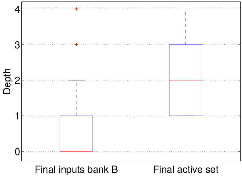
Finally, we study in detail the hierarchical features that have been discovered by our method. First, we discuss the distribution of the depth of features in the active set in the ASH-Bands model. Top row of Fig. 10 shows the distribution of the weights of the features in both the inputs bank and in the active set at the end of the feature learning. Regarding the final bank , which contains features in the Indian Pines 2010 and in the Houston 2013A case, most of the features are of depth (the original features), and . But if we consider the final active set , of size (Indian Pines 2010) and (Houston 2013A), we see that the median depth is of in both cases: this means that no features of depth (no original features) are kept in the final active set. The only exception is provided by the LiDAR data in the Houston 2013A dataset, which is kept in the final active set. These observations are confirmed by the distributions illustrated in the bottom row of Fig. 10: the distribution of depths in the final bank (blue dashed line) has 60-70% of features of depth , while the distribution of the features selected during the iterations (green line with circle markers) shows an average more towards a depth of . The features in the final active set (red line) show a distribution even more skewed towards higher depth levels, showing that features of low depth (typically depths of ) are first added to and then replaced by features with higher depth issued from them.
To confirm this hypothesis even further, we study some of the features in the final active set, illustrated in Fig. 11: when considering features of higher depth, we can appreciate the strong nonlinearity induced by the hierarchical feature construction, as well as the fact that intermediary features (the original band 105 or the features of depth 2) are discarded from the final model, meaning that they became uninformative during the process, but were used as basis to generate other features that were relevant. Another interesting behavior is the bifurcation observed in these features: the entropy filter on band 105 was re-filtered in two different ways, and ended up providing two very complementary, but informative filters to solve the problem.
| Four depth levels | |||
 Depth 0
Original band
Band 105
Depth 0
Original band
Band 105
|
|||
 In the active set
Depth 1
Entropy filter
Local window, 15 pixels
In the active set
Depth 1
Entropy filter
Local window, 15 pixels
|
|||
 |
Depth 2 Closing by reconstruction Square SE, 13 pixels |  |
Depth 2 Entropy filter Local window 15 pixels |
 |
In the active set Depth 3 Closing by reconstruction top-hat Square SE, 21 pixels |  |
In the active set Depth 3 Opening by reconstruction Square SE, 17 pixels |
| Three depth levels | |||
 |
Depth 0 Original band Band 72 |  |
Depth 0 Original band Band 93 |
 |
Depth 1 Closing by reconstruction top-hat Square SE, 19 pixels |  |
Depth 1 Closing by reconstruction Disk SE, 15 pixels |
 |
In the active set Depth 2 Opening by reconstruction Square SE, 11 pixels |  |
In the active set Depth 2 Closing by reconstruction top-hat Disk SE, 21 pixels |
| Two depth levels (as in the shallow setting) | |||
 |
In the active set Depth 0 Original band Band 145 (LiDAR) |  |
Depth 0 Original band Band 110 |
 |
In the active set Depth 1 Attribute filters - area Area of 3010 pixels |  |
In the active set Depth 1 Attribute filters - area Area of 3010 pixels |
5 Conclusions
In this paper, we proposed an active set algorithm to learn relevant features for spatio-spectral hyperspectral image classification. Confronted to a set of filters randomly generated from the bands of the hyperspectral image, the algorithm selects only those that will improve the classifier if added in the current input space. To do so, we exploit the optimality conditions of the optimization problem with a regularization promoting group-sparsity. We also propose a hierarchical extension, where active features (firstly bands and then also previously selected filters) are used as inputs, thus allowing for the generation of more complex, nonlinear filters. Analysis of four hyperspectral classification scenarios confirmed the efficiency (we use a fast and linear classifier) and effectiveness of the approach. The method is fully automatic, can include the user favorite types of spatial or frequency filters and can accommodate multiple co-registered data modalities.
In the future, we would like to extend the hierarchical algorithm to situations, where a datasets shift has occurred between the training and testing distribution: we observed that the proposed hierarchical algorithm yields lower performances on data with spectral distortion between training and test data, as in the Houston 2013B dataset. Moreover, connections to deep neural nets can be better formalized and lead to more principled way of exploring and choosing the features.
Acknowledgements
This work has been supported by the Swiss National Science Foundation (grant PP00P2_150593) and by a visiting professor grant from EPFL. We would like to thank the Image Analysis and Data fusion Technical Committee of the IEEE Geoscience and Remote Sensing Society, as well as Dr. S. Prasad, for providing the Houston data.
References
References
- Alcantara et al. [2012] Alcantara, C., Kuemmerle, T., Prishchepov, A. V., Radeloff, V. C., 2012. Mapping abandoned agriculture with multi-temporal MODIS satellite data. Remote Sens. Enviro. 124, 334–347.
- Asner et al. [2005] Asner, G. P., Knapp, D. E., Broadbent, E. N., Oliveira, P. J. C., Keller, M., Silva, J. N., 2005. Ecology: Selective logging in the Brazilian Amazon. Science 310, 480–482.
- Bach et al. [2011] Bach, F., Jenatton, R., Mairal, J., Obozinski, G., 2011. Convex optimization with sparsity-inducing norms. In: Optimization for Machine Learning. MIT Press.
- Benediktsson et al. [2005] Benediktsson, J. A., Palmason, J. A., Sveinsson, J. R., 2005. Classification of hyperspectral data from urban areas based on extended morphological profiles. IEEE Trans. Geosci. Remote Sens. 43 (3), 480–490.
- Bengio [2012] Bengio, Y., 2012. Deep learning of representations for unsupervised and transfer learning. J. Mach. Learn. Res. 27, 17–37.
- Camps-Valls et al. [2014] Camps-Valls, G., Tuia, D., Bruzzone, L., Benediktsson, J. A., 2014. Advances in hyperspectral image classification. IEEE Signal Proc. Mag. 31, 45–54.
- Camps-Valls et al. [2011] Camps-Valls, G., Tuia, D., Gómez-Chova, L., Jimenez, S., Malo, J., 2011. Remote Sensing Image Processing. Synthesis Lectures on Image, Video, and Multimedia Processing. Morgan and Claypool.
- Chatfield et al. [2014] Chatfield, K., Simonyan, K., Vedaldi, A., Zisserman, A., 2014. Return of the devil in the details: Delving deep into convolutional nets. In: British Machine Vision Conference.
- Crawford et al. [2013] Crawford, M. M., Tuia, D., Hyang, L. H., 2013. Active learning: Any value for classification of remotely sensed data? Proc. IEEE 101 (3), 593–608.
- Dalla Mura et al. [2010] Dalla Mura, M., Atli Benediktsson, J. A., Waske, B., Bruzzone, L., 2010. Morphological attribute profiles for the analysis of very high resolution images. IEEE Trans. Geosci. Remote Sens. 48 (10), 3747–3762.
- Fauvel et al. [2013] Fauvel, M., Tarabalka, Y., Benediktsson, J. A., Chanussot, J., Tilton, J. C., 2013. Advances in spectral-spatial classification of hyperspectral images. Proc. IEEE 101 (3), 652 – 675.
- Foody [2004] Foody, G. M., 2004. Thematic map comparison: Evaluating the statistical significance of differences in classification accuracy. Photogramm. Eng. Rem. S. 50 (5), 627–633.
- Girshick et al. [2014] Girshick, R., Donahue, J., Darrell, T., Malik, J., 2014. Rich feature hierarchies for accurate object detection and semantic segmentation. In: CVPR.
- LeCun et al. [1989] LeCun, Y., Boser, B., Denker, J. S., Henderson, D., Howard, R. E., Hubbard, W., Jackel, L. D., 1989. Backpropagation applied to handwritten zip code recognition. Neural Computation 1 (4), 541–551.
- LeCun et al. [1998] LeCun, Y., Bottou, L., Bengio, Y., Haffner, P., Nov 1998. Gradient-based learning applied to document recognition. Proceedings of the IEEE 86 (11), 2278–2324.
- Leiva-Murillo et al. [2013] Leiva-Murillo, J. M., Gomez-Chova, L., Camps-Valls, G., jan. 2013. Multitask remote sensing data classification. IEEE Trans. Geosci. Remote Sens. 51 (1), 151 –161.
- Li and Du [in press] Li, W., Du, Q., in press. Gabor-filtering based nearest regularized subspace for hyperspectral image classification. IEEE J. Sel. Topics Appl. Earth Observ.
- Lillesand et al. [2008] Lillesand, T. M., Kiefer, R. W., Chipman, J., 2008. Remote Sensing and Image Interpretation. J. Wiley & Sons, NJ, USA.
- Moser et al. [2013] Moser, G., Serpico, S. B., Benediktsson, J. A., 2013. Land-cover mapping by Markov modeling of spatial-contextual information. Proc. IEEE 101 (3), 631–651.
- Mountrakis et al. [2011] Mountrakis, G., Ima, J., Ogole, C., 2011. Support vector machines in remote sensing: A review. ISPRS J. Photogramm. Rem. Sens. 66 (3), 247–259.
- Naidoo et al. [2012] Naidoo, L., Cho, M., Mathieu, R., Asner, G., 2012. Classification of savanna tree species, in the Greater Kruger National Park region, by integrating hyperspectral and LiDAR data in a random forest data mining environment. ISPRS J. Photo. Remote Sens. 69, 167–179.
- Obozinski et al. [2006] Obozinski, G., Taskar, B., Jordan, M., 2006. Multi-task feature selection. Statistics Department, UC Berkeley, Tech. Rep.
- Pacifici et al. [2009] Pacifici, F., Chini, M., Emery, W. J., 2009. A neural network approach using multi-scale textural metrics from very high-resolution panchromatic imagery for urban land-use classification. Remote Sens. Environ. 113 (6), 1276–1292.
- Pacifici et al. [2013] Pacifici, F., Du, Q., Prasad, S., 2013. Report on the 2013 IEEE GRSS data fusion contest: Fusion of hyperspectral and LiDAR data. IEEE Remote Sens. Mag. 1 (3), 36–38.
- Perkins et al. [2003] Perkins, S., Lacker, K., Theiler, J., 2003. Grafting: Fast, incremental feature selection by gradient descent in function space. J. Mach. Learn. Res. 3, 1333–1356.
- Plaza et al. [2009] Plaza, A., Benediktsson, J. A., Boardman, J., Brazile, J., Bruzzone, L., Camps-Valls, G., Chanussot, J., Fauvel, M., Gamba, P., Gualtieri, A., Marconcini, M., Tilton, J. C., Trianni, G., 2009. Recent advances in techniques for hyperspectral image processing. Remote Sens. Environ. 113 (Supplement 1), S110–S122.
- Rakotomamonjy et al. [2011] Rakotomamonjy, A., Flamary, R., Gasso, G., Canu, S., 2011. - penalty for sparse linear and sparse multiple kernel multitask learning. IEEE Trans. Neural Net. 22 (8), 1307–1320.
- Rakotomamonjy et al. [2013] Rakotomamonjy, A., Flamary, R., Yger, F., 2013. Learning with infinitely many features. Machine Learning 91 (1), 43–66.
- Richards and Jia [2005] Richards, J. A., Jia, X., 2005. Remote Sensing Digital Image Analysis: An Introduction, 4th Edition. Springer, Berlin, Germany.
- Schindler [2012] Schindler, K., 2012. An overview and comparison of smooth labeling methods for land-cover classification. IEEE Trans. Geosci. Remote Sens. 50 (11), 4534–4545.
- Tarabalka et al. [2010] Tarabalka, Y., Fauvel, M., Chanussot, J., Benediktsson, J. A., 2010. SVM- and MRF-based method for accurate classification of hyperspectral images. IEEE Geosci. Remote Sens. Lett. 7 (4), 736–740.
- Taubenböck et al. [2012] Taubenböck, H., Esch, T., Wiesner, M., Roth, A., Dech, S., 2012. Monitoring urbanization in mega cities from space. Remote Sens. Enviro. 117, 162–176.
- Taubenböck et al. [2013] Taubenböck, H., Klotz, M., Wurm, M., Schmeider, J., Wagner, B., Wooster, M., Esch, T., Dech, S., 2013. Delineation of central business districts in mega city regions using remotely sensed data. Remote sens. Enviro. 136, 386–401.
- Tuia et al. [2010] Tuia, D., Camps-Valls, G., Matasci, G., Kanevski, M., 2010. Learning relevant image features with multiple kernel classification. IEEE Trans. Geosci. Remote Sens. 48 (10), 3780 – 3791.
- Tuia et al. [2009] Tuia, D., Pacifici, F., Kanevski, M., Emery, W. J., 2009. Classification of very high spatial resolution imagery using mathematical morphology and support vector machines. IEEE Trans. Geosci. Remote Sens. 47 (11), 3866–3879.
- Tuia et al. [2014] Tuia, D., Volpi, M., Dalla Mura, M., Rakotomamonjy, A., Flamary, R., 2014. Automatic feature learning for spatio-spectral image classification with sparse SVM. IEEE Trans. Geosci. Remote Sens. 52 (10), 6062–6074.
- Vaglio Laurin et al. [2014] Vaglio Laurin, G., Chen, Q., Lindsell, J. A., Coomes, D. A., Del Frate, F., Guerriero, L., Pirotti, F., Valentini, R., 2014. Above ground biomass estimation in an African tropical forest with lidar and hyperspectral data. ISPRS J. Photo. Remote Sens. 89, 49–58.
- Vaiphasa [2006] Vaiphasa, C., 2006. Consideration of smoothing techniques for hyperspectral remote sensing. ISPRS J. Photo. Remote Sens. 2, 91–99.
- Yuan and Lin [2007] Yuan, M., Lin, Y., 2007. Model selection and estimation in regression with grouped variables. Journal of the Royal Statistical Society, Series B 68 (1), 49–67.
- Zeiler and Fergus [2014] Zeiler, M., Fergus, R., 2014. Visualizing and understanding convolutional networks. In: Proc. ECCV. Zurich, Switzerland.