Topological susceptibility at high temperature on the lattice
Abstract
QCD topological susceptibility at high temperature, , provides an important input for the estimate of the axion abundance in the present Universe. While the model independent determination of should be possible from the first principles using lattice QCD, existing methods fail at high temperature, since not only the probability that non-trivial topological sectors appear in the configuration generation process but also the local topological fluctuations get strongly suppressed. We propose a novel method to calculate the temperature dependence of topological susceptibility at high temperature. A feasibility test is performed on a small lattice in the quenched approximation, and the results are compared with the prediction of the dilute instanton gas approximation. It is found that the method works well especially at very high temperature and the result is consistent with the instanton calculus down to within the statistical uncertainty.
I Introduction
The standard model (SM) is not invariant under P nor CP transformation. Strangely, one of the renormalizable, CP violating terms, , exists only with an undetectably small coefficient () or even is missing in the SM, where is the gluon field strength tensor and . This unnatural situation is referred to as strong CP problem. Besides the solution with the vanishing up quark mass, the Peccei-Quinn (PQ) mechanism has been known to provide an elegant explanation [1, 2, 3, 4, 5, 6, 7, 8]. In the PQ mechanism, a complex scalar field with a symmetry is introduced. After the spontaneous symmetry breaking of the symmetry at very high temperature, the radial component of the PQ field acquires the vacuum expectation value, , and the angular component, called axion , emerges as Nambu-Goldstone (NG) boson11 1 The axion eventually becomes pseudo NG boson due to the axial anomaly in QCD.. One can rotate away the leading interaction of the axion to quarks by the chiral transformation of quark fields, and then the coefficient of the term in the SM, , is replaced by . Due to the periodicity of the moduli of the axion field, the effective potential of the axion field takes the form like , where is the QCD topological susceptibility. This form leads to two important consequences. One is that the CP conserving vacuum (i.e. ) is automatically chosen at low enough temperature, thus the strong CP problem is gone (PQ mechanism). The other is that the temperature dependent axion mass is given by the QCD topological susceptibility (and ) as .
The PQ mechanism is attractive because it also provides a candidate for the dark matter of the Universe through the misalignment mechanism for the axion generation [9, 10, 11]. The axion abundance of the present Universe is determined by two ingredients: the axion mass as a function of , , and the misalignment at , , where the axion starts coherent oscillation.
In the estimate of at finite temperature, the instanton picture is widely adopted [12] and predicts GeV [13, 14, 15], where MeV is the (pseudo-)critical temperature for chiral symmetry breaking in QCD. However, the instanton calculus is based on the perturbation theory, and hence the reliability is not very clear around GeV. Furthermore, the possibility that, in two flavor QCD, behaves like a step function at when the quarks are sufficiently light is argued based on reasonable assumptions [16] (see also a clarification in Ref. [17]). In such a case, a significant enhancement of the axion abundance is predicted, and even excludes the standard axion scenario if [18].
Numerical simulations of lattice QCD can unambiguously determine in principle. The study of at high temperature like or higher began in the Yang-Mills theory [19, 18, 20]. Recently, full QCD results were reported [21, 22]. Several remarks are as follows. First, the lattice calculations of in the Yang-Mills theory shows with , which is compatible with in the instanton calculus [13, 14, 15]. Secondly, one of the full QCD calculations in Ref. [21] finds , which disagrees with in the instanton calculus, while is reported in Ref. [22]. Thirdly, rapidly decreases with , where represents the four dimensional volume, and importantly existing lattice methods fail when 22 2 An interesting proposal to avoid this difficulty is found in Ref. [23].. Since is realized above a certain temperature before reaching , the axion abundance becomes uncertain. Thus, methods overcoming this difficulty are desired.
To be specific, in Ref. [18], where is calculated on lattices in the quenched approximation with one of the standard methods counting the fermionic zero modes, is estimated to be 0.35, 0.09, 0.03 at , , , respectively, and no reliable estimate is given above .
In the present paper, we propose a novel method to determine the temperature dependence of at high temperature. The method involves estimating the difference of the gauge action and the chiral condensate between two different topological sectors. In order to see how well the proposed method works, we perform a test in pure Yang-Mills theory on a small lattice. The results are found to be reasonably consistent with the instanton calculus above .
The paper is organized as follows. In sec. II, some ingredients of the instanton calculus relevant to subsequent sections are briefly reviewed. After the method is described in sec. III, the numerical test is presented in sec. IV. Summary and outlook are given in sec. V. To supplement the main text, three sections are put in appendix, which include the explicit form of lattice Dirac operators, the discussion of the case in this framework, and the analysis of the hopping parameter expansion.
II Instanton calculation
For later use, the calculation of the topological susceptibility in the dilute instanton-gas approximation (DIGA) [14] is briefly reviewed. In general, the gauge action is bounded by
| (1) |
where the equality holds when . This self-duality relation is realized in the BPST instanton solution [24]. In instanton calculus, the BPST instanton is taken as the classical background, and the effects of quantum or thermal fluctuations around it is incorporated perturbatively.
Using the partition functions with the topological charge and 33 3 For the definition of , see eq. (16)., the instanton density for the one-instanton sector is defined by
| (2) | |||
| (3) |
where and are the position and the size of the instanton, respectively, and is factorized into the gauge (), the fermionic part () and the finite temperature effect ().
After the explicit calculation of [12, 25], the gauge contribution to the instanton density is found to be
| (4) | |||||
| (5) |
where is the number of colors and the renormalization scale is introduced. Other undefined constants are shortly given. The constant in eq. (5) does not appear in the Pauli-Villars regularization and appears in the scheme [26].
In the presence of flavors of quarks with the mass [12, 27, 28, 29, 30], the fermionic contribution is given, using the Padé approximation [29, 30], by
| (6) |
The constants involved in the above equations are
| (7) | |||
| (8) | |||
| (9) | |||
| (10) | |||
| (11) |
In the finite temperature QCD, the explicit form of the instanton on is known as the HS caloron [31]. While the integral diverges at zero temperature, it becomes finite at finite temperature [14] since the Debye screening exponentially suppresses the large size instanton. This effect is embedded in , which is known to be
| (12) |
where , , and .
Collecting the above expressions, the DIGA predicts the topological susceptibility at finite temperature to be
| (13) |
Later, in the DIGA is numerically estimated to compare with the lattice result, where the running coupling is calculated with the four loop function. Focusing on the temperature dependence in the high temperature limit where the DIGA is reliable, it follows from eq. (13) that
| (14) | |||||
where .
III Method
We begin with clarifying our conventions and notations. The QCD partition function on the lattice with a finite and in the specific topological sector can be written as
| (15) | |||||
| (16) | |||||
respectively, where denotes that the integral is restricted to the configurations with a topological charge , and () is the internal energy density. is periodic in with periodicity of and symmetric under the change of the sign of , i.e .
The lattice gauge action is given by
| (17) |
where represents the lattice gauge coupling. The action density is given by
| (18) |
where and denote the plaquette and rectangle averaged over four-dimensional lattice sites, respectively. and satisfying are the improvement coefficients for the lattice gauge action. The total number of lattice sites is , where and represent the number of lattice sites in the spatial and time directions, respectively. For fixed and , the physical, four dimensional volume and the lattice spacing depend only on . The temperature of the system in the physical unit is given by
| (19) |
and hence it can be changed by adjusting either the temporal size or the lattice bare coupling 44 4 Thus, we take the mass independent scale setting prescription, where the lattice spacing does not depend on the quark mass.. is the lattice quark action, which we do not specify here. In the following, we consider flavors of quarks with a degenerate mass ( in the lattice unit) for simplicity. The extension to non-degenerate cases is straightforward.
Assuming , the expectation value of an operator is expressed as
| (20) |
where we have defined
| (21) |
Thus, the topological susceptibility times four dimensional volume is written as
| (22) | |||||
The simplest method to calculate is to generate an ensemble on the lattice and look at the distribution of . As is seen, for example, in Fig. 1 of Ref. [18], an update algorithm employed there only generate configurations with or at some high temperature 55 5 Note that, even in such a case, the resulting value of turns out to be consistent with more extensive lattice simulations such as Refs. [19, 20].. Since those with dominates the other, should hold, and it follows from eq. (22)
| (23) |
where we have defined .
So far, the partition function, , has been written as a function of and , but an arbitrary pair of arguments can be chosen as long as they fix the QCD coupling and the quark masses. In the following, we consider and as a pair of arguments, and fix to the physical quark mass as function of or . In this case, can be viewed as the function of or . Furthermore, the numbers of lattice sites in the spatial and the temporal directions, i.e. and , are also fixed.
Consider the derivative of the ratio of the partition functions of different topological sectors with respect to temperature with and fixed, . Using the chain rule, we rewrite it as
| (24) |
Then, the dependence of is expressed as
| (25) |
In the following, the symbol is omitted for simplification. How to estimate each of two factors in the r.h.s. is described below.
The first factor, , can be calculated using lattice numerical simulations as follows, where the temperature, defined in eq. (19), is varied by changing while is fixed. The differentiation of with respect to is then given by
| (26) |
The derivative term in eq. (26) is found to be
| (27) |
where we have used eq. (17), eq. (19) and the function for the QCD coupling
| (28) |
In perturbation theory, the first two coefficients of are given by
| (29) | |||||
| (30) |
For our purpose, has to be numerically determined as the temperature considered here is of .
The term including the mass derivative in eq. (26) are estimated as follows. The first factor is found to be
| (31) |
which is related to the anomalous dimension of the quark mass. The second factor is calculated to be
| (32) |
where the explicit form of the scalar density operator, , requires specifying the quark action, . For example, it is given by
| (33) |
for the Wilson fermion, and
| (34) |
for the overlap fermion. For details, see appendix A.
Gathering eqs. (27), (31) and (32), eq. (26) becomes
| (35) |
Taking the difference of eq. (35) for and , we obtain
| (36) |
where we have defined
| (37) |
for later use. From eq. (36), it turns out that the differences of the gauge action and the chiral condensate between two topological sectors are required to determines the temperature dependence of .
Next, we turn to the second factor in eq. (25), . In the following, the arguments of the partition functions are omitted for the sake of simplicity. When , existing lattice methods should work well, and our method is not more efficient than those. However, since it is still instructive to analyze the case within the new framework, several remarks are described in the appendix B. Hereafter, we focus on the case. Note that, although , we assume that the spatial volume is still larger than the typical length scale of the system ().
Now assume that can be expanded in terms of as
| (38) |
with an unknown coefficient . While for arbitrary is not known, previous numerical simulations tell that there is a temperature region where holds [eq. (23)], indicating . With the assumption eq. (38), it follows that
| (39) |
Using eqs. (36) and (39) and recalling , eq. (25) is rewritten as
| (40) | |||||
If the boundary condition for this differential equation is provided, we can determine the absolute value of .
It should be noted that the l.h.s. of eq. (40) is independent of the choice of and up to . By equating the r.h.s. of eq. (25) for different pairs of , we can numerically determine the ratio by
| (41) |
independently of the size of . Then, the assumption eq. (38) gives
| (42) |
Especially, when and , . Thus, measuring with various enables us to investigate the leading power of , i.e. . On the other hand, when , the behavior of becomes 66 6 See eq. () in the appendix B for more details.
| (43) |
In this case, calculating may serve to check whether indeed holds.
Here let us comment on our method. If one could calculate the right hand side of eq. (36) over a wide range of , can be obtained by the numerical integration with an suitable input. By repeating this procedure for arbitrary pairs of () and substituting thus obtained into eq. (22), one can determine over a wide range of without any assumptions, in principle. If that is possible, the most of above arguments are unnecessary. However, as we will show soon, it turns out that the numerical accuracy is rather limited and the above naive procedure does not work well.
In this work, we instead focus on in the temperature region, where is valid, because this quantity still provides useful information. For example, the leading powers of in , i.e. , extracted through eq. (42) for various ( is fixed to zero for simplicity) can be used to identify the dependence of the energy density77 7 The general form of it is given in eq. (56).. Furthermore, once an integer value of was determined, provides an independent determination of through eq. (40) with as we will explicitly show in the next section.
III.1 high temperature limit
It is instructive to see the high temperature limit of eq. (40). In this limit, the gauge action in each topological sector is expected to realize the BPST instanton solution, at least in the continuum theory, i.e. . Thus, has a finite value in the high limit,
| (44) |
Using the perturbative expression for and keeping only the leading order contribution, takes
| (45) |
Collecting the above yields
| (46) | |||||
where the contribution is omitted.
With , the r.h.s. of eq. (46) gives . In this case, instanton calculus predicts , which is reproduced when . The instanton calculus for should also be reproduced in the heavy quark limit, in which the heavy quarks will be decoupled from the theory and hence the -function is reduced to the one for . By imposing that the heavy quark limit of Eq. (46) yields ,
| (47) |
is obtained. The vicinity of the heavy quark limit can be analyzed by applying the hopping parameter expansion, which is described in the appendix C.
When , the instanton calculus predicts , which indicates
| (48) |
This coincides with the contributions from the fermion zero modes, , when .
IV test in the quenched approximation
IV.1 lattice setup
In order to see how well the method described in the previous section works, we perform a test in the quenched approximation. The configurations are generated using the renormalization group improved Iwasaki gauge action, i.e. . The lattice volume is fixed to in this feasibility test except one simulation, in which the calculation is repeated on lattice to see the volume dependence. However, the number of configurations required for a fixed statistical error grows as , and our limited computational resources did not allow us to investigate the size dependence in detail.
We use the index theorem in defining the topological charge, Index, where is the overlap Dirac operator shown in (61). Since the configurations in a fixed topological sector is needed, we insert the topology fixing (TF) term,
| (49) |
into the path integral [32] to fix during the update process. The explicit form of the Hermitian Wilson Dirac operator, , is found in eq. (59). Due to this term, the appearance of the eigenvalues of smaller than , , is suppressed, and so is the topology change. In this work, and are used. The standard hybrid Monte Carlo (HMC) method is applied in the configuration generation. The step size in the molecular dynamics procedure is tuned to realize the acceptance ratio of 75% to 90 %.
In the preparation step, we first generate configurations at around without the TF term to sample the configurations with various values. Then, the TF term is turned on, and is changed to a desired value. The topological charge of configurations thus generated is monitored by calculating the index of the overlap Dirac operator [see eq. (61)] with the same value of as that in the TF term, and we checked that no transition to a different sector occurs within the configurations used in the analysis except in the sector on lattice, where is changed to after 1,310 trajectories.
In the following plots, we present the statistical error only, which is estimated by the standard single elimination jackknife method with the bin size of 50 trajectories. Increasing the bin size by a factor two only changes the size of uncertainty by a few %.
The theory with the TF term (49) is not rigorously equivalent to the quenched QCD, because the TF term (49) would break symmetry. Thus, strictly speaking, the action with the TF term may not allow us to study the phase transition of the quenched QCD. Thus, our study focuses on the temperature region like .
It is also important to note that the presence of the TF term, in general, changes the correspondence between the simulation parameter and temperature . By using the fact that the spectrum of the Dirac operator is sensitive to the temperature, we see how much the correspondence between the simulation parameter and temperature is shifted in the presence of the TF term. The distribution of the smallest eigenvalues of the Hermitian Wilson () and overlap () Dirac operators are shown in Fig. 1 as examples, where , and correspond to , and , respectively.
In Fig. 1 (left), the suppression of the appearance of small eigenvalues is clear at (left) while no significant difference is observed at .
 |
 |
 |
 |
 |
 |
As for the Hermitian overlap Dirac operator [Fig. 1 (right)], while the effect of the TF term is again clear at low temperature (top) especially in the near-zero mode region, the distributions reasonably agree at high temperatures (middle and bottom). The temperature region we are interested in is and in such a region the Dirac spectra with and without the TF term turn out to agree at the same values. This observation allows us to employ the relationship between the simulation parameter and temperature obtained in simulations with the same gauge action but without the TF term. Although it would be possible to numerically take the =0 limit, we do not pursue the limit in this exploratory study.
The configurations are generated at 12 values of ranging from to and in four different topological sectors, , , , . The configurations are stored every 10 and 5 trajectories for and lattices, respectively. The simulation parameters and statistics are tabulated in Tab. 1. The values of in the table are obtained by using the formula provided in Ref. [34], where the lattice spacings are determined in a wide range of using the same gauge action as ours but without the TF term.
| 2.300 | 1.02 | 1453 | 1737 | 1240 | 1207 | ||||
| 2.400 | 1.23 | 1255 | 1352 | 1053 | 1772 | ||||
| 2.500 | 1.45 | 1490 | 1228 | 1101 | 1109 | ||||
| 2.600 | 1.69 | 1217 | 1105 | 1074 | 1229 | ||||
| 2.700 | 1.96 | 1137 | 1388 | 1344 | 1876 | ||||
| 2.802 | 2.25 | 1397 | 1338 | 1430 | 1351 | ||||
| 3.000 | 2.90 | 1876 | 1359 | 1754 | 1297 | ||||
| 3.200 | 3.70 | 1750 | 1732 | 2719 | 1204 | ||||
| 3.500 | 5.23 | 1328 | 1114 | 1100 | 1255 | ||||
| 4.000 | 9.16 | 1445 | 1197 | 1239 | 1346 | ||||
| 5.000 | 27.82 | 1097 | 1256 | 1237 | 1043 | ||||
| 10.00 | 8.2 | 1051 | 1054 | 1001 | 1001 | ||||
| 3.200 | 3.70 | 4152 | 3104 | 6990 | 262 |
IV.2 numerical results
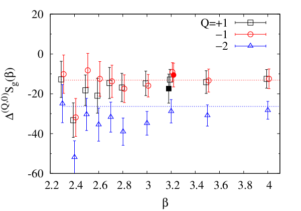
In quenched QCD, the dependence of is determined by
| (50) |
The results of with and are shown in Fig. 2, where it is seen that the data for and agree well within the statistical error as expected. Thus, the averaged value over and is used in the following analysis.
 |
 |
 |
 |
The horizontal dotted lines represent the action difference in the BPST instanton solutions, or in the high temperature limit, for and from top to bottom. The lattice data for are on top of the corresponding BPST line down to (or ) and suddenly decrease at . The similar behavior is observed for but the deviation from the corresponding BPST line starts at slightly larger , . The jump observed at may be associated with the phase transition. Studying the phase transition itself within this framework is interesting, but we focus on the high temperature region in this paper.
The large volume results are also shown in Fig. 2 (filled symbols). It is confirmed that the result are consistent with that from the smaller lattice. We omit the result on the larger lattice from the figure because of a large uncertainty.
In order to estimate using with or , we need to know . is empirically known 88 8 See the discussion around eq. (23).. We can estimate by looking at [see eq. (38)]. Figure 3 shows that is consistent with two over the whole range of we have studied, but the large statistical errors do not allow the precise determination except for the region of . It is seen that, when the mean value is relatively large, the error is also large. Thus, we assume in the following analysis.
The QCD beta function, , down to a low energy scale () is necessary in estimating eq. (50). We use the result of Ref. [34], in which the lattice spacing is expressed as a function of the lattice gauge coupling, , as
| (51) |
where denotes the string tension and
| , | (52) |
| (53) |
Using this expression, is numerically determined through
| (54) |
At the same time, the relationship between and is found to be
| (55) |
where and [34]. and are shown as a function of the lattice gauge coupling in Fig. 4.
 |
In the plot, we also show , which approaches to in the large limit.
Substituting the above results into eq. (50), is calculated as shown in Fig. 5, where the two solid curves represent the prediction of the DIGA (13) with and , respectively although they can not be distinguished at this axis scale.
 |
 |
The results with and are consistent with each other, which is expected from the observation in Fig. 3. These results are also consistent with the high temperature limit and the DIGA down to . Note that the results using the sector has the uncertainty smaller than those using by a factor , which indicates that once the has been fixed one can obtain very accurate result by performing a simulation at large .
One of the concerns in this approach is the finite volume effect since the physical volume becomes extremely small at large . Figure 5 shows that the lattice results well reproduce the high temperature limit at high temperature. From this observation, it is unlikely that the finite size effect significantly affects the lattice results, and it is natural to think that is the necessary condition for the finite volume effects to be under control. Indeed, the aspect ratio of our lattices is , and hence the above condition seems to be satisfied. Nevertheless, calculations with different lattice sizes are clearly useful to explicitly check the finite size effect and whether holds or not. However, since the uncertainty of the action value grows as , we need the statistics proportional to to keep the size of the uncertainty constant.
From the phenomenological point of view, for is important. In this range of , the statistical uncertainty is relatively large (typically for trajectories), which makes the axion abundance ambiguous. It is thus important to accumulate a large number of statistics. On the other hand, if behaves like a step function, our method should be able to detect such a behavior.
V summary and future prospects
The QCD topological susceptibility, , at high temperature provides an important input for the estimate of the axion abundance in the present universe. Existing methods to calculate on the lattice in the literature fail when . We proposed a novel lattice method to calculate the temperature dependence of the susceptibility, which is expected to work well especially in high temperature region where . To see how it works, we performed quenched simulations on the lattice, and found that the results of well agree with the DIGA prediction above . The simulation on a slightly larger lattice confirms that there is no unexpected large finite volume effect, although keeping the statistical error constant requires statistics proportional to . Thus, that error may be the main source of uncertainty in future serious works.
To predict the axion abundance, we still have to include dynamical quarks with the physical masses. In order for the method to work, the difference of the chiral condensate between two topological sectors has to be precisely determined, for which the dynamical overlap fermion seems to be preferred. Then, accumulating a large number of configurations requires large amount of resources. But, if behaves like a step function, a large number of statistics may not be necessary to detect such a behavior.
A possible way out is to generate configurations in large sectors, with which one can achieve an uncertainty smaller than that with by a factor of . Note that this requires the signal on [eq. (43)] at to be sufficiently precise to unambiguously identify the integer . Knowing for various is also useful to put the constraints on the dependence of in eq. (15), whose general form would be given by
| (56) |
with .
Acknowledgement
This work is in part based on Bridge++ code (http://bridge.kek.jp/Lattice-code/). This work is supported by JSPS KAKENHI Grant-in-Aid for Scientific Research (B) (No. 15H03669 [JF, RK, NY]) and MEXT KAKENHI Grant-in-Aid for Scientific Research on Innovative Areas (No. 25105011 [RK]), and also by the Large Scale Simulation Program No. 15/16-21 of High Energy Accelerator Research Organization (KEK).
Appendix A quark actions
The Wilson and overlap actions mentioned in the main text are described below. The Wilson quark action is given by
| (57) |
where
| (58) |
where is the link variable in the direction. The Hermitian Wilson Dirac operator appearing in eq. (49) is then given by
| (59) |
Note that, when using the Hermitian Wilson Dirac operator in the topology fixing term and the kernel of the overlap Dirac operator (see below), the mass has to be negative.
We adopt the fermionic definition based on the index theorem to estimate the topological charge for given configurations, which requires the number of zero modes of the overlap Dirac operator [35]. The overlap quark action and Dirac operator is given by
| (60) | |||||
| (61) | |||||
| (62) |
We calculated the low-lying eigenvalues of the Hermitian overlap Dirac operator, , and count the number of left- and right-handed zero modes. With the above definitions, it is straightforward to derive eqs. (33) and (34).
Appendix B the case
The relationship between expectation values in the vacuum and a fixed topological sector is derived in Refs. [36, 37, 38], where the results are written in the form of expansion (). From eq. (2.38) of Ref. [38], it is read that
where is defined as the coefficient of in the expansion,
| (64) |
especially . Note that is dynamical quantity and depends on . No assumption is made in deriving eq. () except for and , but in order for the expansion to be sensible, is required. It is interesting to see that eq. () is proportional to while the same quantity is to when [see, for example, eq. (39)].
Using eq. () and estimating , one can estimate the dependence of through eq. (25). Although can be directly estimated on the lattice as explained in the main text, we can further use the relationship between expectation values in the vacuum and a fixed topological sector [36, 37, 38] to proceed. From eq. (3.20) in Ref. [38], it follows that
| (65) |
where are defined as follows,
| (66) | |||||
| (67) | |||||
| (68) | |||||
| (69) |
is defined by
| (70) |
and . The expansion in eq. (65) is sensible if .
Applying the above expansions to the quenched case yields
| (71) | |||||
where
| (72) |
Appendix C hopping parameter expansion
We consider the temperature dependence of in the presence of flavors of heavy quarks (and no light quarks). In the following, we assume that the degenerate heavy mass is larger than the temperature, . By introducing the hopping parameter
| (73) |
the Wilson Dirac operator, eq. (58), can be rewritten as
Thus, when , we can expand in terms of .
If we take the Wilson fermion as the heavy quark action, the partition function and the expectation value of operator in a fixed topology sector can be written as
| (75) | |||||
| (76) |
respectively. Applying the hopping parameter expansion (HPE) to the heavy quarks, the determinant can be expanded as
| (77) | |||||
| (78) |
where denotes the real part of the Polyakov loop and we have used . Then, the expectation value, eq. (76), is given by
| (79) |
If consists of quark fields like , the HPE is further applied. Using
| (80) |
can be written as
| (81) | |||||
In summary,
| (82) | |||||
It turns out that, in the heavy quark region, the Polyakov loop plays an important role.
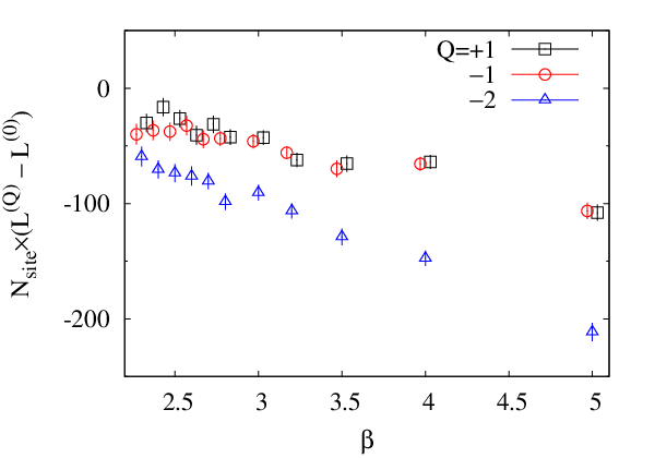
In Fig. 6, the difference of in different sectors is shown.
 |
 |
We define the following quantities,
| (83) | |||||
| (84) |
where we omit the term including the anomalous dimension of quark mass. Figure 7 shows the dependence of the above two quantities with .
 |
 |
 |
 |
 |
It turns out that the contribution of is much smaller than that of except for . Thus, omitting the term of the anomalous dimension does affect the final result by much.
is plotted in Fig. 8, which shows no clear dependence up to except at . At , the critical kappa is , thus the result at explores the relatively light quark mass region and may indicate a tendency that decreases towards the chiral limit, although the convergence of the HPE has to be checked.
 |
 |
 |
 |
 |
References
- [1] R. D. Peccei and H. R. Quinn, “CP Conservation in the Presence of Instantons,” Phys. Rev. Lett. 38, 1440 (1977).
- [2] R. D. Peccei and H. R. Quinn, “Constraints Imposed by CP Conservation in the Presence of Instantons,” Phys. Rev. D 16, 1791 (1977).
- [3] S. Weinberg, “A New Light Boson?,” Phys. Rev. Lett. 40, 223 (1978).
- [4] F. Wilczek, “Axions and Family Symmetry Breaking,” Phys. Rev. Lett. 49, 1549 (1982).
- [5] J. E. Kim, “Weak Interaction Singlet and Strong CP Invariance,” Phys. Rev. Lett. 43, 103 (1979).
- [6] M. A. Shifman, A. I. Vainshtein and V. I. Zakharov, “Can Confinement Ensure Natural CP Invariance of Strong Interactions?,” Nucl. Phys. B 166, 493 (1980).
- [7] M. Dine, W. Fischler and M. Srednicki, “A Simple Solution to the Strong CP Problem with a Harmless Axion,” Phys. Lett. B 104, 199 (1981).
- [8] A. R. Zhitnitsky, “On Possible Suppression of the Axion Hadron Interactions. (In Russian),” Sov. J. Nucl. Phys. 31, 260 (1980) [Yad. Fiz. 31, 497 (1980)].
- [9] J. Preskill, M. B. Wise and F. Wilczek, “Cosmology of the Invisible Axion,” Phys. Lett. B 120, 127 (1983).
- [10] L. F. Abbott and P. Sikivie, “A Cosmological Bound on the Invisible Axion,” Phys. Lett. B 120, 133 (1983).
- [11] M. Dine and W. Fischler, “The Not So Harmless Axion,” Phys. Lett. B 120, 137 (1983).
- [12] G. ’t Hooft, “Computation of the Quantum Effects Due to a Four-Dimensional Pseudoparticle,” Phys. Rev. D 14, 3432 (1976) [Phys. Rev. D 18, 2199 (1978)].
- [13] R. D. Pisarski and L. G. Yaffe, “The Density Of Instantons At Finite Temperature,” Phys. Lett. B 97, 110 (1980).
- [14] D. J. Gross, R. D. Pisarski and L. G. Yaffe, “QCD and Instantons at Finite Temperature,” Rev. Mod. Phys. 53, 43 (1981).
- [15] O. Wantz and E. P. S. Shellard, “Axion Cosmology Revisited,” Phys. Rev. D 82, 123508 (2010) [arXiv:0910.1066 [astro-ph.CO]].
- [16] S. Aoki, H. Fukaya and Y. Taniguchi, “Chiral symmetry restoration, eigenvalue density of Dirac operator and axial U(1) anomaly at finite temperature,” Phys. Rev. D 86 (2012) 114512 [arXiv:1209.2061 [hep-lat]].
- [17] T. Kanazawa and N. Yamamoto, “U (1) axial symmetry and Dirac spectra in QCD at high temperature,” JHEP 1601, 141 (2016) doi:10.1007/JHEP01(2016)141 [arXiv:1508.02416 [hep-th]].
- [18] R. Kitano and N. Yamada, “Topology in QCD and the axion abundance,” JHEP 1510, 136 (2015) [arXiv:1506.00370 [hep-ph]].
- [19] E. Berkowitz, M. I. Buchoff and E. Rinaldi, “Lattice QCD input for axion cosmology,” Phys. Rev. D 92, no. 3, 034507 (2015) [arXiv:1505.07455 [hep-ph]].
- [20] S. Borsanyi et al., “Axion cosmology, lattice QCD and the dilute instanton gas,” Phys. Lett. B 752, 175 (2016) [arXiv:1508.06917 [hep-lat]].
- [21] C. Bonati, M. D’Elia, M. Mariti, G. Martinelli, M. Mesiti, F. Negro, F. Sanfilippo and G. Villadoro, “Axion phenomenology and -dependence from lattice QCD,” arXiv:1512.06746 [hep-lat].
- [22] P. Petreczky, H. P. Schadler and S. Sharma, “The topological susceptibility in finite temperature QCD and axion cosmology,” arXiv:1606.03145 [hep-lat].
- [23] A. Laio, G. Martinelli and F. Sanfilippo, “Metadynamics Surfing on Topology Barriers: the CP(N-1) Case,” arXiv:1508.07270 [hep-lat].
- [24] A. A. Belavin, A. M. Polyakov, A. S. Schwartz and Y. S. Tyupkin, “Pseudoparticle Solutions of the Yang-Mills Equations,” Phys. Lett. B 59, 85 (1975). doi:10.1016/0370-2693(75)90163-X
- [25] C. W. Bernard, “Gauge Zero Modes, Instanton Determinants, and QCD Calculations,” Phys. Rev. D 19, 3013 (1979). doi:10.1103/PhysRevD.19.3013
- [26] M. Luscher, “Dimensional Regularization in the Presence of Large Background Fields,” Annals Phys. 142, 359 (1982). doi:10.1016/0003-4916(82)90076-8
- [27] R. D. Carlitz and D. B. Creamer, “Light Quarks and Instantons,” Annals Phys. 118, 429 (1979). doi:10.1016/0003-4916(79)90133-7
- [28] V. A. Novikov, M. A. Shifman, A. I. Vainshtein and V. I. Zakharov, “Calculations in External Fields in Quantum Chromodynamics. Technical Review,” Fortsch. Phys. 32, 585 (1984).
- [29] O. K. Kwon, C. k. Lee and H. Min, “Massive field contributions to the QCD vacuum tunneling amplitude,” Phys. Rev. D 62, 114022 (2000) doi:10.1103/PhysRevD.62.114022 [hep-ph/0008028].
- [30] G. V. Dunne, J. Hur, C. Lee and H. Min, “Calculation of QCD instanton determinant with arbitrary mass,” Phys. Rev. D 71, 085019 (2005) doi:10.1103/PhysRevD.71.085019 [hep-th/0502087].
- [31] B. J. Harrington and H. K. Shepard, “Periodic Euclidean Solutions and the Finite Temperature Yang-Mills Gas,” Phys. Rev. D 17, 2122 (1978). doi:10.1103/PhysRevD.17.2122
- [32] H. Fukaya et al. [JLQCD Collaboration], “Lattice gauge action suppressing near-zero modes of H(W)”, Phys. Rev. D 74, 094505 (2006) [hep-lat/0607020].
- [33] G. Cossu, S. Aoki, H. Fukaya, S. Hashimoto, T. Kaneko, H. Matsufuru and J. -I. Noaki, “Finite temperature study of the axial U(1) symmetry on the lattice with overlap fermion formulation”, Phys. Rev. D 87 (2013) 114514 [arXiv:1304.6145 [hep-lat]].
- [34] M. Okamoto et al. [CP-PACS Collaboration], “Equation of state for pure SU(3) gauge theory with renormalization group improved action”, Phys. Rev. D 60, 094510 (1999) [hep-lat/9905005].
- [35] H. Neuberger, “More about exactly massless quarks on the lattice,” Phys. Lett. B 427, 353 (1998) [hep-lat/9801031].
- [36] R. Brower, S. Chandrasekharan, J. W. Negele and U. J. Wiese, “QCD at fixed topology,” Phys. Lett. B 560, 64 (2003) doi:10.1016/S0370-2693(03)00369-1 [hep-lat/0302005].
- [37] S. Aoki, H. Fukaya, S. Hashimoto and T. Onogi, “Finite volume QCD at fixed topological charge,” Phys. Rev. D 76, 054508 (2007) doi:10.1103/PhysRevD.76.054508 [arXiv:0707.0396 [hep-lat]].
- [38] A. Dromard and M. Wagner, “Extracting hadron masses from fixed topology simulations,” Phys. Rev. D 90, no. 7, 074505 (2014) doi:10.1103/PhysRevD.90.074505 [arXiv:1404.0247 [hep-lat]].