Scalable Semi-supervised Learning with Graph-based Kernel Machine

Semi-supervised learning (SSL) aims at utilizing the intrinsic information carried in unlabeled data to enhance the generalization capacity of the learning algorithms. During the past decade, SSL has attracted significant attention and has found applicable in a variety of real-world problems including text categorization Joachims (1999), image retrieval Wang et al. (2003), bioinformatics Kasabov et al. (2005), natural language processing Goutte et al. (2002) to name a few. While obtaining pre-defined labels is a labor-intensive and time-consuming process Chapelle et al. (2008), it is well known that unlabeled data, when being used in conjunction with a small amount of labeled data, can bring a remarkable improvement in classification accuracy Joachims (1999).

A notable approach to semi-supervised learning paradigm is to employ spectral graph in order to represent the adjacent and distributive information carried in data. Graph-based methods are nonparametric, discriminative, and transductive in nature. Typical graph-based methods include min-cut Blum et al. (2004), harmonic function Zhu et al. (2003), graph random walk Azran (2007), spectral graph transducer Joachims (2003); Duong et al. (2015), and manifold regularization Belkin et al. (2006).

Inspired from the pioneering work of Joachims (1999), recent works have attempted to incorporate kernel methods such as Support Vector Machine (SVM) Cortes and Vapnik (1995) with the semi-supervised learning paradigm. The underlying idea is to solve the standard SVM problem while treating the unknown labels as optimization variables Chapelle et al. (2008). This leads to a non-convex optimization problem with a combinatorial explosion of label assignments. A wide spectrum of techniques have been proposed to solve this non-convex optimization problem, e.g., local combination search Joachims (1999), gradient descent Chapelle and Zien (2005), continuation techniques Chapelle et al. (2006), convex-concave procedures Collobert et al. (2006), deterministic annealing Sindhwani et al. (2006); Le et al. (2013); Nguyen et al. (2014), and semi-definite programming De Bie and Cristianini (2006). Although these works can somehow handle the combinatorial intractability, their common requirement of repeatedly retraining the model limits their applicability to real-world applications, hence lacking the ability to perform online learning for large-scale applications.

Conjoining the advantages of kernel method and the spectral graph theory, several existing works have tried to incorporate information carried in a spectral graph for building a better kernel function Kondor and Lafferty (2002); Chapelle et al. (2003); Smola and Kondor (2003). Basically, these methods employ the Laplacian matrix induced from the spectral graph to construct kernel functions which can capture the features of the ambient space. Manifold regularization framework Belkin et al. (2006) exploits the geometric information of the probability distribution that generates data and incorporates it as an additional regularization term. Two regularization terms are introduced to control the complexity of the classifier in the ambient space and the complexity induced from the geometric information of the distribution. However, the computational complexity for manifold regularization approach is cubic in the training size $n$ (i.e., $\textrm{O}\left(n^{3}\right)$). Hence other researches have been carried out to enhance the scalability of the manifold regularization framework Sindhwani and Niyogi (2005); Tsang and Kwok (2006); Melacci and Belkin (2011). Specifically, the work of Melacci and Belkin (2011) makes use of the preconditioned conjugate gradient to solve the optimization problem encountered in manifold regularization framework in the primal form, reducing the computational complexity from $\textrm{O}\left(n^{3}\right)$ to $\textrm{O}\left(n^{2}\right)$. However, this approach is not suitable for online learning setting since it actually solves the optimization problem in the first dual layer instead of the primal form. In addition, the LapSVM in primal approach Melacci and Belkin (2011) requires storing the entire Hessian matrix of size $n\times n$ in the memory, resulting in a memory complexity of $\text{O}(n^{2})$. Our evaluating experiments with LapSVM in primal further show that it always consumes a huge amount of memory in its execution (cf. Table 5).

Recently, stochastic gradient descent (SGD) methods Shalev-shwartz and Singer (2007); Kakade and Shalev-Shwartz (2008); Lacoste-Julien et al. (2012) have emerged as a promising framework to speed up the training process and enable the online learning paradigm. SGD possesses three key advantages: (1) it is fast; (2) it can be exploited to run in online mode; and (3) it is efficient in memory usage. In this paper, we leverage the strength from three bodies of theories, namely kernel method, spectral graph theory and stochastic gradient descent to propose a novel approach to semi-supervised learning, termed as Graph-based Semi-supervised Kernel Machine (GKM). Our GKM is applicable for a wide spectrum of loss functions (cf. Section 5) and smoothness functions $l_{p}\left(.\right)$ where $p\geq 1$ (cf. Eq. (4.1)). In addition, we note that the well-known Laplacian Support Vector Machine (LapSVM) Belkin et al. (2006); Melacci and Belkin (2011) is a special case of GKM(s) when using Hinge loss and the smoothness function $l_{2}\left(.\right)$. We then develop a new algorithm based on the SGD framework Lacoste-Julien et al. (2012) to directly solve the optimization problem of GKM in its primal form with the ideal convergence rate $\textrm{O}\left(\frac{1}{T}\right)$. At each iteration, a labeled instance and an edge in the spectral graph are randomly sampled. As the result, the computational cost at each iteration is very economic, hence making the proposed method efficient to deal with large-scale datasets while maintaining comparable predictive performance.

To summarize, our contributions in this paper are as follows:

• •

  We provide a novel view of jointly learning the kernel method with a spectral graph for semi-supervised learning. Our proposed GKM enables the combination of a wide spectrum of convex loss functions and smoothness functions.

• •

  We use the stochastic gradient descent (SGD) to solve directly GKM in its primal form. Hence, GKM has all advantageous properties of SGD-based methods including fast computation, memory efficiency, and online setting. To the best of our knowledge, the proposed GKM is the first kernelized semi-supervised learning method that can deal with the online learning context for large-scale application.

• •

  We provide a theoretical analysis to show that GKM has the ideal convergence rate $\text{O}\left(\frac{1}{T}\right)$ if the function is smooth and the loss function satisfies a proper condition. We then verify that this necessary condition holds for a wide class of loss functions including Hinge, smooth Hinge, and Logistic for classification task and L1, $\varepsilon$-insensitive for regression task (cf. Section 5).

• •

  The experimental results further confirm the ideal convergence rate $\text{O}\left(\frac{1}{T}\right)$ of GKM empirically and show that GKM is readily scalable for large-scale datasets. In particular, it offers a comparable classification accuracy whilst achieving a significant computational speed-up in comparison with the state-of-the-art baselines.

We review the works in semi-supervised learning paradigm that are closely related to ours. Graph-based semi-supervised learning is an active research topic under semi-supervised learning paradigm. At its crux, graph-based semi-supervised methods define a graph where the vertices are labeled and unlabeled data of the training set and edges (may be weighted) reflect the similarity of data. Most of graph-based methods can be interpreted as estimating the prediction function $f$ such that: it should predict the labeled data as accurate as possible; and it should be smooth on the graph.

In (Blum and Chawla, 2001; Blum et al., 2004), semi-supervised learning problem is viewed as graph mincut problem. In the binary case, positive labels act as sources and negative labels act as sinks. The objective is to find a minimum set of edges whose removal blocks all flow from the sources to the sinks. Another way to infer the labels of unlabeled data is to compute the marginal probability of the discrete Markov random field. In (Zhu and Ghahramani, 2002), Markov Chain Monte Carlo sampling technique is used to approximate this marginal probability. The work of (Getz et al., 2006) proposes to compute the marginal probabilities of the discrete Markov random field at any temperature with the Multi-canonical Monte Carlo method, which seems to be able to overcome the energy trap faced by the standard Metropolis or Swendsen - Wang method. The harmonic functions used in (Zhu et al., 2003) is regarded as a continuous relaxation of the discrete Markov random field. It does relaxation on the value of the prediction function and makes use of the quadratic loss with infinite weight so that the labeled data are clamped. The works of (Kondor and Lafferty, 2002; Chapelle et al., 2003; Smola and Kondor, 2003) utilize the Laplacian matrix induced from the spectral graph to form kernel functions which can capture the features of the ambient space.

Yet another successful approach in semi-supervised learning paradigm is the kernel-based approach. The kernel-based semi-supervised methods are primarily driven by the idea to solve a standard SVM problem while treating the unknown labels as optimization variables (Chapelle et al., 2008). This leads to a non-convex optimization problem with a combinatorial explosion of label assignments. Many methods have been proposed to solve this optimization problem, for example local combinatorial search (Joachims, 1999), gradient descent (Chapelle and Zien, 2005), continuation techniques (Chapelle et al., 2006), convex-concave procedures (Collobert et al., 2006), deterministic annealing (Sindhwani et al., 2006; Le et al., 2013; Nguyen et al., 2014), and semi-definite programming (De Bie and Cristianini, 2006). However, the requirement of retraining the whole dataset over and over preludes the applications of these kernel-based semi-supervised methods to the large-scale and streaming real-world datasets.

Some recent works on semi-supervised learning have primarily concentrated on the improvements of its safeness and classification accuracy. Li and Zhou (2015) assumes that the low-density separators can be diverse and an incorrect selection may result in a reduced performance and then proposes S4VM to use multiple low-density separators to approximate the ground-truth decision boundary. S4VM is shown to be safe and to achieve the maximal performance improvement under the low-density assumption of S3VM (Joachims, 1999). Wang et al. (2015) extends (Belkin et al., 2006; Wu et al., 2010) to propose semi-supervised discrimination-aware manifold regularization framework which considers the discrimination of all available instances in learning of manifold regularization. Tan et al. (2014) proposes using the $p$-norm as a regularization quantity in manifold regularization framework to perform the dimensionality reduction task in the context of semi-supervised learning.

The closest work to ours is the manifold regularization framework (Belkin et al., 2006) and its extensions (Sindhwani and Niyogi, 2005; Tsang and Kwok, 2006; Melacci and Belkin, 2011). However, the original work of manifold regularization (Belkin et al., 2006) requires to invert a matrix of size $n$ by $n$ which costs cubically and hence is not scalable. Addressing this issue, Tsang and Kwok (2006) scales up the manifold regularization framework by adding in an $\varepsilon$-insensitive loss into the energy function, i.e., replacing $\sum w_{ij}\left(f\left(x_{i}\right)-f\left(x_{j}\right)\right)^{2}$ by $\sum w_{ij}\left(\left|f\left(x_{i}\right)-f\left(x_{j}\right)\right|_{\varepsilon}\right)^{2}$, where $\left|z\right|_{\varepsilon}=\max\left\{\left|z\right|-\varepsilon,0\right\}$. The intuition is that most pairwise differences $\left|f\left(x_{i}\right)-f\left(x_{j}\right)\right|$ are very small. By ignoring the differences smaller than $\varepsilon$, the solution becomes sparser. LapSVM (in primal) (Melacci and Belkin, 2011) employs the preconditioned conjugate gradient to solve the optimization problem of manifold regularization in the primal form. This allows the computational complexity to be scaled up from $\textrm{O}\left(n^{3}\right)$ to $\textrm{O}\left(n^{2}\right)$. However, the optimization problem in (Melacci and Belkin, 2011) is indeed solved in the first dual layer rather than in the primal form. Furthermore, we empirically show that LapSVM in primal is expensive in terms of memory complexity (cf. Table 5).

Finally, the preliminary results of this work has been published in (Le et al., 2016) where it presents a special case of this work in which the combination of Hinge loss and the smoothness function $l_{1}\left(\cdot\right)$ is employed. In addition, our preliminary work (Le et al., 2016) guarantees only the convergence rate $\text{O}\left(\frac{\log\,T}{T}\right)$. In this work, we have substantially expanded (Le et al., 2016) and developed more powerful theory that guarantees the ideal convergence rate. We then further developed theory and analysis in order to enable the employment of a wide spectrum of loss and smoothness functions. Finally, we expanded significantly on the new technical contents, explanations as well as more extensive empirical studies.

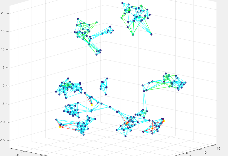
Our spectral graph is defined as a pair $\mathcal{G}=\left(\mathcal{V},\mathcal{E}\right)$ comprising a set $\mathcal{V}$ of vertices or nodes or points together with a set $\mathcal{E}$ of edges or arcs or lines, which are 2-element subsets of $V$ (i.e. an edge is associated with two vertices, and that association takes the form of the unordered pair comprising those two vertices). In the context of semi-supervised learning, we are given a training set $X=X_{l}\cup X_{u}$ where $X_{l}=\left\{\left(x_{i},y_{i}\right)\right\}_{i=1}^{l}$ is labeled data and $X_{u}=\left\{x_{i}\right\}_{i=l+1}^{l+u}$ is unlabeled data. We construct the vertex set $\mathcal{V}$ includes all labeled and unlabeled instances (i.e., $\mathcal{V}=\left\{x_{i}\right\}_{i=1}^{l+u}$). An edge $e_{ij}=\overline{x_{i}x_{j}}\in\mathcal{E}$ between two vertices $x_{i},\,x_{j}$ represents the similarity of the two instances. Let $\mu_{ij}$ be the weight associated with edge $e_{ij}$. The underlying principle is to enforce that if $\mu_{ij}$ is large, then $y_{i}$ and $y_{j}$ are expected to receive the same label. The set of edges $\mathcal{G}$ and its weighs can be built using the following ways (Zhu et al., 2009; Le et al., 2016):

• •

  Fully connected graph: every pair of vertices $x_{i}$, $x_{j}$ is connected by an edge. The edge weight decreases when the distance $||x_{i}-x_{j}||$ increases. The Gaussian kernel function widely used is given by $\mu_{ij}=\text{exp}\left(-\|x_{i}-x_{j}\|^{2}/\left(2\sigma_{s}^{2}\right)\right)$ where $\sigma_{s}$ controls how quickly the weight decreases.

• •

  $k$-NN: each vertex $x_{i}$ determines its $k$ nearest neighbors ($k$-NN) and makes an edge with each of its $k$-NN. The Gaussian kernel weight function can be used for the edge weight. Empirically, $k$-NN graphs with small $k$ tend to perform well.

• •

  $\varepsilon$-NN: we connect $x_{i}$ and $x_{j}$ if $\left\|x_{i}-x_{j}\right\|\leq\varepsilon$. Again the Gaussian kernel weight function can be used to weight the connected edges. In practice, $\varepsilon$-NN graphs are easier to construct than $k$-NN graphs.

When constructing a graph, we avoid connecting the edge of two labeled instances since we do not need to propagate the label between them. Figure 1 illustrates an example of graph constructed on 3D dataset using $k$-NN with $k=5$.

After constructing a graph, we formulate a semi-supervised learning problem as assigning labels to the unlabeled vertices via label propagation. We propagate the labels from the labeled vertices to the unlabeled ones by encouraging $y_{i}$ to have the same label as $y_{j}$ if the weight $\mu_{ij}$ is large and vice versa. To do so, we learn a mapping function $f:\,\mathfrak{\mathcal{X}}\rightarrow\mathcal{Y}$ where $\mathcal{X}$ and $\mathcal{Y}$ are the domains of data and label such that

• •

  $f\left(x_{i}\right)$ is as closest to its label $y_{i}$ as possible for all labeled instances $x_{i}\,\left(1\leq i\leq l\right)$.

• •

  $f$ should be smooth on the graph $\mathcal{G}$, i.e., if $x_{i}$ is very close to $x_{j}$ (i.e., $\mu_{ij}$ is large), the discrepancy between $f_{i}$ and $f_{j}$ (i.e., $|f_{i}-f_{j}|$) is small.

Therefore, we obtain the optimization problem (Zhu et al., 2009; Le et al., 2016) as

In this section, we present our proposed Graph-based Semi-supervised Kernel Machine (GKM). We begin with formulating the optimization problem for GKM, followed by the derivation of an SGD-based solution. Finally, we present the convergence analysis for our proposed method. The convergence analysis shows that our proposed method gains the ideal convergence rate $\text{O}\left(\frac{1}{T}\right)$ for combinations of the typical loss functions (cf. Section 5) and the smoothness functions with $p\geq 1$.

In this section, we present the suitability of five loss and kernel functions that can be used for GKM including hinge, smooth hinge, logistic, L1, and $\epsilon$-insensitive. We verify that most of the well-known loss functions satisfy the necessary condition: $\left\|\nabla_{\mathbf{w}}l\left(\mathbf{w};x,y\right)\right\|\leq A$ for an appropriate positive number $A$. By allowing multiple choices of loss functions, we enable broader applicability of the proposed GKM for real-world applications while the work of (Le et al., 2016) is restricted to a Hinge loss function.

• •

  Hinge loss: $l\left(\mathbf{w};x,y\right)=\max\left\{0,1-y\mathbf{w}^{\mathsf{T}}\Phi\left(x\right)\right\}$,

  $\displaystyle\nabla_{\mathbf{w}}l\left(\mathbf{w};x,y\right)$

  $\displaystyle=-\mathbb{I}_{\left\{y\mathbf{w}^{\mathsf{T}}\Phi\left(x\right)\leq 1\right\}}y\Phi\left(x\right)$

  Therefore, by choosing $A=R$ we have $\left\|\nabla_{\mathbf{w}}l\left(\mathbf{w};x,y\right)\right\|\leq\left\|\Phi\left(x\right)\right\|\leq R=A$.

• •

  Smooth Hinge loss (Shalev-Shwartz and Zhang, 2013):

  	$\displaystyle l\left(\mathbf{w};x,y\right)$	$\displaystyle=\begin{cases}0&\text{if}\,\,yo>1\\ 1-y\mathbf{w}^{\top}\Phi\left(x\right)-\frac{\tau}{2}&\text{if}\,\,yo<1-\tau\\ \frac{1}{2\tau}\left(1-yo\right)^{2}&\text{otherwise}\end{cases}$
  	$\displaystyle\nabla_{\mathbf{w}}l\left(\mathbf{w};x,y\right)$	$\displaystyle=-\mathbb{I}_{\left\{yo<1-\tau\right\}}y\Phi\left(x\right)+\tau^{-1}\mathbb{I}_{1-\tau\leq yo\leq 1}\left(yo-1\right)y\Phi\left(x\right)$

  where $o=\mathbf{w}^{\top}\Phi\left(x\right)$. Therefore, by choosing $A=R$ we have

  	$\displaystyle\left\|\nabla_{\mathbf{w}}l\left(\mathbf{w};x,y\right)\right\|$	$\displaystyle=R\left|\tau^{-1}\mathbb{I}_{1-\tau\leq yo\leq 1}\left(yo-1\right)\right|+R\mathbb{I}_{\left\{yo<1-\tau\right\}}$
  		$\displaystyle\leq\mathbb{I}_{\left\{yo<1-\tau\right\}}R+\tau^{-1}\tau\mathbb{I}_{1-\tau\leq yo\leq 1}R\leq R=A$

• •

  Logistic loss: $l\left(\mathbf{w};x,y\right)=\log\left(1+\exp\left(-y\mathbf{w}^{\mathsf{T}}\Phi\left(x\right)\right)\right)$,

  $\displaystyle\nabla_{\mathbf{w}}l\left(\mathbf{w};x,y\right)$

  $\displaystyle=\frac{-y\exp\left(-y\mathbf{w}^{\mathsf{T}}\Phi\left(x\right)\right)\Phi\left(x\right)}{\exp\left(-y\mathbf{w}^{\mathsf{T}}\Phi\left(x\right)\right)+1}$

  By choosing $A=R$ we have $\left\|\nabla_{\mathbf{w}}l\left(\mathbf{w};x,y\right)\right\|<\left\|\Phi\left(x\right)\right\|\leq R=A$.

• •

  L1 loss: $l\left(\mathbf{w};x,y\right)=|y-\mathbf{w}^{\mathsf{T}}\Phi\left(x\right)|$, $\nabla_{\mathbf{w}}l\left(\mathbf{w};x,y\right)=\text{sign}\left(\mathbf{w}^{\mathsf{T}}\Phi\left(x\right)-y\right)\Phi\left(x\right)$. By choosing $A=R$ we have $\left\|\nabla_{\mathbf{w}}l\left(\mathbf{w};x,y\right)\right\|\leq\left\|\Phi\left(x\right)\right\|\leq R=A$.

• •

  $\varepsilon$-insensitive loss: let denote $o=\mathbf{w}^{\mathsf{T}}\Phi\left(x\right)|$, $l\left(\mathbf{w};x,y\right)=\max\left\{0,|y-\mathbf{w}^{\mathsf{T}}\Phi\left(x\right)|-\varepsilon\right\}$,

  $\displaystyle\nabla_{\mathbf{w}}l\left(\mathbf{w};x,y\right)$

  $\displaystyle=\mathbb{I}_{\left\{|y-o>\varepsilon\right\}}\text{sign}\left(o-y\right)\Phi\left(x\right)$

  By choosing $A=R$ we have $\left\|\nabla_{\mathbf{w}}l\left(\mathbf{w};x,y\right)\right\|\leq\left\|\Phi\left(x\right)\right\|\leq R=A$.

Here, $\mathbb{I}_{S}$ is the indicator function which is equal to $1$ if the statement $S$ is true and $0$ if otherwise. It can be observed that the positive constant $A$ coincides the radius $R$ (i.e., $A=R$) for the aforementioned loss functions. To allow the ability to flexibly control the minimal sphere that encloses all $\Phi\left(x\right)$(s), we propose to use the squared exponential (SE) kernel function $k\left(x,x^{\prime}\right)=\sigma_{f}^{2}\text{exp}\left(-\left\|x-x^{\prime}\right\|^{2}/\left(2\sigma_{l}^{2}\right)\right)$ where $\sigma_{l}$ is the length-scale and $\sigma_{f}$ is the output variance parameter. Using SE kernel, we have the following equality $\left\|\Phi\left(x\right)\right\|=K\left(x,x\right)^{1/2}=\sigma_{f}\leq R$. Recall that if $p=2$ or $p>2$, Algorithm 1 converges to the optimal solution with the ideal convergence rate $\text{O}\left(\frac{1}{T}\right)$ under specific conditions. In particular, with $p=2$ the corresponding condition is $a<1$ and with $p>2$ the corresponding condition is $ab^{p-2}\leq\frac{\left(p-2\right)^{p-2}}{\left(p-1\right)^{p-1}}$ where $a=C^{\prime}\left(2R\right)^{p}p$ and $b=CA$. Using the SE kernel, we can adjust the output variance parameter $\sigma_{f}$ to make the convergent condition valid. More specifically, we consider two cases:

• •

  $p=2$: we have $a<1\rightarrow C^{\prime}\left(2R\right)^{p}p<1\rightarrow R<0.5\left(pC^{\prime}\right)^{-1/p}$. We can simply choose $\sigma_{f}$ with a very small number $\rho>0$

  $\displaystyle\sigma_{f}$

  $\displaystyle=R=0.5\left(pC^{\prime}\right)^{-1/p}-\rho=0.5\left(2C^{\prime}\right)^{-1/2}-\rho$

• •

  $p>2$: we have $ab^{p-2}\leq\left(p-2\right)^{p-2}\left(p-1\right)^{1-p}$ and then

  	$\displaystyle C^{\prime}\left(2R\right)^{p}p\left(CA\right)^{p-2}$	$\displaystyle\leq\left(p-2\right)^{p-2}\left(p-1\right)^{1-p}$
  	$\displaystyle R$	$\displaystyle\leq\left(\frac{\left(p-2\right)^{p-2}}{2^{p}C^{p-2}C^{\prime}p\left(p-1\right)^{p-1}}\right)^{\frac{1}{2p-2}}$

  We can simply choose $\sigma_{f}=R=\left(\frac{\left(p-2\right)^{p-2}}{2^{p}C^{p-2}C^{\prime}p\left(p-1\right)^{p-1}}\right)^{\frac{1}{2p-2}}$.

We can control the second trade-off parameter $C^{\prime}$ to ensure the ideal convergence rate $\text{O}\left(\frac{1}{T}\right)$ with $p\geq 2$. More specifically, we also consider two cases:

• •

  $p=2$: we have $a<1\rightarrow C^{\prime}<\left(2R\right)^{-p}p^{-1}=0.125$.

• •

  $p>2$: we have $ab^{p-2}\leq\left(p-2\right)^{p-2}\left(p-1\right)^{1-p}$ and thus

  $\displaystyle C^{\prime}$

  $\displaystyle\leq\frac{\left(p-2\right)^{p-2}}{2^{p}C^{p-2}p\left(p-1\right)^{p-1}}$

  (5)

We conduct the extensive experiments to investigate the influence of the model parameters and other factors to the model behavior and to compare our proposed GKM with the state-of-the-art baselines on the benchmark datasets. In particular, we design three kinds of experiments to analyze the influence of factors (e.g., the loss function, the smoothness function, and the percentage of unlabeled portion) to the model behavior. In the first experiment (cf. Section 6.1.1), we empirically demonstrate the theoretical convergence rate $\text{O}\left(\frac{1}{T}\right)$ for all combinations of loss function (Hinge and Logistic) and smoothness function ($p=1,2,3$) and also investigate how the number of iterations affects the classification accuracy. In the second experiment (cf. Section 6.1.2), we study the influence of the loss function and the smoothness function to the predictive performance and the training time when the percentage of unlabeled portion is either $80\%$ or $90\%$. In the third experiment (cf. Section 6.1.3), we examine the proposed method under the semi-supervised setting where the proportion of unlabeled data is varied from $50\%$ to $90\%$. Finally, we compare our proposed GKM with the state-of-the-art baselines on the benchmark datasets.

References

- Azran [2007] A. Azran. The rendezvous algorithm: Multiclass semi-supervised learning with markov random walks. In Proceedings of the 24th International Conference on Machine Learning, ICML ’07, pages 49–56, 2007.
- Belkin et al. [2006] M. Belkin, P. Niyogi, and V. Sindhwani. Manifold regularization: A geometric framework for learning from labeled and unlabeled examples. J. Mach. Learn. Res., 7:2399–2434, December 2006.
- Blum and Chawla [2001] A. Blum and S. Chawla. Learning from labeled and unlabeled data using graph mincuts. In Proceedings of the Eighteenth International Conference on Machine Learning, ICML ’01, pages 19–26, 2001.
- Blum et al. [2004] A. Blum, J. D. Lafferty, M. R. Rwebangira, and R. Reddy. Semi-supervised learning using randomized mincuts. In ICML, volume 69, 2004.
- Chang and Lin [2011] C.-C. Chang and C.-J. Lin. Libsvm: A library for support vector machines. ACM Trans. Intell. Syst. Technol., 2(3):27:1–27:27, May 2011. ISSN 2157-6904.
- Chapelle and Zien [2005] O. Chapelle and A. Zien. Semi-supervised classification by low density separation, 2005.
- Chapelle et al. [2003] O. Chapelle, J. Weston, and B. Schölkopf. Cluster kernels for semi-supervised learning. In Advances in Neural Information Processing Systems 15, pages 601–608. MIT Press, 2003.
- Chapelle et al. [2006] O. Chapelle, M. Chi, and A. Zien. A continuation method for semi-supervised svms. In Proceedings of the 23rd international conference on Machine learning, pages 185–192, 2006.
- Chapelle et al. [2008] O. Chapelle, V. Sindhwani, and S.S. Keerthi. Optimization techniques for semi-supervised support vector machines. Journal of Machine Learning Research, 9:203–233, June 2008.
- Collobert et al. [2006] R. Collobert, F. Sinz, J. Weston, L. Bottou, and T. Joachims. Large scale transductive svms. Journal of Machine Learning Research, 2006.
- Cortes and Vapnik [1995] C. Cortes and V. Vapnik. Support-vector networks. In Machine Learning, pages 273–297, 1995.
- De Bie and Cristianini [2006] T. De Bie and N. Cristianini. Semi-supervised learning using semi-definite programming. In Semi-supervised Learning, Cambridge, MA, 2006.
- Duong et al. [2015] P. Duong, V. Nguyen, M. Dinh, T. Le, D. Tran, and W. Ma. Graph-based semi-supervised support vector data description for novelty detection. In 2015 International Joint Conference on Neural Networks (IJCNN), pages 1–6, July 2015.
- Getz et al. [2006] G. Getz, N. Shental, and E. Domany. Semi-supervised learning – a statistical physics approach. CoRR, 2006.
- Goutte et al. [2002] C. Goutte, H. Déjean, E. Gaussier, N. Cancedda, and J-M Renders. Combining labelled and unlabelled data: A case study on fisher kernels and transductive inference for biological entity recognition. In Proceedings of the 6th Conference on Natural Language Learning - Volume 20, COLING-02, pages 1–7, 2002.
- Joachims [1999] T. Joachims. Transductive inference for text classification using support vector machines. In International Conference on Machine Learning (ICML), pages 200–209, 1999.
- Joachims [2003] T. Joachims. Transductive learning via spectral graph partitioning. In In ICML, pages 290–297, 2003.
- Kakade and Shalev-Shwartz [2008] S. Kakade and Shalev-Shwartz. Mind the duality gap: Logarithmic regret algorithms for online optimization. In NIPS, 2008.
- Kasabov et al. [2005] N. Kasabov, D. Zhang, and P.S. Pang. Incremental learning in autonomous systems: evolving connectionist systems for on-line image and speech recognition. In Advanced Robotics and its Social Impacts, 2005. IEEE Workshop on, pages 120 – 125, june 2005.
- Kondor and Lafferty [2002] R. I. Kondor and J. D. Lafferty. Diffusion kernels on graphs and other discrete input spaces. pages 315–322. Morgan Kaufmann Publishers Inc., 2002. ISBN 1-55860-873-7.
- Lacoste-Julien et al. [2012] S. Lacoste-Julien, M. W. Schmidt, and F. Bach. A simpler approach to obtaining an o(1/t) convergence rate for the projected stochastic subgradient method. CoRR, 2012.
- Le et al. [2013] T. Le, D. Tran, T. Tran, K. Nguyen, and W. Ma. Fuzzy entropy semi-supervised support vector data description. In International Joint Conference on Neural Networks (IJCNN), pages 1–5, Aug 2013.
- Le et al. [2016] Trung Le, Phuong Duong, Mi Dinh, Tu Dinh Nguyen, Vu Nguyen, and Dinh Phung. Budgeted semi-supervised support vector machine. In The 32th Conference on Uncertainty in Artificial Intelligence, pages 377–386. AUAI Press, 2016.
- Li and Zhou [2015] Y-F. Li and Z-H. Zhou. Towards making unlabeled data never hurt. Pattern Analysis and Machine Intelligence, IEEE Transactions on, 37(1):175–188, Jan 2015.
- Melacci and Belkin [2011] S. Melacci and M. Belkin. Laplacian support vector machines trained in the primal. J. Mach. Learn. Res., 12:1149–1184, July 2011.
- Nguyen et al. [2014] V. Nguyen, T. Le, T. Pham, M. Dinh, and T. H. Le. Kernel-based semi-supervised learning for novelty detection. In International Joint Conference on Neural Networks (IJCNN), pages 4129–4136, July 2014.
- Shalev-shwartz and Singer [2007] S. Shalev-shwartz and Y. Singer. Logarithmic regret algorithms for strongly convex repeated games. In The Hebrew University, 2007.
- Shalev-Shwartz and Zhang [2013] S. Shalev-Shwartz and T. Zhang. Stochastic dual coordinate ascent methods for regularized loss. Journal of Machine Learning Research, 14(1):567–599, 2013.
- Sindhwani and Niyogi [2005] V. Sindhwani and P. Niyogi. Linear manifold regularization for large scale semi-supervised learning. In Proc. of the 22nd ICML Workshop on Learning with Partially Classified Training Data, 2005.
- Sindhwani et al. [2006] V. Sindhwani, S.S. Keerthi, and O. Chapelle. Deterministic annealing for semi-supervised kernel machines. In Proceedings of the 23rd international conference on Machine learning, ICML ’06, pages 841–848, 2006.
- Smola and Kondor [2003] A. J. Smola and I. R. Kondor. Kernels and regularization on graphs. In Proceedings of the Annual Conference on Computational Learning Theory, 2003.
- Tan et al. [2014] J. Tan, L. Zhen, N. Deng, and Z. Zhang. Laplacian p-norm proximal support vector machine for semi-supervised classification. Neurocomputing, 144:151–158, 2014.
- Tsang and Kwok [2006] I. W. Tsang and J. T. Kwok. Large-scale sparsified manifold regularization. pages 1401–1408. MIT Press, 2006. ISBN 0-262-19568-2.
- Wang et al. [2003] L. Wang, K. L. Chan, and Z. Zhang. Bootstrapping svm active learning by incorporating unlabelled images for image retrieval. pages 629–634. IEEE Computer Society, 2003.
- Wang et al. [2015] Y. Wang, S. Chen, H. Xue, and Z. Fu. Semi-supervised classification learning by discrimination-aware manifold regularization. Neurocomputing, 147:299–306, 2015.
- Wu et al. [2010] F. Wu, W. Wang, Y. Yang, Y. Zhuang, and F. Nie. Classification by semi-supervised discriminative regularization. Neurocomputing, 73:1641 – 1651, 2010. ISSN 0925-2312.
- Zhu and Ghahramani [2002] X. Zhu and Z. Ghahramani. Towards semi-supervised classification with markov random fields, 2002.
- Zhu et al. [2003] X. Zhu, Z. Ghahramani, and J. D. Lafferty. Semi-supervised learning using gaussian fields and harmonic functions. In IN ICML, pages 912–919, 2003.
- Zhu et al. [2009] X. Zhu, A. B. Goldberg, R. Brachman, and T. Dietterich. Introduction to Semi-Supervised Learning. Morgan and Claypool Publishers, 2009. ISBN 1598295470, 9781598295474.