Systematic parameter inference in stochastic mesoscopic modeling
Abstract
We propose a method to efficiently determine the optimal coarse-grained force field in mesoscopic stochastic simulations of Newtonian fluid and polymer melt systems modeled by dissipative particle dynamics (DPD) and energy conserving dissipative particle dynamics (eDPD). The response surfaces of various target properties (viscosity, diffusivity, pressure, etc.) with respect to model parameters are constructed based on the generalized polynomial chaos (gPC) expansion using simulation results on sampling points (e.g., individual parameter sets). To alleviate the computational cost to evaluate the target properties, we employ the compressive sensing method to compute the coefficients of the dominant gPC terms given the prior knowledge that the coefficients are “sparse”. The proposed method shows comparable accuracy with the standard probabilistic collocation method (PCM) while it imposes a much weaker restriction on the number of the simulation samples especially for systems with high dimensional parametric space. Fully access to the response surfaces within the confidence range enables us to infer the optimal force parameters given the desirable values of target properties at the macroscopic scale. Moreover, it enables us to investigate the intrinsic relationship between the model parameters, identify possible degeneracies in the parameter space, and optimize the model by eliminating model redundancies. The proposed method provides an efficient alternative approach for constructing mesoscopic models by inferring model parameters to recover target properties of the physics systems (e.g., from experimental measurements), where those force field parameters and formulation cannot be derived from the microscopic level in a straight forward way.
Keywords:
Coarse-grained force field, dissipative particle dynamics, energy conserving dissipative particle dynamics, compressive sensing, generalized polynomial chaos, model reduction, high dimensionality1 Introduction
It is well known that many of the macroscopic properties observed in soft matter systems, such as liquid crystals, polymers, and colloids are natural consequences of the physical processes at the microscopic level. Accurate modeling of the corresponding processes enables us to successfully predict the properties of these material systems as well as, in turn, calibrate the parameters of the models. Molecular dynamics (MD) simulation, in conjunction with optimized force fields, has been successfully applied to study various physical systems [1, 2]. However, due to the explicit modeling of individual atomistic particles, the MD simulation method is limited and cannot reach the spatial and temporal scales relevant to the collective motion we are interested in, i.e., at the mesoscale.
To overcome this limitation, an alternative approach is to coarse grain (CG) the system by representing several atomistic particles as a single virtual particle. The essential idea is to eliminate the fast modes and corresponding degrees of freedom (DOF) while only keeping those DOFs relevant to the scale of our interest, represented as the CG particles. The static properties of the CG system are closely related to the governing force field, which have been studied extensively [3, 4, 5, 6, 7, 8, 9]. Espanõl [3] modeled the DPD particles by grouping several Lennard Jones (LJ) particles into clusters, and derived the conservative force field from the radial distribution function of the clusters. Bolhuis et al. [5] mapped the semi-dilute polymer solution onto soft particles via an effective pairwise potential. Kremer et al. [8] and Fukunaga et al. [9] extracted the effective force field for complex polymers from the distribution functions of the bond length, bending angle and torsion angle. By carefully choosing the CG sites (“super atoms”) and tuning the CG force field parameters, these CG models can reproduce the specified structural properties of the atomistic systems.
However, currently there are still two open questions for constructing the CG model and force field. First, most of the CG force fields are constructed by targeting certain static properties (e.g., the pair and angle distribution functions) of the atomistic system, while the constructed CG force fields show limitation if we consider other static properties (e.g., the equation of state) [10, 11]. In particular, how to construct a CG model with a thermodynamically consistent force field is still an open question. Moreover, the CG force fields are insufficient to reproduce the dynamic properties of the atomistic system. Instead, two additional (dissipative and random) force terms should be introduced to compensate for the eliminated atomistic DOFs during the CG procedure [12]. This is represented by the force terms in mesoscopic simulation methods such as dissipative particle dynamics (DPD) [13, 14] and its variations, e.g., energy-conserving dissipative particle dynamics (eDPD) [15, 16]. Computing the dissipative and random force terms directly from the atomistic systems is a non-trivial task. Eriksson et al. [17] estimated the dissipative force term by the force covariance function, whereas Lei et al. [11], Hijón et al. [18], Izvekov et al. [19] and Li et al. [20] computed the dissipative force term using the Mori-Zwanzig formulation [21, 22]. While the computed dissipative force terms successfully reproduce the dynamic properties in the dilute and semi-dilute regime, the force terms show limitation in reproducing the dynamic properties for highly correlated systems. Currently, it is still unclear how to determine the optimized CG force terms with correct dynamic properties at high density regime.
To circumvent those difficulties discussed above, we study the CG systems by considering an alternative question: if we are only interested in some particular properties (e.g., target properties) related to the physical system, how do we choose the optimal CG modeling parameters within certain confidence range? That is, how to calibrate the CG modeling parameters for a specific set of target properties observed at the macroscopic scale? We emphasize that the inferred parameters may not correspond to the values in mesoscopic models directly constructed from the microscopic systems in ab initio way. However, these parameters should be sufficient to recover the target properties we are interested in if the CG model is constructed appropriately. In this sense, this study also enables us to validate the proposed CG model as well as to analyze the sensitivity of the macroscopic quantities on individual modeling parameters.
In this work, we aim to investigate the static and dynamic properties of mesoscopic systems governed by the DPD/eDPD force field within a high dimensional random parameter space. In particular, we study the dynamic properties of two mesoscopic systems: a non-Newtonian polymer melt system governed by DPD force field within a 6-dimensional parameter space; and a non-isothermal model for liquid water at different temperatures governed by eDPD force field within a 4-dimensional parameter space. In order to calibrate the parameters in mesoscopic systems, we employ the Bayesian framework:
where are parameters to infer, are target properties, is the posterior distribution, is the likelihood function, and is the prior distribution. The selection of parameters relies on the posterior distribution , which is usually obtained by the Markov Chain Monte Carlo (MCMC) method [23, 24] or its variants. However, the MCMC method usually requires evaluating the likelihood function thousands of times, which in turn requires running the costly DPD simulation thousands of times. This requirement is prohibitive for complex systems, hence an accurate and fast surrogate model (which approximates the response surface) is necessary. In this work, we employ generalized polynomial chaos (gPC) [25, 26] to build the surrogate model for DPD systems in the form of a linear combination of a set of special basis functions defined in the parameter space. This idea has been used in solving inverse problems (e.g., [27, 28]) and MD modeling of water systems (e.g., [29, 30]). This gPC surrogate model facilitates the implementation of MCMC and dramatically accelerates the evaluation of the likelihood function , hence enabling us to infer the parameters efficiently.
The construction of surrogate models can be achieved by functional representations employed in uncertainty quantification (UQ), e.g., (adaptive) sparse grid method [31, 32, 33, 34, 35] or (adaptive) ANOVA method [36, 37, 38, 39]. All these methods are categorized as probabilistic collocation methods (PCM) as they provide smart strategies to select sampling points and weights. In recent years, efforts have been made to propose a non-adaptive but simple and accurate method for high dimensional problems [40, 41, 42, 43, 44, 45] when the system is sparse, which within the UQ framework means that only a small portion of the gPC coefficients has relatively large values while the others are close to zero. This idea stems from the compressive sensing field [46, 47, 48, 49]. More precisely, if we know a priori that the vector of gPC coefficients is sparse, we can employ compressive sensing techniques to “recover" these coefficients accurately using only a few (deterministic) simulation data. This method can be considered as post processing of the sampling method, e.g., Monte Carlo method or PCM method, hence it is flexible as we can always incorporate new available data and obtain better estimates. This method has an advantage over many popular methods, e.g., the standard sparse grid method, which is popular in UQ studies today, as it requires a fixed number of additional simulations to reach the next accuracy level. This requirement is prohibitive in practice when the dimension of the problem is high. Even with the adaptive method, the selection of adaptivity criteria can be constrained by the limitation of computational resources. Moreover, in MD and DPD simulations, due to the existence of the thermal noise, it is difficult to obtain a highly accurate gPC surrogate model. In other words, even if we can afford running simulations with a high order PCM method, we may not be able to reduce the error of the surrogate model. This is different from research on UQ in solving stochastic PDEs, where high accuracy can be expected with high order methods. Therefore, it is more helpful to adopt a method which can efficiently construct the gPC expansion with small errors (ideally close to the thermal noise level).
After obtaining a good surrogate model of the response surface of the target property, we employ the Bayesian inference to explore suitable model parameters in DPD. For material design problems, given the desirable target properties , we can firstly build a DPD model with empirical (commonly used) constants. Then, we parametrize these constants to obtain a parameter set . Next, we run the DPD simulation with different sets of values to obtain samples of target properties and build the gPC approximation (surrogate model) of target properties depending on via compressive sensing. Finally, we implement the Bayesian inference based on and the gPC expansion to infer the suitable for the DPD model. The above procedure can be repeated until the DPD model reaches the required accuracy by increasing the accuracy of the surrogate model or by modifying the range of the parameters. Figure 1 provides an overview of the entire procedure of inferring the parameters in the DPD model via gPC expansion and compressive sensing. The difference between and can be measured by the summation of relative error of each target property.
This paper is organized as follows. Section 2 is devoted to a brief introduction of the mesoscopic simulation method and models considered in the present study, i.e., the non-Newtonian polymer melt model based on dissipative particle dynamics (DPD) and the non-isothermal liquid water model based on the /energy-conserving dissipative particle dynamics (eDPD). In Section 3, we introduce the compressive sensing method and its application in the gPC coefficient computation. In Section 4, we construct the gPC expansions of various target properties over the parameter space for both the polymer melt and the liquid water systems. Using the gPC expansion as the surrogate model, we estimate the optimal force parameters and eliminate possible model redundancies with the prescribed value of the target properties via Bayesian inference. In Section 5, we summarize our work and briefly discuss future directions.
2 Simulation method and physical model
2.1 Dissipative Particle Dynamics
Dissipative Particle Dynamics (DPD) [13, 50] is a particle based mesoscopic simulation method. Each DPD particle represents a coarse-grained virtual cluster of multiple atomistic particles [11]. In standard DPD formulation [13], the motion of each particle is governed by
| (2.1) |
where , , are the position, velocity, and mass of the particle , and , , are the total conservative, dissipative and random forces acting on the particle , respectively. Under the assumption of pairwise interactions the DPD forces can be decomposed into pair interactions with the surrounding particles by
| (2.2) | ||||
where , , , and . is the cut-off radius beyond which all interactions vanish. The coefficients , and represent the strength of the conservative, dissipative and random force, respectively. The dissipative and random force terms are coupled with the system temperature by the fluctuation-dissipation theorem [14] as . Here, are independent identically distributed (i.i.d.) Gaussian random variables with zero mean and unit variance. The weight functions and are defined by
| (2.3) |
where is a parameter that determines the extent of dissipative and random force envelopes.
While this method was initially proposed [13] to simulate the complex hydrodynamic processes of isothermal fluid systems, the particle based feature enables us to easily incorporate additional physical models and extend its application to various soft matter and complex fluid systems, such as polymer and DNA suspensions [51, 52, 53], platelet aggregation [54], microgel [55], colloid suspension [56], droplet wetting [57] and blood flow systems [58, 59, 60, 61, 62]. However, we note that the intrinsic relationship between DPD and the atomistic force field is not well understood yet. The force parameters of the mesoscopic models are usually chosen empirically (referred as a specific “point” within parameter space) while the variation of the macroscopic properties over the global parameter space has not been fully studied. Alternatively, in this work, we simulate the non-Newtonian polymer melt systems by choosing the force parameters varying within a range of empirical values; moreover, we aim to systematically investigate the sensitivity of the dynamic viscosity on individual force parameters.
2.2 Energy-conserving Dissipative Particle Dynamics
In addition to the conservation of momentum in the DPD model (Eq. (2.2)), the eDPD model also takes into account the conservation of energy, which is described by the following equation [63, 15]:
| (2.4) |
where is the temperature, is the thermal capacity of eDPD particles and is the heat flux between particles. In particular, the three components of including the collisional heat flux , viscous heat flux , and random heat flux are given by [15, 16]:
| (2.5) | ||||
| (2.6) | ||||
| (2.7) |
where and determine the strength of the collisional and random heat fluxes. The parameter plays a role of thermal conductivity and is given by in which is interpreted as mesoscale heat friction coefficient [64, 15, 65, 66, 16], and . The weight functions and in Eqs. 2.5 and 2.7 are given by where is the exponent of the weight functions. In our previous work [16], we analyzed the sensitivity of transport properties to different eDPD parameters and found that making a function of temperature is the best option for modeling the temperature-dependent properties of simple fluids such as water and ethanol. However, obtaining an optimal functional form of so that an eDPD model can generate correct transport properties at various temperatures over a wide range is a non-trivial task. In principle, however, this is one of the parameters that can be computed using our framework based on some target macroscopic properties, which will be demonstrated in sections 2.5 and 4.2.3.
2.3 Polymer model and parameter uncertainty
The polymer melt system is modeled by flexible polymer chains in a domain of with periodic boundary conditions with total DPD particle number density . Each polymer chain consists of DPD particles connected by the Finitely Extensible Non-Linear Elastic (FENE) potential given by
| (2.8) |
where is the spring constant. The spring extension is limited by its maximum value attained when the corresponding spring force becomes infinite. The force parameters of the polymer melt system are given by
| (2.9) | ||||||
where are i.i.d. random variables uniformly distributed on , is the conservative force magnitude, is the dissipative force coefficient, is the power index of the dissipative force envelop, is the cutoff distance of DPD interaction, is the bond spring constant, and is the maximum bond extension distance, respectively. and represents the magnitude of uncertainty for each parameter. Similar to the Newtonian DPD fluid systems, we choose the mean values as the standard force parameters employed in previously published DPD simulations [50]. To investigate the numerical performance of the compressive sensing method on different parameter spaces, we choose three parameter sets with different variance values, as shown in Table 1.
In this study, we aim to study the shear rate dependent viscosity of the polymer melt system. In general, numerical evaluation of this property is a non-trivial task. The shear viscosity of a fluid system is usually determined either by the linear response theory with calculation of the stress auto-correlation function terms in equilibrium state, or by modeling the steady shear flow with the Lees-Edwards boundary conditions [67]. However, both approaches incorporate the calculation of the stress field, which is extremely noisy in equilibrium or low shear rate regime. Therefore, a large numerical error is anticipated in the regime where the thermal fluctuation dominates over the ensemble average value. Moreover, unlike a simple Newtonian fluid system, polymeric fluids typically exhibit non-Newtonian behavior with shear rate dependent viscosity. As shear rate approaches zero, the normal stress and viscosity value typically approach a constant low-shear-rate plateau, which is usually inaccessible due to rheometer limitations [68]. In this study, we adopt the reverse Poiseuille flow rheometer briefly explained as below.
2.4 Shear viscosity rheometer

We compute the low-shear-rate viscosity values using the reverse Poiseuille flow rheometer. This approach was initially proposed for computing the shear viscosity for Newtonian flow system. However, a later study showed that this approach can be well extended to study the complex fluid system with non-Newtonian behavior [69]. This approach generates more accurate results than the previous two methods as it replaces the expensive stress calculation with the calculation of velocity profile. Here we briefly review the method and we refer to [70, 69] for details.
As shown in Figure 2, we simulate polymer chains in a domain of DPD units with periodic boundary conditions. The domain is divided into two regimes at center (), where an equal but opposite gravity force between and is applied on each DPD particle in each half of the domain. At the cross-stream position and time , we have
| (2.10) |
where is the number density. Under steady state flow, the left hand side of Eq. (2.10) vanishes and the shear stress is linear across the channel with maximum value across the virtual wall boundary, where is the length of the channel.
Having computed the shear stress profile, the shear-rate-dependent viscosity can be calculated by
| (2.11) |
where is the shear rate across the channel. Therefore, the calculation of shear viscosity is transformed into the calculation of the velocity derivatives across the channel. For the Newtonian fluid system, the shear viscosity across the channel is nearly constant and the steady flow velocity maintains a parabolic shape. For the non-Newtonian polymer melt system, the shear viscosity is inhomogeneous across the channel. In particular, the low-shear-rate viscosity values are extracted from a flattened velocity profile and hence a relatively larger numerical error is anticipated. To further reduce the numerical error, we fit the velocity profile of Newtonian fluid and polymer melt system using a nd and th-order polynomial, respectively:
| (2.12a) | ||||
| (2.12b) | ||||


For each parameter set, we conduct three independent reverse Poiseuille flow simulations: steps are performed for each simulation and the velocity profile sampling is taken during the last steps; a time step is adopted for all the simulations. Figure 3 shows an example of the steady velocity distribution across the channel for both the polymer melt and Newtonian fluid systems. The Newtonian fluid system maintains a near constant viscosity value across the channel and the velocity profile can be well fitted by Eq. (2.12a). On the contrary, the polymer melt system exhibits varying viscosity value across the channel, resulting in a poor fitting by Eq. (2.12a). Instead, high order terms in Eq. (2.12b) are essential to capture the non-Newtonian properties. With the fitted velocity profile, the shear viscosity of the Newtonian fluid is determined by and the zero-shear-rate viscosity is computed by taking the limit , where is low-shear-rate viscosity determined by the local shear viscosity determined by Eq. (2.11) and Eq. (2.12), as shown in Figure 4.
2.5 Non-isothermal liquid water system
The liquid water is employed as an example of non-isothermal system, where the diffusivity and viscosity of liquid water at various temperatures ranging from to are set as target properties. For water, the experimental data of its self-diffusivity at various temperature is taken from [71] and the kinematic viscosity is taken from [72]. In particular, at the diffusivity of liquid water is and the kinematic viscosity is , hence the Schmidt number .
Dimensionless variables that are suitable for interpretation of the results are introduced to carry out the simulations. The temperature of reference is used to scale the temperature, thus the temperature ranging from to are represented by the dimensionless temperature to . To capture the correct Schmidt number at the parameters in eDPD system are defined as , , , , and , which yields an eDPD fluid with diffusivity , kinematic viscosity and corresponding Schmidt number is with respect to the experimental data . Moreover, the heat capacity is and in which is the Prandtl number. More computational details can be found in [16].
Considering the effect of temperature on the dynamic properties of eDPD fluid, (the exponent of the weight function in the heat flux equations (2.5) and (2.7)) is defined as a function of the temperature to reproduce the experimental data of liquid water over a range of to . In the present work, is set as the following polynomial:
| (2.13) |
where is set to so that the Schmidt number matches the experimental data at . The other coefficients will be identified through Bayesian inference to get consistent transport properties with the experimental data of liquid water, which will be described in detail in section 4.2.3.
3 Constructing the surrogate model
In this section, we introduce an efficient approach to build the surrogate model of the target properties. We will briefly review the gPC approximation and the compressive sensing method, then demonstrate the algorithm of combining these two approaches to construct the surrogate model.
3.1 gPC expansion for target property
Due to the linear relation between and in this paper (e.g., see Eq. (2.9)), we consider a gPC expansion depending on instead. Given a set of parameter , the output obtained from the DPD simulation is
| (3.1) |
where is the value of target property, and represents the intrinsic thermal noise discussed in the system. In order to compute , we simulate multiple replicas for the parameter set . As the number of replica increases, the average of converges to as we assume to be a Gaussian random variable. In the present work, we take three identical independent simulations for each and consider the average as a good approximation of . Following the same approach as in [29], we verify that in the cases we study, the magnitude of the fluctuation is (or smaller) of the target property. Hence, the error from the intrinsic thermal noise is much less than the error of the surrogate model; this will be validated in Section 4.
Given , we employ gPC to represent the target property:
| (3.2) |
where is a multi-index, is a vector of i.i.d. random variables, is a set of orthonormal polynomials associated with the probability measure of and is the coefficient. We truncate the expression (3.2) up to polynomial order , hence is approximated as:
| (3.3) |
We use to denote the vector of the gPC coefficients, i.e., . By sorting the indices we can also write it as , where is the coefficient of the zero-th order gPC basis function. The gPC representation is constructed by computing the coefficients . This procedure can be accomplished by using the probabilistic collocation method (PCM) e.g., tensor product points or sparse grid points as mentioned in the introduction: after obtaining , which are values of at sampling points , we compute the gPC coefficients of :
| (3.4) |
(where is the probability measure of and the integrals are multi-variate integrals depending on the dimension of ) through approximating the integral with quadrature rule, e.g.,
| (3.5) |
Here is the corresponding weight for .
3.2 Sparsity and compressive sensing
For systems with relatively high dimensions, e.g., the polymer melt model with , the method to compute the gPC coefficients described in Section 3.1 may not be efficient in that in order to increase the accuracy, the increment of the number of simulations is fixed and this number can be very large ( or larger), hence, these methods can be prohibitive for DPD simulations which are usually very costly. Another drawback of this method is that it requires results from all the sampling points. If the DPD code fails at some sampling points, the method fails, although we may employ other approaches to obtain a less accurate result. To overcome the above difficulties, we compute the gPC expansion by applying the compressive sensing method as post processing for the Monte Carlo method as discussed below.
We first generate random samples of the parameter sets based on the distribution of the random variables. Notice that is a random vector with i.i.d entries. In this paper, we generate such random vectors based on the uniform distribution . Then we input these vectors in the DPD code to obtain outputs , respectively. Based on (3.3), we obtain the following linear system:
or equivalently,
| (3.6) |
where is the “measurement matrix" with entries , is the vector of the gPC coefficients, is the vector consisting of the outputs and is related to the truncation error. Here is the tensor product of normalized Legendre polynomials since is uniformly distributed. According to the compressive sensing theory, when is sparse and satisfies certain conditions, we can recover it from Eq. (3.6) by solving the following minimization problem [47, 49]:
| (3.7) |
where or , and number of nonzero entries of .
In this paper we employ minimization, i.e., the results of . To solve this minimization problem, we employ the greedy algorithm orthogonal matching pursuit (OMP) presented in Algorithm 1 [49].
The threshold in Step 6 is set as in Eq. (3.7) obtained by the cross-validation method. Typically, the magnitude of the truncation is not known a priori, and we use a cross-validation method to estimate it. We first divide the available output samples into reconstruction samples (white parts in Fig. 5) and validation samples (black part in Fig. 5) such that . Then repeat the OMP method on the reconstruction samples with multiple choices of truncation error tolerance . This is accomplished by setting in Eq. (3.7) as different . In this paper we test different ranging from to with constant ratio. For each , we solve to obtain gPC coefficient and estimate the error with the validation data. Next, we repeat the above cross-validation algorithm for multiple replications with different selection of reconstruction and validation samples. Finally, the estimate of is based on the values of for which the average of the corresponding validation errors , over all replications of the validation samples, is minimum. In this paper we partition the data into three parts, i.e., we set and perform the cross-validation for three replications. More details can be found in [41].
The algorithm of the entire procedure is presented in Algorithm 2. In
this paper, the OMP method is achieved by parseLab \cite{DonohoDT.
Finally, since different samples of lead to different
, we use “number of samples" to refer to in
Section 4.
4 Numerical Results
In this section we present the numerical results using the new framework we developed. We first construct the surrogate models of the polymer melt and non-isothermal liquid water systems with respect to 6-dimensional and 4-dimensional stochastic parameter space, respectively. We then compare our results with the ones obtained from the sparse grid method [31] (a standard collocation method in UQ studies.) Finally, with the surrogate models of the various target properties, we can infer the force parameters given a specific set of target property values observed at the macroscopic level, which enables us to optimize the parameter sets to reproduce the target property values, and/or identify possible parameter degeneracy within the present mesoscopic models.
As we need to construct an accurate surrogate model to approximate the response surface, we check the relative error:
| (4.1) |
where is the target property and is the gPC expansion of (see Eq. (3.3)). Since we approximate with , we check the following error instead:
| (4.2) |
As mentioned in Section 3.1, in our numerical examples, the thermal noise is about (or smaller) of the target property, i.e., . Take the shear-rate viscosity for example, the relative error of approximating by is (as we will see in this section), namely, , which reflects that . Hence, is a good approximation of . The integrals in Eq. (4.2) are approximated by quadrature rules based on the tensor product or by the sparse grid method. The error of numerical integration is far below the magnitude of the thermal noise as we use high order quadrature points or a high level sparse grid method to approximate the integral.
Remark 4.1.
In this work, the thermal noise in the system is relatively small, hence the approximation of the target property through a single set of gPC expansion is applicable, and the comparison Eq. (4.2) is reasonable. For systems with large thermal noise, we need to develop a more advanced technique, which we plan to do in future work. To this end, we can employ the ANOVA method to separate out explicitly the intrinsic thermal fluctuations from the stochasticity introduced to the parametric uncertainty. This was accomplished in [74] for a model problem.
4.1 Polymer melt system
First we consider a polymer melt system with 6-dimensional parameter space and study three different cases with different parameter sets summarized as below:
- 1.
- 2.
- 3.
Surrogate model of target properties: zero-shear-rate viscosity.
We use the compressive sensing based method to construct a third-order gPC expansion as the surrogate response surface. The total number of basis functions is , i.e., the measurement matrix has columns. In this example, the error defined in Eq.(4.2) is computed by approximating the integrals with the level sparse grid method. The sparse grid method mentioned in this section is based on Clenshaw-Curtis abscissas.
Since it is impossible to visualize a 7D hyper-plane, we present the response surface of the shear viscosity by fixing part of the entries of in Figure 6 to help understand the sensitivity of the parameters. These results are based on the simulation results of the level 4 sparse grid method. For example, in Figure 6(a), we set to plot the response surface with respect to and . The nearly planar response surface indicates that the momentum transport is proportional to the magnitude of the repulsive and dissipative force interactions. On the other hand, the curved response surfaces in Figure 6(b) and Figure 6(c) indicate the nonlinear dependence of the shear viscosity on the dissipative interaction profile and the force interaction cut-off range. Moreover, the response surface in Figure 6(d) indicates that the shear viscosity of the polymer melt system further depends on the elasticity of the polymer model. To systematically study the dependence of the shear viscosity on individual parameters, we compute the gPC expansion using the OMP method introduced previously with fewer samples and use the results by the level-4 sparse grid method point as reference solution. Similar procedures are followed for different physical properties.


Figure 7 presents the errors with the parameter set , i.e., the parameter set with the largest perturbation around the mean, hence the response surface is more complicated than the parameter sets and . In this figure, when the number of samples is larger than we also include gPC basis functions of the fourth-order polynomials. We observe that the error of our method is decreasing as more simulation results become available. For example, if only simulations are affordable, our method can provide a result with accuracy about the same level of that by the level-2 sparse grid method. If or more samples are available, the accuracy of our method exceeds that of the level-2 sparse grid method, which requires samples. When or more samples are available, our method yields more accurate results than the level-3 sparse grid method. As a comparison, if we employ the level-3 sparse grid method, we need additional simulation results given the simulation results for the level-2 sparse grid method. Hence, our method is much more flexible than the standard sparse grid method.

Figure 8 presents the same error analysis for the parameter sets and and we only employ third-order gPC expansions. It also illustrates the accuracy and flexibility of our method as Figure 7 does since the error decreases as the number of samples increases, and there is no restriction on the increment of the number of samples. Moreover, by comparing Figure 7 and Figure 8, we notice that in this model a smaller perturbation in the parameters yields smaller difference between the results by level-1 and level-2 sparse grid method. This is because the higher order basis in the gPC expansion makes smaller contributions, which in turn implies that the vector of the gPC coefficients is more sparse given a fixed number of basis functions . Therefore, we observe that with samples, our method exceeds the level-2 sparse grid method for the parameter set while this is not the case for the other two parameter sets. This comparison implies that the sparser the system is the more efficient our method is. On the other hand, in order to increase the accuracy of the gPC expansion, we may include more basis functions, which helps to reduce the truncation error and also helps to increase the sparsity as long as the higher order basis functions make small contributions. However, we cannot arbitrarily increase the number of basis function since the compressive sensing algorithm will fail if is too large given fixed number of samples. In this paper, we keep the number of basis to be larger than .


4.2 Inference of parameters in the model
In this section, we investigate the parameter inference for the polymer melt systems and the non-isothermal liquid water system. For polymer melt system, We first study a system with only varying force parameters (we fix the other model parameters) using three target properties. Then we study a system with varying model parameters using to target properties. For non-isothermal liquid water system, we infer the model parameters using target properties. For reading clarity, we summarize the setups of the mesoscopic systems at the beginning of each section.
4.2.1 3D polymer melt model
The setup of 3D polymer melt model is summarized as follows:
Similar to the shear viscosity of the polymer melt system discussed in Section 4.1, we can use the OMP method to construct the response surfaces of various properties of the systems, from which we are able to infer the different force parameters of the mesoscopic model. As a simple demonstration, we consider a polymer melt system with , by fixing while the parameter space is defined by
| (4.3) |
where and are i.i.d uniform random variables on . In this test we construct a sixth-order gPC expansion with Legendre polynomials as the surrogate model based on samples of DPD simulations.
For the system defined above, we target three bulk properties: the zero-shear-rate viscosity (), the average value of radius of gyration (), and the pressure (). Here of an individual polymer is defined by
| (4.4) |
where and represent the position of individual bead and the center of mass, respectively.
Given the (approximated) response surface of , and , we aim to infer the parameter with the three desirable target properties
| (4.5) |
In order to infer , we follow the framework in [30] and employ the Bayesian theorem. In this case, and we denote as in [30]. The desirable can be written as
| (4.6) |
where represents the -th replica for the -th target property. A direct Bayesian framework is employed to infer the posterior probability density:
| (4.7) |
where is the likelihood and is the prior. Due to the linear relation between and in Eq. (4.3), we can equivalently consider the following posterior:
| (4.8) |
We employ the same posterior as in [30]:
| (4.9) |
where is the value of the surrogate model at for the -th observable, i.e., we use the truncated polynomials to approximate observable (see Eq. (3.3)) and are hyperparameters given a Jeffreys prior of the form
| (4.10) |
We use the Metropolis-Hasting Markov chain Monte Carlo (MCMC) method to sample the posterior probability density Eq. (4.9) by running steps and setting burn in period as . The posterior distribution is estimated by kernel smoothing function in MATALB. The results are presented in Figure 9. In this case, due to the property of the model and the selection of the macroscopic observables, all three PDFs are single modal. Thus, these parameters can be selected by the maximum a posteriori estimation probability (MAP) estimate based on the inferred PDFs.


The set we select is listed in Table 2.
| 11.35 | 33.60 | 0.696 |
The DPD simulation results and the relative errors based on this selected are listed in Table 3.
| 4.381 | 0.09893 | 15.40 | |
| 1.7% | 0.31% | 0.89% |
It is clear that with the inferred parameters, the relative error for each target property is or smaller, which implies that our selection of is good. We also tested the above system with other sets of target property values. By using the inferred parameters, the present mesoscopic model yields consistent results with the prescribed target property values.
Remark 4.2.
There are different approaches to infer the model parameters and here we employ a simple and direct one in our demonstration since we focus on how to construct the surrogate model fast. More sophisticated methods, e.g., adaptive MCMC [75], DRAM [76], TMCMC [77, 78] can be applied once the surrogate models are constructed and the desirable properties are given.
4.2.2 6D polymer model
The setup of the 6D polymer model is summarized as follows:
We study the full polymer melt system with 6 parameters discussed in Section 4.1 with , and , given the parameter space defined by
| (4.11) | ||||||
where and are i.i.d uniform random variables on . We aim to infer all 6 parameters in the DPD model given a sufficient number of macroscopic observable properties. More precisely, we set , and target the following 6 properties: viscosity at shear-rate (), diffusivity (), average of radius of gyration () and pressure ().
In this test we construct a surrogate model with up to third-order Legendre polynomials as well as fourth-order Legendre polynomials based on samples of DPD simulations. We denote , and similar to Equation (4.6) the replicas of the properties are written as
| (4.12) |
Then we employ Eq. (4.9) again by changing the upper range of to since we have 6 properties. We set the desirable target property as
| (4.13) |
Figure 10 presents the inference results for (i.e., ). We can see that these parameters can be inferred by MAP. However, for and (i.e., and ) we obtain bi-modal PDFs. Hence, we plot MCMC samples of in Figure 11 to investigate the correlation between these two parameters. This plot reveals a strong correlation between and . We also plot similar graphs to investigate possible correlations between other pairs of parameters (not presented here) but we do not observe such correlations.


Therefore, in order to verify the inference results, we select two parameter sets for test (see Table 4). The locations of are presented in Figure 11 with square points.
| 22 | 5.00 | 0.165 | 1.38 | 39.2 | 0.9575 | |
| 22 | 5.30 | 0.182 | 1.38 | 39.2 | 0.9575 |
Notice that here we fixed and select two different sets of according to Figure 11. We obtain two sets of target properties from the DPD simulation as presented in Table 5. The relative error of each target property is also listed. We observe that the relative error is or smaller, hence, the selections of both parameter sets are good. This implies that in our DPD model we only need to keep or and use the correlation revealed in Figure 11 to set the other parameter. Thus, we achieve a model reduction by decreasing the degree of freedom of the model by one. In other words, the Bayesian inference result implies that, in this polymer melt system, we only need five parameters in our DPD model to capture the target properties we need.
| 29.38 | 28.05 | 26.83 | 0.00358 | 0.1722 | 73.65 | |
| 0.89% | 0.32% | 0.19% | 0.48% | 0.23% | 0.05% | |
| 29.47 | 28.13 | 26.90 | 0.00354 | 0.1722 | 73.65 | |
| 1.20% | 0.61% | 0.07% | 0.65% | 0.23% | 0.05% |
Remark 4.3.
In Table 5, we notice that the relative errors of different bulk properties varies. For example, the error of the pressure is smaller than other bulk properties. This is because: (1) the thermal noise has very little impact on the pressure; (2) the surrogate model for the pressure is more accurate than other properties due to the sparsity of its gPC coefficients; (3) the pressure is less sensitive with respect to the parameters within the range of inferred parameter values.
The Bayesian inference results indicate that there exists certain parametric redundancy we were not aware of when constructing the mesoscopic model for the polymer melt system in Section 2. In order to validate this hypothesis, we further investigate the other dynamic properties of the polymer melt system with two different parameter sets and in Table 4. The various dynamic properties of the polymer melt system are shown in Figure 12. First, we compute the full shear rate dependent viscosity following the method explained in Section 2.4. The two response curves show good agreement within the whole shear rate regime. Next, we consider the bulk diffusivity by computing the mean square displacement of the individual DPD bead as well as the center of mass of individual polymer. Again the two parameter sets generate consistent results. Moreover, we consider the relaxation time of individual polymer determined by the time correlation of the end-to-end vector of individual polymers, e.g., , where represent the instantaneous end-to-end vector of an individual polymer under equilibrium state. The simulation results agree well with each other. Finally, we consider the relaxation process of the polymer melt system computed independently from a periodic opposite pressure driven flow as sketched in Figure 2. The initial state is obtained by applying equal but opposite body force on individual DPD particles. At , we remove the body force and compute the evolution of individual polymer using . Figure 12 validates that the two parameter sets result in the same simulation results.


We have also conducted the above study for other parameter sets, generating similar consistent results. Taken together, all these results demonstrate that there exists parameter degeneracy in the mesoscopic model of the polymer melt system, which may not be easily identified in a straightforward way. Therefore, the present model can be further simplified by eliminating parameter redundancies according to the correlation function identified from the above analysis.
Moreover, we emphasize that the parameter degeneracy identified in the present system further depends on target properties and parameter confidence range we aim to recover. For instance, if we assume that the mesoscopic force field of the polymer melt system weakly depends on the polymer number density (e.g., many-body effect is weak, see [11] for details discussion) and infer the model parameters by targeting properties following Eq. (4.13) for number density and simultaneously, we are able to infer parameter with unique set of values, as shown in Fig. 13. However, this result is not unexpected since the spirit of coarse-graining is to utilize a simple formulation to recover less number of target properties. The more properties we target, the more parameters we need to incorporate into the mesoscopic model. In practice, we need to calibrate the model parameter and the formulation within specific parameter confidence range.
Remark 4.4.
Based on the framework presented in this paper, we may obtain several sets of parameters that are able to capture the target properties. This is not only because there may be correlations between the parameters as studied in the 6D polymer melt system, but it may also be because there are indeed several sets of suitable parameters with no correlation between them given a wide parameter confidence range. Therefore, it is possible with a different approach to obtain the posterior in the Bayesian inference, we may obtain different sets of parameters. Hence, we can introduce more target properties to select the optimal parameter, or tune the parameter confidence range according to empirical values.

4.2.3 eDPD model
The setup of the eDPD model is summarized as below:
In this section we study the eDPD model for water with given in Eq. (2.13). The model coefficients are set as
| (4.14) | ||||||
where , and are i.i.d uniform random variables distributed on . Therefore in this problem, we set . We use a th-order gPC ( basis functions) expansion to construct the surrogate model based on samples of eDPD simulations. We aim to infer four parameters in the eDPD model given the experiment data of diffusivity () and viscosity () of liquid water at temperature , i.e., , hence to capture the change of and as the temperature varies from to . Notice that are normalized by the corresponding value at temperature (see Section 2.5). Therefore, in this case, , and the target property is
| (4.15) |
which are experimental data [72, 71]. Figure 14 presents the inference results for and each of them can be estimated by MAP method. In this case, we do not observe the correlation between parameters by examining the MCMC sampling points of pairwise parameters (not presented here). This is because different parameter corresponds to different order of monomial in the expression of , and each of them affect the quantity of interest independently.


The set we select is listed in Table 6.
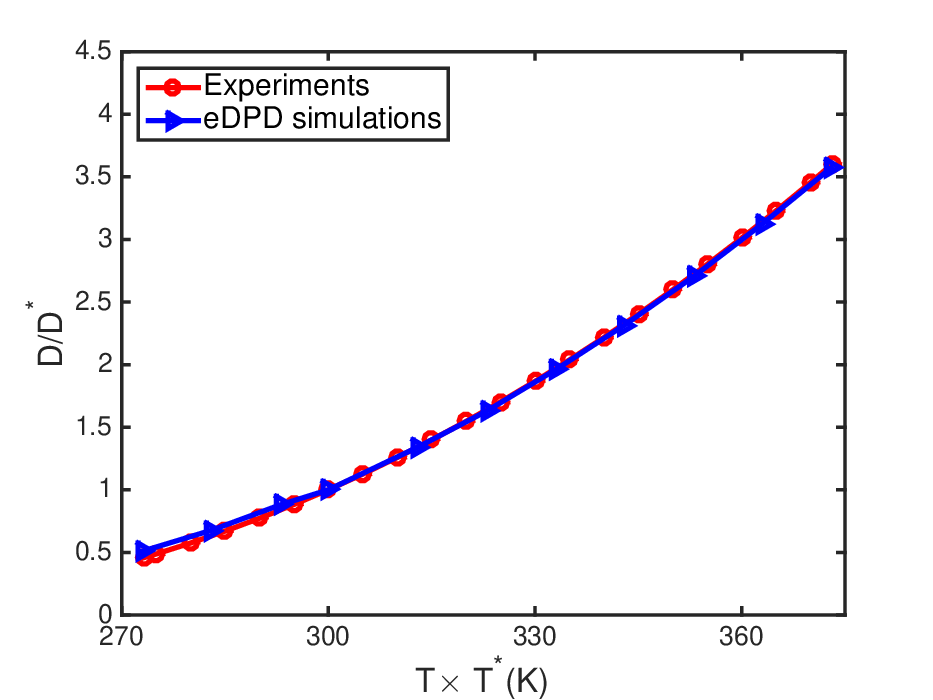
The comparisons of eDPD simulation with the experiment are presented in Figure 15. The eDPD simulation results match the experiment quite well. Especially, the relative error of the viscosity is less than at each temperature. The estimate of the diffusivity is also very accurate for , and the error grows slightly to around as approaches . These results demonstrate that with the present formulation we have improved the results in [16] by introducing an advanced model for and implementing the systematic approach to identify the parameters in the system.

5 Summary and Discussion
In this work, we employ the gPC and compressive sensing method to build accurate surrogate model efficiently for mesoscopic polymer melt systems and non-isothermal liquid water. We target various dynamic or thermal properties and show that the numerical error of the gPC expansions computed by the present method is comparable with (smaller than in some cases) the sparse grid method. Moreover, different from the sparse grid method, the present method enables us to incorporate new simulation data with no restriction on the number of new samples, which is an advantage especially for mesoscopic modeling and simulation, since in practice, the simulations are very costly and may not be available at the specific sampling points in random parameter space. On the other hand, compared with the Monte Carlo method, the present method shows much faster convergence rate (e.g., see [41, 43]) validating its high efficiency in exploiting information from limited data. These results demonstrate that the present method is well suited for studying uncertainty quantification for mesoscopic models, in particular for those with relatively high dimensional random parameter space, where only a limited number of simulations can be afforded.
Accurately recovering the gPC coefficients of the target properties over the random parameter space enables us to calibrate the model parameters with respect to the observed target property values (e.g., shear-rate viscosity, temperature-dependent viscosity and diffusivity, etc.) While a simple dumbbell FENE model is considered in the current study for demonstration purposes, the present method can be readily extended to more complex polymer melts and other soft matter models. For example, as shown in Ref. [79], we may further incorporate the more general pressure tensor by further introducing model variables such as tangential friction. For models with high dimensional random parameter space, the present work also provides a framework for model optimization/reduction through identification of all possible parameter degeneracies. We note that the dual effects from multiple parameters on target properties of the mesoscopic models may not be easily identified on the basis of pure theoretical modeling concepts. Systematic analysis on the intrinsic relationship between those parameters relies on the full and accurate access to the response surface of the targeted properties obtained from the present study.
Finally, we emphasize that several factors not considered in the present work may further affect the performance of the proposed method. First, we note that the present method relies on a prior assumption that the solution (gPC coefficients) is “sparse” in the gPC basis; otherwise, we may not be able to obtain accurate results by means of compressive sensing. However, this condition, in practice, is usually not that strong for most mesoscopic model systems. Given a system governed by a regular Hamiltonian formulation, the physical properties can usually be well approximated by low orders of polynomial function over parameter space. Second, we emphasize that the inferred parameter set for the mesoscopic model in the present work is associated with the specific target properties we aim to recover. In the polymer melt system in Sec. 4.2.2, we show that the parameter degeneracy identified from the target properties also applies to other dynamic properties. However, the general applicability of the inferred parameter set and transferability to other properties remains an open question. Essentially, the present framework enables to parameterize the free energy space of mesoscopic model, on the other hand, extension to other properties further depends on the compatibility of the free energy space with those properties. For example, to capture polydispersity and entanglement effects of long polymer chains, we need to start with some mesoscopic model where those structural properties can be (partially) characterized such that the present method can further facilitate finding the optimized model parameters. Third, we consider systems with small thermal noise in this paper. For systems with large thermal noise, we may need to adopt an appropriate method to separate model parameter induced uncertainty from the intrinsic thermal fluctuation, e.g., see Ref. [74] Finally, we note that the present work cannot be directly applied to study systems with parameter confidence range across the phase transition regime. Special treatment is needed to take care of the abrupt discontinuity near the phase transition regime. Remarkably, the present method can still be applied if we are only interested in those properties which do not undergo drastic changes across the phase transition, e.g., morphological state under Rouse reptation transition for polymer melt system [80]. All these issues need further study and will be addressed in future work.
6 Appendix
We provide a toy model further help readers to understand the procedure in Algorithms 1 and 2. Assume that we have a polymer model relying on two i.i.d. uniform random variables and with . Here takes the following form:
| (6.1) |
where is a Gaussian random variable representing the intrinsic noise. We now go through all the steps of Algorithms 1 and 2 to demonstrate how they work. Since we will use Legendre polynomial expansion to approximate , we first construct the two-dimensional normalized Legendre polynomial defined on based on the one-dimensional normalized Legendre polynomials defined on using tensor product rule. The one-dimensional normalized Legendre polynomials up to second order are: , and the two-dimensional Legendre polynomials are:
| (6.2) |
Hence, the simple polymer model can be represented as:
| (6.3) |
The coefficients vector is . We will show step by step how Algorithms 1 and 2 approximate based on the output of Monte Carlo simulations.
Steps 1 and 2: Run Monte Carlo simulation to obtain the output of the polymer model. We generate five input samples of and five samples of , then we can compute the five samples of . We note that for realistic problems, Monte Carlo simulation consists of only two parts: 1) generating input samples of ; 2) evaluating with samples of . Table 7 lists input samples and corresponding output samples .
| (0.0258,-0.0790) | (-0.2992,-0.8099) | (-0.1327,0.4185) | (-0.7681,-0.8438) | (-0.2615,-0.9327) | |
| 0.6905 | 0.4235 | 0.5822 | 0.2942 | 0.4780 |
Step 3: We construct the “measurement matrix" by evaluating two-dimensional Legendre polynomial at the samples of . More precisely, , where and . Hence, we obtain the following linear system:
| (6.4) |
Step 4: In the demonstration we choose a threshold . In practice, it is estimated by cross-validation and details can be found in [41].
Step 5: Solve the minimization by using Algorithm 1. The step by step details are as follows:
- 1.
. Then in Algorithms 1 are: . Hence, we select , and . Here which is larger than the threshold , so we need to continue expanding .
- 2.
. Then in Algorithms 1 are: . Hence, we select , and . Then, we compute the minimizer of subject to . The results is and the residual . Since is still larger than the threshold , we continue expanding .
- 3.
After five similar steps, we obtain and , hence we can stop.
Finally, we use to approximate the coefficients in the polymer model .
7 Acknowledgment
This research is sponsored by the Army Research Laboratory and was accomplished under Cooperative Agreement Number W911NF-12-2-0023 to University of Utah. We also acknowledge partial support from the new Collaboratory on Mathematics for Mesoscopic Modeling of Materials (CM4) supported by DOE. We would like to thank Hui Wang, Zhongqiang Zhang, Mingge Deng, Xiaoxing Cheng and two anonymous reviewers for helpful discussions and constructive suggestions.
References
- [1] W. L. Jorgensen, D. S. Maxwell, J. Tirado-Rives, Development and testing of the opls all-atom force field on conformational energetics and properties of organic liquids, J. Am. Chem. Soc. 118 (45) (1996) 11225–11236.
- [2] T. Spyriouni, I. G. Economou, D. N. Theodorou, Molecular simulation of -olefins using a new united-atom potential model:. vapor-liquid equilibria of pure compounds and mixtures, J. Am. Chem. Soc. 121 (14) (1999) 3407–3413.
- [3] P. Español, M. Serrano, I. Zuniga, Coarse-graining of a fluid and its relation with dissipative particle dynamics and smoothed particle dynamics, Int. J. Mod. Phys. C 8 (1997) 899–908.
- [4] S. H. L. Klapp, D. J. Diestler, M. Schoen, Why are effective potentials “soft"?, J. Phys-Condens. Mat. 16 (41) (2004) 7331–7352.
- [5] A. A. Louis, P. G. Bolhuis, J. P. Hansen, E. J. Meijer, Can polymer coils be modeled as “soft colloids"?, Phys. Rev. Lett. 85 (12) (2000) 2522–2525.
- [6] T. Kinjo, S. Hyodo, Linkage between atomistic and mesoscale coarse-grained simulation, Mol. Simulat. 33 (4-5) (2007) 417–420.
- [7] R. L. C. Akkermans, W. J. Briels, Coarse-grained interactions in polymer melts: A variational approach, J. Chem. Phys. 115 (13) (2001) 6210–6219.
- [8] V. A. Harmandaris, N. P. Adhikari, N. F. A. van der Vegt, K. Kremer, Hierarchical modeling of polystyrene: From atomistic to coarse-grained simulations, Macromolecules 39 (19) (2006) 6708–6719.
- [9] H. Fukunaga, J. Takimoto, M. Doi, A coarse-graining procedure for flexible polymer chains with bonded and nonbonded interactions, J. Chem. Phys. 116 (18) (2002) 8183–8190.
- [10] R. L. C. Akkermans, W. J. Briels, Coarse-grained dynamics of one chain in a polymer melt, J. Chem. Phys. 113 (15) (2000) 6409–6422.
- [11] H. Lei, B. Caswell, G. E. Karniadakis, Direct construction of mesoscopic models from microscopic simulations, Phys. Rev. E 81 (2010) 026704.
- [12] T. Kinjo, S. A. Hyodo, Equation of motion for coarse-grained simulation based on microscopic description, Phys. Rev. E 75 (5) (2007) 051109.
- [13] P. J. Hoogerbrugge, J. M. V. A. Koelman, Simulating microscopic hydrodynamic phenomena with dissipative particle dynamics, Europhys. Lett. 19 (3) (1992) 155–160.
- [14] P. Español, P. Warren, Statistical mechanics of dissipative particle dynamics, Europhys. Lett. 30 (4) (1995) 191–196.
- [15] R. Qiao, P. He, Simulation of heat conduction in nanocomposite using energy-conserving dissipative particle dynamics, Mol. Simul. 33 (8) (2007) 677–683.
- [16] Z. Li, Y.-H. Tang, H. Lei, B. Caswell, G. E. Karniadakis, Energy-conserving dissipative particle dynamics with temperature-dependent properties, J. Comput. Phys. 265 (2014) 113–127.
- [17] A. Eriksson, M. N. Jacobi, J. Nystrom, K. Tunstrom, Using force covariance to derive effective stochastic interactions in dissipative particle dynamics, Phys. Rev. E 77 (1) (2008) 016707.
- [18] C. Hijón, P. Español, E. Vanden-Eijnden, R. Delgado-Buscalioni, Mori-Zwanzig formalism as a practical computational tool, Farad. Discuss. 144 (2010) 301–322.
- [19] S. Izvekov, B. M. Rice, Multi-scale coarse-graining of non-conservative interactions in molecular liquids, J. Chem. Phys. 140 (10) (2014) 104104.
- [20] Z. Li, X. Bian, B. Caswell, G. E. Karniadakis, Construction of dissipative particle dynamics models for complex fluids via the mori-zwanzig formulation, Soft Matter 10 (2014) 8659–8672.
- [21] H. Mori, Transport, collective motion, and Brownian motion, Prog. Theor. Phys 33 (1965) 423.
- [22] R. Zwanzig, Ensemble method in the theory of irreversibility, J. Chem. Phys. 33 (1960) 1338.
- [23] A. Gelman, J. B. Carlin, H. S. Stern, D. B. Dunson, A. Vehtari, D. B. Rubin, Bayesian data analysis, CRC press, 2013.
- [24] J. S. Liu, Monte Carlo strategies in scientific computing, springer, 2008.
- [25] R. G. Ghanem, P. D. Spanos, Stochastic finite elements: a spectral approach, Springer-Verlag, New York, 1991.
- [26] D. Xiu, G. E. Karniadakis, The Wiener-Askey polynomial chaos for stochastic differential equations, SIAM J. Sci. Comput. 24 (2) (2002) 619–644.
- [27] Y. M. Marzouk, H. N. Najm, L. A. Rahn, Stochastic spectral methods for efficient Bayesian solution of inverse problems, J. Comput. Phys. 224 (2) (2007) 560–586.
- [28] Y. M. Marzouk, H. N. Najm, Dimensionality reduction and polynomial chaos acceleration of bayesian inference in inverse problems, J. Comput. Phys. 228 (6) (2009) 1862–1902.
- [29] F. Rizzi, H. N. Najm, B. J. Debusschere, K. Sargsyan, M. Salloum, H. Adalsteinsson, O. M. Knio, Uncertainty quantification in MD simulation. Part I: Forward propagation, Multiscale Model Simul 10 (4) (2012) 1428–1459.
- [30] F. Rizzi, H. N. Najm, B. J. Debusschere, K. Sargsyan, M. Salloum, H. Adalsteinsson, O. M. Knio, Uncertainty quantification in MD simulation. Part II: Bayesian inference of force-field parameters, Multiscale Model Simul 10 (4) (2012) 1460–1492.
- [31] D. Xiu, J. S. Hesthaven, High-order collocation methods for differential equations with random inputs, SIAM J. Sci. Comput. 27 (3) (2005) 1118–1139.
- [32] B. Ganapathysubramanian, N. Zabaras, Sparse grid collocation schemes for stochastic natural convection problems, J. Comput. Phys. 225 (1) (2007) 652–685.
- [33] J. Foo, X. Wan, G. E. Karniadakis, The multi-element probabilistic collocation method (ME-PCM): error analysis and applications, J. Comput. Phys. 227 (22) (2008) 9572–9595.
- [34] F. Nobile, R. Tempone, C. G. Webster, An anisotropic sparse grid stochastic collocation method for partial differential equations with random input data, SIAM J. Numer. Anal. 46 (5) (2008) 2411–2442.
- [35] X. Ma, N. Zabaras, An adaptive hierarchical sparse grid collocation algorithm for the solution of stochastic differential equations, J. Comput. Phys. 228 (8) (2009) 3084–3113.
- [36] X. Ma, N. Zabaras, An adaptive high-dimensional stochastic model representation technique for the solution of stochastic partial differential equations, J. Comput. Phys. 229 (10) (2010) 3884–3915.
- [37] J. Foo, G. E. Karniadakis, Multi-element probabilistic collocation method in high dimensions, J. Comput. Phys. 229 (5) (2010) 1536–1557.
- [38] Z. Zhang, M. Choi, G. E. Karniadakis, Error estimates for the ANOVA method with polynomial chaos interpolation: Tensor product functions, SIAM J. Sci. Comput. 34 (2) (2012) A1165–A1186.
- [39] X. Yang, M. Choi, G. Lin, G. E. Karniadakis, Adaptive ANOVA decomposition of stochastic incompressible and compressible flows, J. Comput. Phys. 231 (4) (2012) 1587 – 1614.
- [40] X. Li, Finding deterministic solution from underdetermined equation: large-scale performance variability modeling of analog/rf circuits, Computer-Aided Design of Integrated Circuits and Systems, IEEE Transactions on 29 (11) (2010) 1661–1668.
- [41] A. Doostan, H. Owhadi, A non-adapted sparse approximation of PDEs with stochastic inputs, J. Comput. Phys. 230 (8) (2011) 3015–3034.
- [42] L. Yan, L. Guo, D. Xiu, Stochastic collocation algorithms using -minimization, Int. J. Uncertainty Quantification 2 (3) (2012) 279–293.
- [43] X. Yang, G. E. Karniadakis, Reweighted minimization method for stochastic elliptic differential equations, J. Comput. Phys. 248 (1) (2013) 87 – 108.
- [44] H. Lei, X. Yang, B. Zheng, G. Lin, N. A. Baker, Constructing surrogate models of complex systems with enhanced sparsity: Quantifying the influence of conformational uncertainty in biomolecular solvation, SIAM Multiscale Model. Simul. 13 (4) (2015) 1327–1353.
- [45] X. Yang, H. Lei, N. A. Baker, G. Lin, Enhancing sparsity of hermite polynomial expansions by iterative rotations, J. Comput. Phys. 307 (2016) 94–109.
- [46] E. J. Candès, T. Tao, Decoding by linear programming, IEEE Trans. Inform. Theory 51 (12) (2005) 4203–4215.
- [47] E. J. Candes, J. K. Romberg, T. Tao, Stable signal recovery from incomplete and inaccurate measurements, Comm. Pur. Appl. Math. 59 (8) (2006) 1207–1223.
- [48] D. L. Donoho, M. Elad, V. N. Temlyakov, Stable recovery of sparse overcomplete representations in the presence of noise, IEEE Trans. Inform. Theory 52 (1) (2006) 6–18.
- [49] A. M. Bruckstein, D. L. Donoho, M. Elad, From sparse solutions of systems of equations to sparse modeling of signals and images, SIAM Rev. 51 (1) (2009) 34–81.
- [50] R. D. Groot, P. B. Warren, Dissipative particle dynamics: Bridging the gap between atomistic and mesoscopic simulation, J. Chem. Phys. 107 (11) (1997) 4423–4435.
- [51] N. A. Spenley, Scaling laws for polymers in dissipative particle dynamics, Europhys. Lett. 49 (4) (2000) 534.
- [52] X. Fan, N. Phan-Thien, S. Chen, X. Wu, T. Y. Ng, Simulating flow of DNA suspension using dissipative particle dynamics, Phys. Fluids 18 (6) (2006) 063102.
- [53] V. Symeonidis, G. E. Karniadakis, B. Caswell, Dissipative particle dynamics simulations of polymer chains: Scaling laws and shearing response compared to DNA experiments, Phys. Rev. Lett. 95 (7) (2005) 076001.
- [54] I. V. Pivkin, P. D. Richardson, G. E. Karniadakis, Effect of red blood cells on platelet aggregation, Engin. Med. Biol. Magazine, IEEE 28 (2) (2009) 32 –37.
- [55] A. C. Brown, S. E. Stabenfeldt, B. Ahn, R. T. Hannan, K. S. Dhada, E. S. Herman, V. Stefanelli, N. Guzzetta, A. Alexeev, W. A. Lam, L. A. Lyon, T. H. Barker, Ultrasoft microgels displaying emergent platelet-like behaviours, Nat. Mater. 13 (12) (2014) 1108–1114.
- [56] E. S. Boek, P. V. Coveney, H. N. W. Lekkerkerker, P. van der Schoot, Simulating the rheology of dense colloidal suspensions using dissipative particle dynamics, Phys. Rev. E 55 (3) (1997) 3124–3133.
- [57] Z. Li, G.-H. Hu, Z.-L. Wang, Y.-B. Ma, Z.-W. Zhou, Three dimensional flow structures in a moving droplet on substrate: A dissipative particle dynamics study, Phys. Fluids 25 (7) (2013) 072103.
- [58] I. V. Pivkin, G. E. Karniadakis, Accurate coarse-grained modeling of red blood cells, Phys. Rev. Lett. 101 (11) (2008) 118105.
- [59] D. A. Fedosov, B. Caswell, G. E. Karniadakis, A multiscale red blood cell model with accurate mechanics, rheology, and dynamics, Biophysical Journal 98 (10) (2010) 2215–2225.
- [60] D. A. Fedosov, B. Caswell, S. Suresh, G. E. Karniadakis, Quantifying the biophysical characteristics of plasmodium-falciparum-parasitized red blood cells in microcirculation, Proceedings of the National Academy of Sciences 108 (2010) 35–39.
- [61] H. Lei, G. E. Karnidakis, Quantifying the rheological and hemodynamic characteristics of sickle cell anemia, Biophys. J. 102 (2012) 185–194.
- [62] H. Lei, G. E. Karniadakis, Probing vasoocclusion phenomena in sickle cell anemia via mesoscopic simulations, Proc. Natl. Acad. Sci. 110 (28) (2013) 11326–11330.
- [63] P. Español, Dissipative particle dynamics with energy conservation, Europhys. Lett. 40 (6) (1997) 631–636.
- [64] M. Ripoll, P. Español, M. H. Ernst, Dissipative particle dynamics with energy conservation: Heat conduction, Int. J. Mod. Phys. C 9 (8) (1998) 1329–1338.
- [65] P. He, R. Qiao, Self-consistent fluctuating hydrodynamics simulations of thermal transport in nanoparticle suspensions, J. Appl. Phys. 103 (9) (2008) 094305.
- [66] E. Abu-Nada, Natural convection heat transfer simulation using energy conservative dissipative particle dynamics, Phys. Rev. E 81 (5) (2010) 056704.
- [67] A. W. Lees, S. F. Edwards, The computer study of transport processes under extreme conditions, J. Phys. C 5 (1972) 1921–1928.
- [68] R. G. Larson, The Structure and Rheology of Complex Fluids, Oxford University Press, 1998.
- [69] D. A. Fedosov, B. Caswell, G. E. Karniadakis, Steady shear rheometry of dissipative particle dynamics models of polymer fluids in reverse Poiseuille flow, J. Chem. Phys. 132 (2010) 144103.
- [70] J. A. Backer, C. P. Lowe, H. C. J. Hoefsloot, P. D. Iedema, Poiseuille flow to measure the viscosity of particle model fluids, J. Chem. Phys. 122 (15) (2005) 154503–154509.
- [71] M. Holz, S. R. Heil, A. Sacco, Temperature-dependent self-diffusion coefficients of water and six selected molecular liquids for calibration in accurate H-1 NMR PFG measurements, Phys. Chem. Chem. Phys. 2 (20) (2000) 4740–4742.
- [72] T. L. Bergman, A. S. Lavine, F. P. Incropera, D. P. DeWitt, Introduction to Heat Transfer, 6th Edition, John Wiley and Sons, 2011.
- [73] D. Donoho, I. Drori, V. Stodden, Y.Tsaig, Sparselab: Seeking sparse solutions to linear systems of equations, http://www-stat.stanford.edu/~sparselab/.
- [74] O. L. Maître, O. Knio, PC analysis of stochastic differential equations driven by Wiener noise, Reliability Engineering & System Safety 135 (2015) 107 – 124.
- [75] H. Haario, E. Saksman, J. Tamminen, An adaptive metropolis algorithm, Bernoulli (2001) 223–242.
- [76] H. Haario, M. Laine, A. Mira, E. Saksman, Dram: efficient adaptive mcmc, Stat. Comput. 16 (4) (2006) 339–354.
- [77] J. Ching, Y. Chen, Transitional markov chain monte carlo method for bayesian model updating, model class selection, and model averaging, Journal of Engineering Mechanics 133 (7) (2007) 816–832.
- [78] P. Angelikopoulos, C. Papadimitriou, P. Koumoutsakos, Bayesian uncertainty quantification and propagation in molecular dynamics simulations: A high performance computing framework, J. Chem. Phys. 137 (14) (2012) 144103.
- [79] J. Sablic, M. Praprotnik, R. Delgado-Buscalioni, Open boundary molecular dynamics of sheared star-polymer melts, Soft Matter 12 (2016) 2416–2439.
- [80] We thank the anonymous referees for bringing up these good points.