跳到论文正文
W Papers独立论文阅读器 arXiv:1606.06754 论文正文 计算阅读时间 · 0%
引用这篇论文根据当前论文元数据生成,正式投稿前建议核对。


License: arXiv.org perpetual non-exclusive license
arXiv:1606.06754v2 [hep-ph] 14 Nov 2016

DESY 16-106, TTP16-023 MS¯\overline{\rm MS}-on-shell quark mass relation up to four loops in QCD and a general SU(N)(N) gauge group

Peter Marquard    Alexander V. Smirnov    Vladimir A. Smirnov    Matthias Steinhauser    David Wellmann(a) Deutsches Elektronen-Synchrotron, DESY 15738 Zeuthen, Germany(b) Research Computing Center, Moscow State University119991, Moscow, Russia(c) Skobeltsyn Institute of Nuclear Physics of Moscow State University119991, Moscow, Russia(d) Institut für Theoretische Teilchenphysik, Karlsruhe Institute of Technology (KIT)76128 Karlsruhe, Germany
Abstract

We compute the relation between heavy quark masses defined in the modified minimal subtraction and the on-shell schemes. Detailed results are presented for all coefficients of the SU(Nc)(N_{c}) colour factors. The reduction of the four-loop on-shell integrals is performed for a general QCD gauge parameter. Altogether there are about 380 master integrals. Some of them are computed analytically, others with high numerical precision using Mellin-Barnes representations, and the rest numerically with the help of FIESTA. We discuss in detail the precise numerical evaluation of the four-loop master integrals. Updated relations between various short-distance masses and the MS¯\overline{\rm MS} quark mass to next-to-next-to-next-to-leading order accuracy are provided for the charm, bottom and top quarks. We discuss the dependence on the renormalization and factorization scale.

PACS numbers: 12.38.Bx, 12.38.Cy, 14.65.Fy, 14.65.Ha

1 Introduction

Quark masses are fundamental parameters of Quantum Chromodynamics (QCD) and thus it is mandatory to determine their numerical values as precisely as possible. Furthermore, it is important to have precise relations at hand which relate the masses in different renormalization schemes.

The renormalization scheme for the quark masses has to be fixed once quantum corrections are considered. In QCD there are two distinct renormalization schemes for the quark masses: the on-shell (OS) scheme, which is motivated by the physical interpretation of the mass parameter, and the modified minimal subtraction (MS¯\overline{\rm MS}) scheme which is very convenient for many practical calculations, in particular in high-energy processes.

In the case of the lighter quarks (up, down and strange) the meson masses are in general much larger than the masses of the quarks. Thus, the concept of the on-shell scheme is not applicable to light quark flavours; their numerical values are usually given in the MS¯\overline{\rm MS} scheme. On the other hand, the masses of the mesons involving charm and bottom quarks are essentially dominated by the quark masses. For this reason, the quantum corrections considered in this paper are mainly relevant for the three heavy quarks, charm, bottom and top.

The top quark plays a special role in this context. Due to its large width it decays before hadronization and thus can be considered as an almost free quark. As a consequence it can be expected that the on-shell value for the top quark can be determined with a relatively small uncertainty. This aspect has been studied in detail in recent papers [1, 2]. It has been shown that the on-shell top quark can be computed from the MS¯\overline{\rm MS} mass with an irreducible uncertainty of about 70 MeV [2].

There are various methods which can be used to obtain numerical values for the quark masses. Some of them determine directly the MS¯\overline{\rm MS} quark mass (see, e.g., Ref. [3]) and thus do not suffer from the inherent renormalon ambiguity. However, the highest sensitivity to the quark masses is in general obtained from physical quantities evaluated at energies close to the quark mass. In such situations it is convenient to introduce so-called threshold masses to parametrize the physical quantities. Among the most prominent ones are the potential subtracted (PS) [4], 1S [5, 6, 7], renormalon subtracted (RS) [8] and the kinetic mass [9].11 1 Note that the relation of the kinetic mass to the on-shell mass is currently only known to NNLO. For this reason it will not be considered in the following. They allow for a precise determination of the heavy MS¯\overline{\rm MS} mass without explicit reference to the pole quark mass. However, at intermediate stages the pole mass and, in particular, the relation between the pole and the MS¯\overline{\rm MS} mass is still needed.

In the following we describe three typical examples where the four-loop terms in the mass relations turn out to be important.

  • •

    At the TEVATRON and the LHC the top quark mass is measured with an uncertainty below 1 GeV. For example, the combination of results from ATLAS, CDF, CMS and D0 from March 2014 [10] leads to

    Mt\displaystyle M_{t} =\displaystyle= 173.34±0.27​(stat)±0.71​(syst)​GeV,\displaystyle 173.34\pm 0.27({\rm stat})\pm 0.71({\rm syst})~\mbox{GeV}\,, (1)

    with a total uncertainty of 760 MeV. The value in Eq. (1) is often called “Monte-Carlo mass” and there are several attempts which suggest methods to relate it to the on-shell mass (see, e.g., Refs. [11, 12, 13]). In case Eq. (1) is interpreted as the on-shell quark mass it has to be converted to the MS¯\overline{\rm MS} top quark mass. Note that the three-loop term in the conversion formulae contributes approximately 500500 MeV which is of the same order as the experimental uncertainties in Eq. (1).

  • •

    From measurements of the top quark pair production cross section close to threshold at a future linear collider it will be possible to determine the top quark threshold mass with an accuracy below 100 MeV (see, e.g., Refs. [14, 15]). In the conversion to the MS¯\overline{\rm MS} definition there is a contribution of about 150-200 MeV from the three-loop term in the mass relations which contributes significantly to the final uncertainty of the MS¯\overline{\rm MS} mass (see Section 4.2 for precise numbers). With the help of the four-loop MS¯\overline{\rm MS}-on-shell relation this uncertainty can be drastically reduced.

    For the sake of completeness let us mention that there is an approach to determine directly the MS¯\overline{\rm MS} top quark mass from the threshold cross section (see, e.g., Ref. [16]). In future it will be interesting to compare the top quark mass values obtained with different methods.

  • •

    The bottom quark mass can be extracted from Υ\Upsilon sum rules (see Refs. [17, 18] for recent N3LO analyses) and from M⁡(Υ⁡(1​S))M(\Upsilon(1S)) [19, 20, 21, 22]. Usually, in a first step a threshold mass is obtained. To be able to compare with the MS¯\overline{\rm MS} quark mass (as, e.g., extracted from low-moment sum rules [3]) one has to apply the corresponding conversion formula. At three loops the contribution is of the order of 30 MeV, which is of the same order of magnitude (in some cases even larger) than the combination of all other uncertainties involved.

These examples show that the three-loop contribution is sizeable and a reliable estimate of the uncertainty is only obtained once the four-loop corrections are available. Furthermore, note that for the PS, 1S and RS masses one knows the relation to the pole mass to N3LO. However, due to strong cancellations (see below) the N3LO term cannot be used unless four-loop corrections to the MS¯\overline{\rm MS} and on-shell quark mass are available.

The remainder of the paper is organized as follows: In the next Section we introduce the conversion factor between the on-shell and the MS¯\overline{\rm MS} mass and discuss the colour decomposition of the four-loop term. Furthermore, we provide several technical details and discuss, in particular, the numerical accuracy of the master integrals. Section 3 is devoted to the results of the MS¯\overline{\rm MS}-on-shell relation which we discuss for the physical limit, i.e. Nc=3N_{c}=3 and fixed number of massless quarks, nln_{l}, but also for generic NcN_{c} and even for general SU(Nc)(N_{c}) colour factors. Several applications of the MS¯\overline{\rm MS}-on-shell relation are discussed in Section 4 and our conclusions are contained in Section 5.

2 Technicalities

2.1 Mass relations

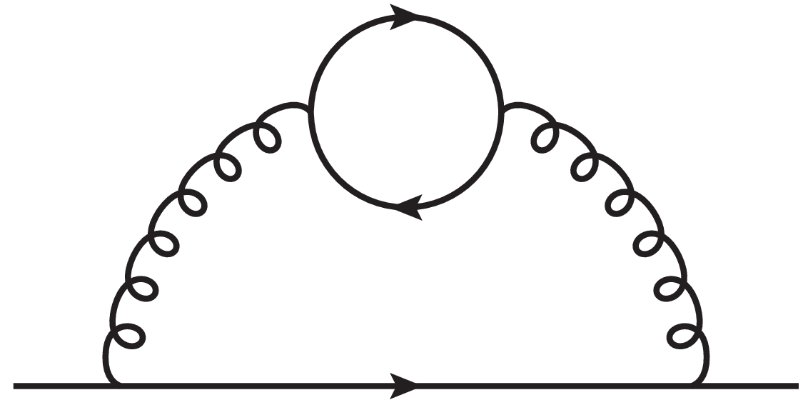
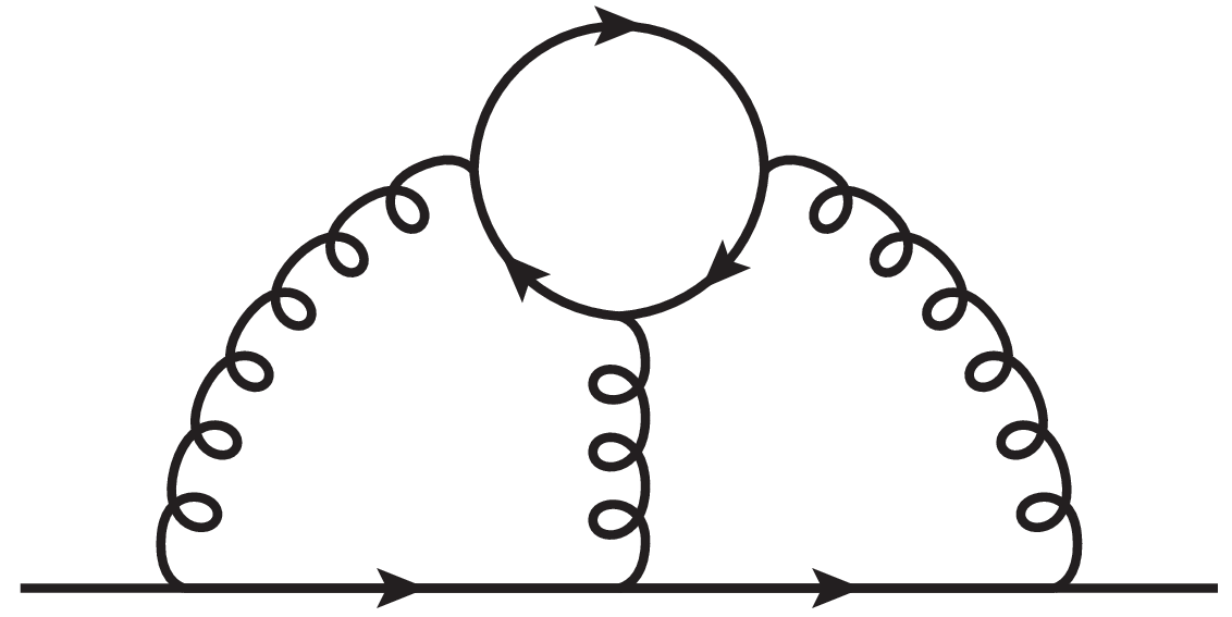
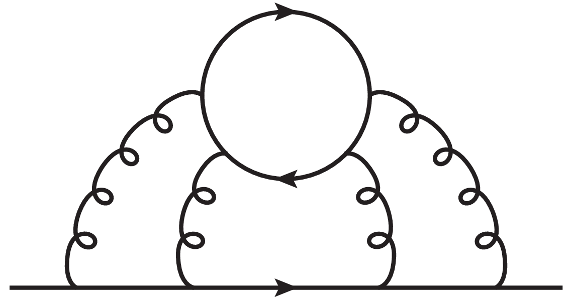
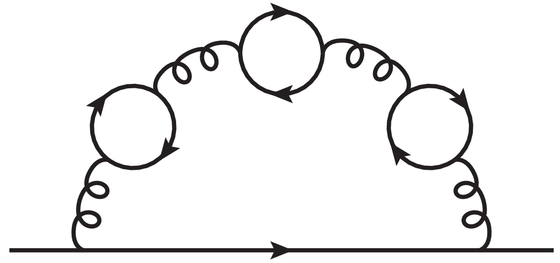
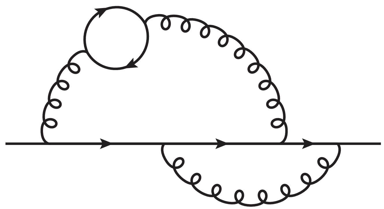
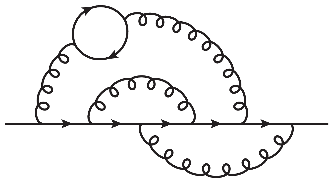
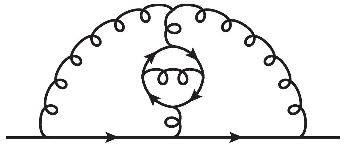
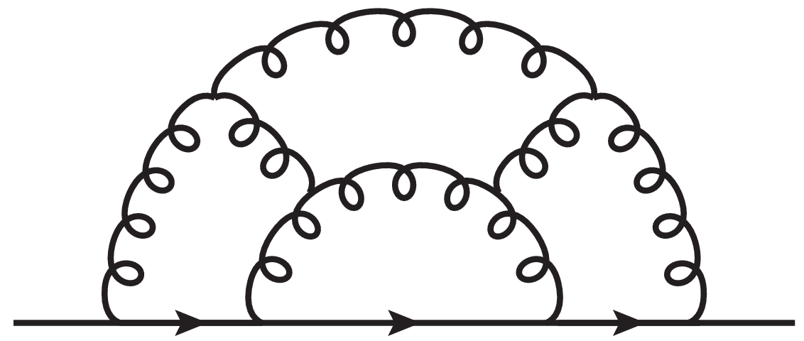
Refer to caption Refer to caption Refer to caption Refer to caption
Figure 1: Sample Feynman diagrams contributing to ΣS\Sigma_{S} and ΣV\Sigma_{V} at one-, two-, three- and four-loop order. The solid lines represent quarks and the curly lines gluons.

The relation between the bare (m0m_{0}) and renormalized mass in the MS¯\overline{\rm MS} scheme (mm) is given by

m0=ZmMS¯​m,\displaystyle m_{0}=Z_{m}^{\overline{\rm MS}}m\,, (2)

where ZmMS¯Z_{m}^{\overline{\rm MS}} only contains poles in ϵ\epsilon. It is obtained by requiring that the renormalized propagator is finite. Note that in QCD the fermion propagator contains two Lorenz structures (scalar and vector). Thus next to ZmMS¯Z_{m}^{\overline{\rm MS}} also the MS¯\overline{\rm MS} wave function renormalization constant is determined. ZmMS¯Z_{m}^{\overline{\rm MS}} has been computed to five-loop order in Ref. [23]; for our calculation only four-loop corrections [24, 25, 26] are needed. We use ZmMS¯Z_{m}^{\overline{\rm MS}} expressed for generic SU(Nc)(N_{c}) colour factors which can be extracted from the anomalous dimension given in [25]. For convenience we present the result for ZmMS¯{Z_{m}^{\overline{\rm MS}}} in Appendix F. Note that the MS¯\overline{\rm MS}-renormalized mass mm depends on the renormalization scale μ\mu which is suppressed in Eq. (2). ZmMS¯Z_{m}^{\overline{\rm MS}} depends on μ\mu via the strong coupling constant αs​(μ)\alpha_{s}(\mu).

In the on-shell renormalization scheme one requires that the quark two-point function vanishes at the position of the on-shell mass MM which fixes the renormalization constant ZmOSZ_{m}^{\rm OS} introduced via

m0=ZmOS​M.\displaystyle m_{0}=Z_{m}^{\rm OS}M\,. (3)

Note that m0m_{0} and MM are μ\mu-independent and ZmOSZ_{m}^{\rm OS} contains αs​(μ)\alpha_{s}(\mu) and log⁡(μ/M)\log(\mu/M) terms. The on-shell wave function renormalization constant is determined from the requirement that the quark propagator has a residue −i-i at q2=M2q^{2}=M^{2}. This leads to a formula for Z2OSZ_{2}^{\rm OS} which is independent of ZmOSZ_{m}^{\rm OS}. This is different in the MS¯\overline{\rm MS} scheme where ZmMS¯Z_{m}^{\overline{\rm MS}} and Z2MS¯Z_{2}^{\overline{\rm MS}} have to be determined simultaneously.

A formula for ZmOSZ_{m}^{\rm OS} is conveniently derived by considering the renormalized quark propagator

SF​(q)\displaystyle S_{F}(q) =\displaystyle= −i​Z2OSq/−mq,0+Σ(q,M),\displaystyle\frac{-iZ_{2}^{\rm OS}}{q\!\!\!/\,\,-m_{q,0}+\Sigma(q,M)}\,, (4)

Σ⁡(q,M)\Sigma(q,M) is the (amputated) quark self energy which can be split into a scalar and vector contribution

Σ⁡(q,M)\displaystyle\Sigma(q,M) =\displaystyle= M​ΣS​(q2,M)+q/ΣV​(q2,M),\displaystyle M\,\Sigma_{S}(q^{2},M)+q\!\!\!/\,\,\,\Sigma_{V}(q^{2},M)\,, (5)

where ΣS\Sigma_{S} and ΣV\Sigma_{V} only depend of q2q^{2}, the (renormalized) quark mass and μ\mu (which is again suppressed). They are obtained from the self energy Σ\Sigma with the help of the projectors

ΣS​((M2,M)CLOSE\displaystyle\Sigma_{S}((M^{2},M) =\displaystyle= 14​M​Tr​(Σ⁡(q,M))|q2=M2,\displaystyle\frac{1}{4M}\,\mbox{Tr}\,\left(\Sigma(q,M)\right)\Bigg|_{q^{2}=M^{2}}\,, (6)
ΣV​((M2,M)CLOSE\displaystyle\Sigma_{V}((M^{2},M) =\displaystyle= 14​q2​Tr​(q/Σ⁡(q,M))|q2=M2.\displaystyle\frac{1}{4q^{2}}\,\mbox{Tr}\,\left(q\!\!\!/\,\,\,\Sigma(q,M)\right)\Bigg|_{q^{2}=M^{2}}\,. (7)

Sample Feynman diagrams contributing to Σ⁡(q,M)\Sigma(q,M) are shown in Fig. 1.

Requiring that the inverse quark propagator, [SF​(q)]−1\left[S_{F}(q)\right]^{-1} vanishes at the position of the on-shell mass, i.e.

SF​(q)\displaystyle S_{F}(q) ⟶q2→M2\displaystyle\stackrel{{\scriptstyle q^{2}\to M^{2}}}{{\longrightarrow}} −iq/−M,\displaystyle\frac{-i}{q\!\!\!/\,\,-M}\,, (8)

leads to

ZmOS\displaystyle Z_{m}^{\rm OS} =\displaystyle= 1+ΣS​(M2,M)+ΣV​(M2,M).\displaystyle 1+\Sigma_{S}(M^{2},M)+\Sigma_{V}(M^{2},M)\,. (9)

Thus, for the evaluation of the nn-loop contribution to ZmOSZ_{m}^{\rm OS} nn-loop on-shell integrals have to be computed.

In this paper we present results for the finite quantity

zm​(μ)\displaystyle z_{m}(\mu) =\displaystyle= m⁡(μ)M=ZmOSZmMS¯,\displaystyle\frac{m(\mu)}{M}\,\,=\,\,\frac{Z_{m}^{\rm OS}}{Z_{m}^{\overline{\rm MS}}}\,, (10)

which is obtained from Eqs. (2) and (9). Note that zm​(μ)z_{m}(\mu) depends on αs​(μ)\alpha_{s}(\mu) and log⁡(μ/M)\log(\mu/M) and has the following perturbative expansion

zm​(μ)\displaystyle z_{m}(\mu) =\displaystyle= ∑n≥0(αs​(μ)π)n​zm(n)​(μ),\displaystyle\sum_{n\geq 0}\left(\frac{\alpha_{s}(\mu)}{\pi}\right)^{n}z_{m}^{(n)}(\mu)\,, (11)

with zm(0)=1z_{m}^{(0)}=1. For later convenience we decompose zm(n)​(μ)z_{m}^{(n)}(\mu) into

zm(n)​(μ)\displaystyle z_{m}^{(n)}(\mu) =\displaystyle= zm(n)​(M)+zm(n),log,\displaystyle z_{m}^{(n)}(M)+z_{m}^{(n),\rm log}\,, (12)

where the second term on the right-hand side comprises the μ\mu-dependent terms which vanish for μ=M\mu=M. Analytic results for zm(n),logz_{m}^{(n),\rm log} are given in Appendix C.

For later use we also introduce the inverted relation to Eq. (10)

cm​(μ)\displaystyle c_{m}(\mu) =\displaystyle= Mm⁡(μ),\displaystyle\frac{M}{m(\mu)}\,, (13)

with

cm​(μ)\displaystyle c_{m}(\mu) =\displaystyle= ∑n≥0(αs​(μ)π)n​cm(n)​(μ),\displaystyle\sum_{n\geq 0}\left(\frac{\alpha_{s}(\mu)}{\pi}\right)^{n}c_{m}^{(n)}(\mu)\,, (14)

and cm(0)=1c_{m}^{(0)}=1. cm(n)​(μ)c_{m}^{(n)}(\mu) is a function of log⁡(μ/m⁡(μ))\log(\mu/m(\mu)). Furthermore, we assume the similar decomposition of Eq. (12) with cm(n),log=0c_{m}^{(n),\rm log}=0 for μ=m⁡(m)\mu=m(m).

In this paper we consider generic SU(Nc)(N_{c}) colour factors and present results for the coefficients. The four-loop term of Eq. (11) can be decomposed into 23 colour structures which are given by

zm(4)\displaystyle z_{m}^{(4)} =\displaystyle= CF4​zmF​F​F​F+CF3​CA​zmF​F​F​A+CF2​CA2​zmF​F​A​A+CF​CA3​zmF​A​A​A\displaystyle C_{F}^{4}z_{m}^{FFFF}+C_{F}^{3}C_{A}z_{m}^{FFFA}+C_{F}^{2}C_{A}^{2}z_{m}^{FFAA}+C_{F}C_{A}^{3}z_{m}^{FAAA} (15)
+dFa​b​c​d​dAa​b​c​dNc​zmdF​A+nl​dFa​b​c​d​dFa​b​c​dNc​zmdF​F​L+nh​dFa​b​c​d​dFa​b​c​dNc​zmdF​F​H\displaystyle\mbox{}+\frac{d_{F}^{abcd}d_{A}^{abcd}}{N_{c}}z_{m}^{d_{FA}}+n_{l}\frac{d_{F}^{abcd}d_{F}^{abcd}}{N_{c}}z_{m}^{d_{FF}L}+n_{h}\frac{d_{F}^{abcd}d_{F}^{abcd}}{N_{c}}z_{m}^{d_{FF}H}
+CF3​T​nl​zmF​F​F​L+CF2​CA​T​nl​zmF​F​A​L+CF​CA2​T​nl​zmF​A​A​L\displaystyle\mbox{}+C_{F}^{3}Tn_{l}z_{m}^{FFFL}+C_{F}^{2}C_{A}Tn_{l}z_{m}^{FFAL}+C_{F}C_{A}^{2}Tn_{l}z_{m}^{FAAL}
+CF2​T2​nl2​zmF​F​L​L+CF​CA​T2​nl2​zmF​A​L​L+CF​T3​nl3​zmF​L​L​L\displaystyle\mbox{}+C_{F}^{2}T^{2}n_{l}^{2}z_{m}^{FFLL}+C_{F}C_{A}T^{2}n_{l}^{2}z_{m}^{FALL}+C_{F}T^{3}n_{l}^{3}z_{m}^{FLLL}
+CF3​T​nh​zmF​F​F​H+CF2​CA​T​nh​zmF​F​A​H+CF​CA2​T​nh​zmF​A​A​H\displaystyle\mbox{}+C_{F}^{3}Tn_{h}z_{m}^{FFFH}+C_{F}^{2}C_{A}Tn_{h}z_{m}^{FFAH}+C_{F}C_{A}^{2}Tn_{h}z_{m}^{FAAH}
+CF2​T2​nh2​zmF​F​H​H+CF​CA​T2​nh2​zmF​A​H​H+CF​T3​nh3​zmF​H​H​H\displaystyle\mbox{}+C_{F}^{2}T^{2}n_{h}^{2}z_{m}^{FFHH}+C_{F}C_{A}T^{2}n_{h}^{2}z_{m}^{FAHH}+C_{F}T^{3}n_{h}^{3}z_{m}^{FHHH}
+CF2​T2​nl​nh​zmF​F​L​H+CF​CA​T2​nl​nh​zmF​A​L​H+CF​T3​nl2​nh​zmF​L​L​H\displaystyle\mbox{}+C_{F}^{2}T^{2}n_{l}n_{h}z_{m}^{FFLH}+C_{F}C_{A}T^{2}n_{l}n_{h}z_{m}^{FALH}+C_{F}T^{3}n_{l}^{2}n_{h}z_{m}^{FLLH}
+CF​T3​nl​nh2​zmF​L​H​H,\displaystyle\mbox{}+C_{F}T^{3}n_{l}n_{h}^{2}z_{m}^{FLHH}\,,

where CFC_{F} and CAC_{A} are the eigenvalues of the quadratic Casimir operators of the fundamental and adjoint representation for the SU(Nc)(N_{c}) colour group, respectively, T=1/2T=1/2 is the index of the fundamental representation, and nln_{l} and nhn_{h} count the number of massless and massive (with mass MM) quarks. In the applications discussed in Section 4 we will use nh=1n_{h}=1. It is nevertheless convenient to keep the variable nhn_{h} as a parameter. dFa​b​c​dd_{F}^{abcd} and dAa​b​c​dd_{A}^{abcd} are the symmetrized traces of four generators in the fundamental and adjoint representation, respectively. The colour structures in Eq. (15) are related to NcN_{c} via22 2 Note that our results are also valid for other groups. The corresponding expressions can easily be obtained by the proper choice of the group theory factors, see, e.g., Ref. [27]. We restrict ourselves to SU(Nc)(N_{c}) since it is closely connected to QCD. (see, e.g., Ref. [27])

CF=Nc2−12​Nc,CA=Nc,T=12,\displaystyle C_{F}=\frac{N_{c}^{2}-1}{2N_{c}}\,,\qquad C_{A}=N_{c}\,,\qquad T=\frac{1}{2}\,,
dFa​b​c​d​dFa​b​c​d=(Nc2−1)​(Nc4−6​Nc2+18)96​Nc2,\displaystyle d_{F}^{abcd}d_{F}^{abcd}=\frac{(N_{c}^{2}-1)(N_{c}^{4}-6N_{c}^{2}+18)}{96N_{c}^{2}}\,,
dFa​b​c​d​dAa​b​c​d=Nc​(Nc2−1)​(Nc2+6)48.\displaystyle d_{F}^{abcd}d_{A}^{abcd}=\frac{N_{c}(N_{c}^{2}-1)(N_{c}^{2}+6)}{48}\,. (16)

In the case of QCD we have Nc=3N_{c}=3.

One-, two- and three-loop QCD results to ZmOSZ_{m}^{\rm OS} have been computed in Refs. [28], [29] and [30, 31, 32, 33], respectively, and electroweak effects have been considered in Refs. [34, 35, 36, 37, 38, 39, 40, 41, 42, 43]. In Ref. [44] the four-loop results for zmz_{m} have been presented for Nc=3N_{c}=3 and nl=3,4n_{l}=3,4 and 55 with a numerical precision of 3% in the four-loop coefficient evaluated at μ=M\mu=M. It is the aim of the present paper to generalize the findings of [44] to general NcN_{c} and arbitrary nln_{l}. Furthermore, the precision is significantly improved. In this paper we will not study light-quark mass effects which are known at two [29] and three loops [45].

The relations between the threshold and the MS¯\overline{\rm MS} masses are too long so that we refrain from printing them in explicit form. For practical purposes it is convenient to use their implementation in RunDec [46] and CRunDec [47]. The construction of the relations can be found in the original literature [4, 5, 6, 7, 8], a summary can be found in, e.g., Ref. [44].

2.2 Reduction to master integrals

For the calculation of ΣS\Sigma_{S} and ΣV\Sigma_{V} we use a highly automated and well-established set-up based on qgraf [48], q2e and exp [49, 50] and in-house Mathematica and FORM [51, 52] programs which work hand-in-hand to minimize the manual interaction. Colour factors are computed with the help of color [27].

We use qgraf for the generation of the 3100 fermion self energy amplitudes. They are converted to FORM code using q2e and exp. A further task of the program exp is to map each diagram to one out of a set of 102 predefined integral families which are shown in graphical form in Appendix A. To obtain these families we start with the 11 prototypes shown in Fig. 2. They serve as the basis to generate the allowed families by considering all possible routings of a massive line through the diagrams. Diagrams with self-energy insertions can be obtained from the ones in Fig. 2 by removing some lines and raising the propagator powers of other lines. For convenience we show a pictorial representation for each family in Appendix A. At four loops, they are labeled by 14 indices, that correspond to powers of propagators and irreducible numerators. The maximal number of positive indices is eleven.

Refer to caption
Figure 2: Four-loop prototype families needed to generate the four-loop on-shell integral families shown in Appendix A.

We use in-house FORM programs to apply the projectors to the vector and scalar parts of the fermion propagator needed for the calculation of the on-shell quark mass, to perform traces and to decompose the scalar products in the numerator in terms of denominator factors. As an outcome our result is written as a linear combination of scalar Feynman integrals which are related by integration-by-parts identities [53]. We apply to each family the Laporta algorithm [54] as implemented in FIRE [55, 56, 57] and Crusher [58] to perform a reduction to master integrals.

We first work with each of the individual families and determine the corresponding master integrals. It turns out that the primary sets of the master integrals revealed with FIRE are not minimal, i.e. there exist additional relations among them. Then, following Ref. [56], we find additional relations using symmetries of various integrals with indices 0,10,1, and 22. For each sector33 3 A sector is a subset of indices where some indices are positive and the other indices are non-positive. one can estimate the number of the master integrals using the code Mint [59]. There are, however, additional relations which connect master integrals of partially overlapping sectors and they can be revealed by the same procedure based on symmetries. The number of the master integrals in a given family can be as large as 176.

One more criterion when looking for additional relations is the absence of a spurious dependence of denominators in reduction relations on dd. The general analysis of singularities of Feynman integrals as functions of dd shows that poles in dd can be only real rational numbers. So, if we observe a non-factorizable polynomial of second or higher degree in dd in a denominator this means that either we miss a relation between the current master integrals or some master integrals are chosen in an inappropriate way. At least in all the cases in our calculation, we managed to get rid of such spurious denominators by revealing additional relations or making better choices of the master integrals. However, with the sets of master integrals we have arrived at it is not guaranteed that we have really minimal sets of master integrals, i.e. bases of the corresponding linear spaces.

The next step was to find relations between master integrals of various families. To do this, we used the Mathematica code tsort which is part of the latest FIRE version [57] and end up with 386 four-loop massive on-shell propagator integrals, i.e. with q2=M2q^{2}=M^{2}.

We have performed the calculation allowing for a general gauge parameter ξ\xi keeping terms up to order ξ2\xi^{2} in the expression we give to the reduction routines. We have checked that ξ\xi drops out after adding counterterm contributions from mass renormalization which is a welcome cross check on the consistency of our result.

As was mentioned above the algorithms we use to minimize the number of basis integrals does not guarantee that we obtain all relations among the integrals which appear as master integrals of the individual families. The fact that ξ\xi drops out before using explicit results for the master integrals is a hint that we are at least close to the minimal set.

We refrain from listing all master integrals but provide some examples in the next subsection where the numerical accuracy of those integrals is discussed which cannot be computed analytically.

Let us stress that up to this point our calculation is completely analytical.

2.3 Computation of master integrals

In this subsection we describe the methods that have been used to obtain results for the master integrals.

All master integrals are computed numerically with the help of FIESTA [60, 61, 62]. FIESTA applies the sector decomposition algorithm which leads to a, in general, multi-dimensional integral representation of the coefficients of the ϵ\epsilon expansion. The integration is performed using Monte-Carlo methods as implemented in the CUBA [63] library. FIESTA allows for a highly parallel numerical integration and provides an almost linear scaling behaviour. In fact, most of our calculations are performed at the High Performance Computing Center Stuttgart (HLRS) and the Supercomputing Center of Lomonosov Moscow State University which provide up to 1024 CPU cores or 64 Tesla GPUs for a single run. The integral data base obtained with FIESTA provides the reference for the improvements for some of the integrals discussed in the following.

We have computed all integrals using different statistics ranging from N=0.5×10⁶N=0.5\times 10^{6} to N=2×10⁹N=2\times 10^{9} sampling points. We have observed that the uncertainty decreases proportional to 1/N1/\sqrt{N} according to the expectations for Monte-Carlo integrations. In Fig. 3 we show three typical master integrals which are shown in graphical form to the left of the plot. For each term of the ϵ\epsilon expansion, which is indicated on the xx axis, several data points are shown which correspond to different numbers of sampling points.44 4 For better readability the results for different sampling points are slightly displaced. The central values are normalized to the most precise result and then we subtract 1 which explains why the central value of the leftmost data point is equal to 0. The uncertainty bars correspond to the results where the Monte-Carlo uncertainty based on Vegas [64] is multiplied by a factor ten (see also discussion below).

For the first two examples we observe that the central values of the more precise calculation lie within the uncertainties of the less precise ones. At the same time the uncertainty is significantly reduced.55 5 In those cases where the uncertainty does not become smaller after increasing the sampling points the requested precision is already reached for a smaller number of sampling points. The third example behaves differently: For the ϵ1\epsilon^{1} and ϵ2\epsilon^{2} terms we observe a relatively big jumps after increasing the sampling points from N=5×10⁷N=5\times 10^{7} to N=5×10⁸N=5\times 10^{8} and then to N=2×10⁹N=2\times 10^{9}. Furthermore, the more precise central value lies partly outside the ten-sigma uncertainty bands.

We have produced convergence plots as those in Fig. 3 for all master integrals computed with FIESTA. Note that the one in the bottom panel of Fig. 3 is among the integrals with the worst behaviour. Altogether for about five master integrals the five-sigma uncertainty band is not sufficient to find agreement between the central values of the high-precision results with the uncertainty band of the low-precision results. For this reason we adopt a conservative attitude and multiply the Monte-Carlo uncertainty of FIESTA by a factor ten. The reason for such a multiplication can also be justified by the fact that each master integral leads to thousands of individual sector integrals, and each of them produces some error estimate. FIESTA uses the mean-square norm when adding up error estimates, but in unlucky situations this might be not enough for a real error estimate.

Refer to caption Refer to caption
Figure 3: FIESTA results for three typical integrals for various choices of NN. The corresponding master integrals are shown to the left of the plots (see caption of Fig. 4 for the meaning of the lines). In this plot the FIESTA uncertainties have been multiplied by a factor ten. For each ϵ\epsilon coefficient on the xx axis results for different numbers of sampling points, NN, are shown. For all plots we show results for N=5×10kN=5\times 10^{k} with k=5,6,7,8k=5,6,7,8. The bottom plot also contains results for N=2×10⁹N=2\times 10^{9}. In each case we normalize the results to the most precise one and then subtract 1.

It turns out that some of the master integrals determined with FIRE, which have usually indices equal to 1 and 0, are not optimal for the subsequent numerical evaluation with FIESTA and only a poor numerical precision is obtained. In such situations, we tried to make a better choice of the master integrals replacing master integrals of some sector by other integrals which can have indices equal to 2. In some cases, we successfully followed the strategy advocated in Ref. [65] where the goal was to choose a finite or a quasi-finite (in the sense that the only divergence comes from the overall gamma function in Feynman parametrization) basis.

In particular, for our final result we replaced the integral shown in the bottom panel of Fig. 3 by an integral with numerators which shows a much better convergence behaviour. Let us, however, stress that the final results (discussed in the next Section) for the two different bases are consistent within the uncertainties.

For all factorizable integrals, we obtained analytic results from the known one-, two- and three-loop results. In particular, we use the results of Ref. [66] where all three-loop master integrals have been obtained in an ϵ\epsilon expansion up to the order typical to four-loop calculations. For four of them, G43, G53, G62, and G65 (see Fig. 3 of [66]) we had to add an additional order in ϵ\epsilon which is straightforward. In most cases one can derive a one-dimensional Mellin-Barnes representation which converges exponentially and thus 𝒪⁡(1000){\cal O}(1000) digits can easily be obtained. In our calculation we encounter in total seven factorizable integrals.

For some master integrals, analytic results could be derived using a straightforward loop-by-loop integration at general dd, see, e.g., Fig. 5 (top, leftmost). We also used analytical results obtained for the 13 non-trivial four-loop on-shell master integrals computed in our earlier paper [67] (see Figs. 3 and 4 of [67]).

At this point we adopt a practical attitude and generate an ordered list which contains the ϵ\epsilon coefficients of master integrals with large contributions to the final uncertainty. This list is used as a starting point to improve the accuracy of our result by increasing the numerical precision of the corresponding master integral. Up to a certain point this could be reached by simply increasing the statistics in the approach based on FIESTA. Of course, this approach is quite limited since an increase of the number of sampling points by ten leads to an uncertainty which is reduced by about a factor three.

A closer look at the generated list shows that the major contribution to the uncertainty comes from master integrals containing two- or three-point sub-diagrams. For these integrals we proceed as follows:

  • •

    Derive Mellin-Barnes representations for the subdiagrams.
    This is achieved with the help of the formula

    1(X+Y)λ\displaystyle\frac{1}{(X+Y)^{\lambda}} =\displaystyle= 1Γ⁡(λ)​12​π​i​∫−i​∞+i​∞d​z​YzXλ+z​Γ​(λ+z)​Γ​(−z),\displaystyle\frac{1}{\Gamma(\lambda)}\,\frac{1}{2\pi i}\int_{-i\infty}^{+i\infty}{\rm d}z\,\frac{Y^{z}}{X^{\lambda+z}}\Gamma(\lambda+z)\Gamma(-z)\,, (17)

    which is used to split sums in the denominator raised to arbitrary power into products. In this way massive propagators can be transformed into massless ones at the cost of a Mellin-Barnes integration. It is worth mentioning, that it does not need any specific hierarchy among the summands. Depending on the other lines of the original diagram we use the Mellin-Barnes method such that the external momenta of the subdiagram are either massive or massless. If possible, we apply on-shell conditions for external momenta.

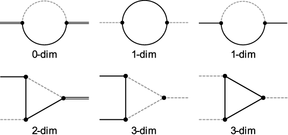
    As an example we present our results for two typical “building blocks”.

    • –

      The bubble integral with two massive lines (see Fig. 4, second diagram of the first row) and with massless external legs can be written in the following form

      ∫dd​ki​πd2​1[m2−k2]a1​[m2−(k+p)2]a2=\displaystyle\int\frac{{\rm d}^{d}k}{i\pi^{\frac{d}{2}}}\frac{1}{[m^{2}-k^{2}]^{a_{1}}[m^{2}-(k+p)^{2}]^{a_{2}}}=
      12​π​i​∫−i​∞+i​∞d​z​(m2)d2−a1−a2−z(−p2)−z\displaystyle\qquad\frac{1}{2\pi i}\int_{-i\infty}^{+i\infty}{\rm d}z\,\frac{(m^{2})^{\frac{d}{2}-a_{1}-a_{2}-z}}{(-p^{2})^{-z}}
      ×Γ⁡(−z)​Γ​(a1+z)​Γ​(a2+z)​Γ​(a1+a2−d2+z)Γ⁡(a1)​Γ​(a2)​Γ​(a1+a2+2​z).\displaystyle\qquad\times\frac{\Gamma(-z)\Gamma(a_{1}+z)\Gamma(a_{2}+z)\Gamma(a_{1}+a_{2}-\frac{d}{2}+z)}{\Gamma(a_{1})\Gamma(a_{2})\Gamma(a_{1}+a_{2}+2z)}\,. (18)
    • –

      The triangle integral with two massive internal lines and one massive, one massless and one on-shell leg (see first diagram of second row in Fig. 4) is given by

      ∫dd​ki​πd2​1[m2−(k+p1)2]a1​[m2−(k+p1+p2)2]a2​[−k2]a3=\displaystyle\int\frac{{\rm d}^{d}k}{i\pi^{\frac{d}{2}}}\frac{1}{[m^{2}-(k+p_{1})^{2}]^{a_{1}}[m^{2}-(k+p_{1}+p_{2})^{2}]^{a_{2}}[-k^{2}]^{a_{3}}}=
      1(2​π​i)2​∫−i​∞+i​∞d​z1​d​z2​(m2)d2−a1−a2−a3−z1−z2(m2−p12)−z1​(−p22)−z2\displaystyle\qquad\frac{1}{(2\pi i)^{2}}\int_{-i\infty}^{+i\infty}{\rm d}z_{1}{\rm d}z_{2}\,\frac{(m^{2})^{\frac{d}{2}-a_{1}-a_{2}-a_{3}-z_{1}-z_{2}}}{(m^{2}-p_{1}^{2})^{-z_{1}}(-p_{2}^{2})^{-z_{2}}}
      ×Γ⁡(−z1)​Γ​(−z2)​Γ​(a2+z2)​Γ​(a3+z1)​Γ​(a1+z1+z2)Γ⁡(a1)​Γ​(a2)​Γ​(a3)​Γ​(d−a1−a2−a3)\displaystyle\qquad\times\frac{\Gamma(-z_{1})\Gamma(-z_{2})\Gamma(a_{2}+z_{2})\Gamma(a_{3}+z_{1})\Gamma(a_{1}+z_{1}+z_{2})}{\Gamma(a_{1})\Gamma(a_{2})\Gamma(a_{3})\Gamma(d-a_{1}-a_{2}-a_{3})}
      ×Γ⁡(d−a1−a2−2​a3−z1)​Γ​(a1+a2+a3−d2+z1+z2)Γ⁡(a1+a2+z1+2​z2).\displaystyle\qquad\times\frac{\Gamma(d-a_{1}-a_{2}-2a_{3}-z_{1})\Gamma(a_{1}+a_{2}+a_{3}-\frac{d}{2}+z_{1}+z_{2})}{\Gamma(a_{1}+a_{2}+z_{1}+2z_{2})}\,. (19)

    Note that the exponents in Eqs. (18) and (19) need not be integer but may also depend on ϵ\epsilon.

    Refer to caption
    Figure 4: Sample building blocks for the loop-by-loop approach with three different types of external legs: dashed or solid lines denote massless- or massive propagators of general momentum p2p^{2} respectively. Their general complex powers can depend on the dimensional regularization parameter ϵ\epsilon and Mellin-Barnes integration variable ziz_{i}. Double lines are on-shell with the condition p2=m2p^{2}=m^{2}. The dimension of the Mellin-Barnes integration is specified below the diagrams.
  • •

    Decompose integral into products of building blocks.
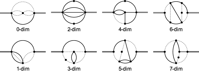
    The derived building blocks are applied step-by-step until all momentum integrations are replaced by Mellin-Barnes integrals. For simple integrals one ends up with a two- or three-dimensional integration (cf. Fig. 5). In theses cases a precision of about nine digits is achieved for the ϵ6\epsilon^{6} terms. The coefficients of the lower ϵ\epsilon-orders are more precise. We also encountered higher-dimensional integrals which lead to a lower precision. Some examples with five, six or even seven dimensional integrations can be found in Fig. 5. For these cases one obtains about five digits for the ϵ0\epsilon^{0} and two to three digits for the ϵ3\epsilon^{3} term.

    It is interesting to note that the decomposition into building blocks is not unique. In fact, different representations may have significantly different convergence properties which we exploited for some of the integrals.
Refer to caption
Figure 5: Sample master integrals which are treated with the Mellin-Barnes method. The dimension of the Mellin-Barnes integration is specified below the diagrams.

Altogether we have treated 80 master integrals with the help of the described method. The results of the Mellin-Barnes integrals are usually quite precise for lower orders of the ϵ\epsilon expansion and give several digits more than FIESTA provides. For 16 out of 80 integrals FIESTA produced more precise results for the higher orders in ϵ\epsilon and we chose to compose “hybrid” results where the lower orders were taken from the Mellin Barnes (MB) integrals and the ϵ3\epsilon^{3} or higher terms came from FIESTA.

For the preparation of the Mellin-Barnes integrals we use the package MB [68] together with its extensions discussed in Ref. [69]. For the numerical integration we use the integrator cuhre as implemented in the CUBA library [63]. As far as our experience goes the estimated uncertainty of cuhre is too small which can be seen by comparing the results of the numerical integration to (analytically) known results. Thus, we multiply the uncertainty by a factor 100 to be on the conservative side. For the higher-dimensional integrals we have also tried to use vegas, however, could not increase the precision [70].

We have compared all 80 master integrals computed with the Mellin-Barnes method with the FIESTA results and found good agreement for almost all ϵ\epsilon coefficients within three standard deviations. However, in a few cases deviations up to seven sigma are observed which once again justifies the use of a conservative limit of ten sigma for the Monte-Carlo uncertainty of FIESTA [70]. The systematic application of the Mellin-Barnes method is the main source for the improvements as compared to the results presented in Ref. [44].

The described procedure can, of course, only be applied to a subset of all master integrals. However, as mentioned above, in our basis these integrals provide the substantial part of the uncertainty to zmz_{m} in case we use the results based on FIESTA.

For the remaining 259 integrals (i.e. the ones which are neither known analytically nor treated with the Mellin-Barnes method) we use the FIESTA result. When inserting the master integrals we keep track of all uncertainties and combine them in quadrature in the final expression. We interpret the resulting uncertainty as a standard deviation and multiply it by ten (as justified above) in the final result for the relation between the MS¯\overline{\rm MS} and on-shell quark mass. Note that, if we add the uncertainties from the individual contributions linearly we obtain an uncertainty which is about five times larger than the uncertainty resulting from the quadratic combination. For example, zm(4)z_{m}^{(4)} for Nc=3N_{c}=3 and nl=5n_{l}=5 reads −871.732±0.180-871.732\pm 0.180 for quadratic and −871.732±0.872-871.732\pm 0.872 for the linear combination (without security factor 10).

3 Results for the MS¯\overline{\rm MS}-on-shell relation

As an outcome of the procedure discussed in the previous Section we obtain bare four-loop results for ΣV​(q2=Mq2)+ΣS​(q2=Mq2)\Sigma_{V}(q^{2}=M_{q}^{2})+\Sigma_{S}(q^{2}=M_{q}^{2}) which still contain fourth-order poles in the regularization parameter ϵ\epsilon. Furthermore, uncertainties from each ϵ\epsilon order of the numerically evaluated master integrals are present in the expression. The individual uncertainties shall eventually be combined quadratically to obtain the overall uncertainty. It is obvious that the latter is sensitive to the following choices:

  • •

    Set Nc=3N_{c}=3 (and optionally also a value for nln_{l}) before combining the uncertainties from the master integrals.

  • •

    Parametrize ΣV+ΣS\Sigma_{V}+\Sigma_{S} in terms of generic NcN_{c} and nln_{l}.

  • •

    Parametrize ΣV+ΣS\Sigma_{V}+\Sigma_{S} in terms of SU(Nc)(N_{c}) Casimir invariants.

In this Section we will discuss the three options. Note that we interpret the final uncertainty as a standard deviation which we multiply by a factor ten to be on the conservative side.

It is convenient to present results for the finite relation between the MS¯\overline{\rm MS} and on-shell mass. It is obtained after renormalization of the quark mass in the on-shell and the strong coupling constant in the MS¯\overline{\rm MS} scheme using three-loop renormalization constants. Whereas αs\alpha_{s} is renormalized by a simple multiplicative factor it is convenient to generate the mass counterterm contribution at the same time as the lower-order contributions. A finite quantity is obtained after dividing the (parameter renormalized) ZmOSZ_{m}^{\rm OS} by ZmMS¯Z_{m}^{\overline{\rm MS}}, as discussed around Eq. (10).

To get a sense of the quality of the cancellations of the poles we present in the following table results for three typical contributions to zm(4)z_{m}^{(4)} (μ2=M2\mu^{2}=M^{2})

zm(4)z_{m}^{(4)} for Nc=3N_{c}=3, nl=5n_{l}=5 coef. of Nc4N_{c}^{4} term coef. of CF4C_{F}^{4} term ϵ−4\epsilon^{-4} −0.00001-0.00001 ±\pm 0.000020.00002 −0.0000002-0.0000002 ±\pm 0.00000020.0000002 −0.000006-0.000006 ±\pm 0.0000130.000013 ϵ−3\epsilon^{-3} 0.00030.0003 ±\pm 0.00020.0002 0.0000020.000002 ±\pm 0.0000020.000002 0.00010.0001 ±\pm 0.00010.0001 ϵ−2\epsilon^{-2} −0.0002-0.0002 ±\pm 0.00180.0018 0.0000010.000001 ±\pm 0.0000160.000016 −0.0007-0.0007 ±\pm 0.00090.0009 ϵ−1\epsilon^{-1} 0.00440.0044 ±\pm 0.01910.0191 0.000020.00002 ±\pm 0.000180.00018 0.00050.0005 ±\pm 0.00810.0081 ϵ0\epsilon^{0} −871.732-871.732 ±\pm 0.1800.180 −51.181-51.181 ±\pm 0.0020.002 −6.983-6.983 ±\pm 0.0810.081


Note that the uncertainties are the ones returned from the numerical integration without introducing any security factor. Still, all pole coefficients are zero within one standard deviation which shows that the factor ten applied to the final results presented below is conservative.

From now on we only consider ϵ0\epsilon^{0} terms and choose μ2=M2\mu^{2}=M^{2} (for zmz_{m}) or μ2=m2​(μ2)\mu^{2}=m^{2}(\mu^{2}) (for cmc_{m}). The renormalization scale dependent terms can be computed analytically using renormalization group techniques; they are given in Appendix C.

3.1 Results for Nc=3N_{c}=3

We start with specifying both NcN_{c} and nln_{l} before combining the uncertainties of the master integrals. The results for zm(4)​(M)z_{m}^{(4)}(M) and cm(4)​(m)c_{m}^{(4)}(m) for Nc=3N_{c}=3 are shown in Table 1. Note that for the physically interesting cases nl=4,5n_{l}=4,5 and 66 we find a relative uncertainty between 0.1% and 0.2%.

nln_{l} zm(4)​(M)z_{m}^{(4)}(M) cm(4)​(m)c_{m}^{(4)}(m)
0 −3654.15-3654.15 ±\pm 1.641.64 3567.603567.60 ±\pm 1.641.64
1 −2940.01-2940.01 ±\pm 1.671.67 2864.602864.60 ±\pm 1.671.67
2 −2308.77-2308.77 ±\pm 1.701.70 2244.322244.32 ±\pm 1.701.70
3 −1756.36-1756.36 ±\pm 1.741.74 1702.701702.70 ±\pm 1.741.74
4 −1278.70-1278.70 ±\pm 1.771.77 1235.661235.66 ±\pm 1.771.77
5 −871.73-871.73 ±\pm 1.801.80 839.14839.14 ±\pm 1.801.80
6 −531.39-531.39 ±\pm 1.841.84 509.07509.07 ±\pm 1.841.84
7 −253.59-253.59 ±\pm 1.871.87 241.37241.37 ±\pm 1.871.87
8 −34.28-34.28 ±\pm 1.911.91 31.9931.99 ±\pm 1.911.91
9 130.62130.62 ±\pm 1.941.94 −123.15-123.15 ±\pm 1.941.94
10 245.17245.17 ±\pm 1.981.98 −228.12-228.12 ±\pm 1.981.98
11 313.45313.45 ±\pm 2.012.01 −286.98-286.98 ±\pm 2.012.01
12 339.51339.51 ±\pm 2.052.05 −303.81-303.81 ±\pm 2.052.05
13 327.44327.44 ±\pm 2.082.08 −282.68-282.68 ±\pm 2.082.08
14 281.30281.30 ±\pm 2.122.12 −227.64-227.64 ±\pm 2.122.12
15 205.16205.16 ±\pm 2.162.16 −142.78-142.78 ±\pm 2.162.16
16 103.09103.09 ±\pm 2.192.19 −32.15-32.15 ±\pm 2.192.19
17 −20.85-20.85 ±\pm 2.232.23 100.16100.16 ±\pm 2.232.23
18 −162.58-162.58 ±\pm 2.262.26 250.10250.10 ±\pm 2.262.26
19 −318.03-318.03 ±\pm 2.302.30 413.59413.59 ±\pm 2.302.30
20 −483.15-483.15 ±\pm 2.342.34 586.56586.56 ±\pm 2.342.34
Table 1: Results for zm(4)​(M)z_{m}^{(4)}(M) and cm(4)​(m)c_{m}^{(4)}(m) for Nc=3N_{c}=3 and 0≤nl≤200\leq n_{l}\leq 20.

From Table 1 one observes that the uncertainty has only a very mild dependence on nln_{l}. Thus, to a good approximation we can write zm(4)z_{m}^{(4)} in the form66 6 Note, that this is not a fit to Table 1.

zm(4)\displaystyle z_{m}^{(4)} =\displaystyle= −3654.15±1.64+(756.942±0.040)​nl−43.4824​nl2+0.678141​nl3.\displaystyle-3654.15\pm 1.64+(756.942\pm 0.040)n_{l}-43.4824n_{l}^{2}+0.678141n_{l}^{3}\,. (20)

In Fig. 6 we plot Eq. (20) for nln_{l} between 0 and 20 and combine the data points for integer nln_{l} to guide the eye. It is interesting to note that the four-loop coefficient zm(4)z_{m}^{(4)} becomes positive between nl=9n_{l}=9 and nl=16n_{l}=16. Close to these values of nln_{l} (i.e. for nl=8n_{l}=8 and nl=17n_{l}=17) the absolute value of zm(4)z_{m}^{(4)} is quite small and thus the relative uncertainty exceeds 5%. The range for nln_{l} where the four-loop coefficient changes sign coincides with the one for the so-called Banks-Zaks fixed point for the QCD beta function [71]. However, we are not aware of a deeper connection which might be a subject for further studies.

The four-loop coefficient of the inverted relation, cm(4)c_{m}^{(4)}, which is basically obtained from negative zm(4)z_{m}^{(4)} plus some products of lower order contributions, shows a similar behaviour except for the overall sign. It has, in particular, the same uncertainty, as can be seen in the last column of Table 1. The explicit nln_{l} dependence reads

cm(4)\displaystyle c_{m}^{(4)} =\displaystyle= 3567.60±1.64−(745.721±0.040)​nl+43.3963​nl2−0.678141​nl3.\displaystyle 3567.60\pm 1.64-(745.721\pm 0.040)n_{l}+43.3963n_{l}^{2}-0.678141n_{l}^{3}\,. (21)
Refer to caption
Figure 6: nln_{l}-dependence of zm(4)​(M)z_{m}^{(4)}(M).

For some applications it is useful to have control over all fermionic contributions, including the ones from closed fermion loops of mass MM which we label by nhn_{h}. The corresponding result is shown in Table 2 where we present the coefficients of nli​nhjn_{l}^{i}n_{h}^{j} for i,j=0,1,2,3i,j=0,1,2,3 with i+j≤3i+j\leq 3.

nl0​nh0n_{l}^{0}n_{h}^{0} −3678.28-3678.28 ±\pm 1.631.63
nl0​nh1n_{l}^{0}n_{h}^{1} 23.6323.63 ±\pm 0.120.12
nl0​nh2n_{l}^{0}n_{h}^{2} 0.52730.5273 ±\pm 0.00270.0027
nl0​nh3n_{l}^{0}n_{h}^{3} −0.02484-0.02484 ±\pm 0.000000.00000
nl1​nh0n_{l}^{1}n_{h}^{0} 757.64757.64 ±\pm 0.040.04
nl1​nh1n_{l}^{1}n_{h}^{1} −0.6646-0.6646 ±\pm 0.00040.0004
nl1​nh2n_{l}^{1}n_{h}^{2} −0.03617-0.03617 ±\pm 0.000000.00000
nl2​nh0n_{l}^{2}n_{h}^{0} −43.47-43.47 ±\pm 0.000.00
nl2​nh1n_{l}^{2}n_{h}^{1} −0.01720-0.01720 ±\pm 0.000000.00000
nl3​nh0n_{l}^{3}n_{h}^{0} 0.67810.6781 ±\pm 0.00000.0000
Table 2: zm(4)z_{m}^{(4)} decomposed into coefficients of nli​nhjn_{l}^{i}n_{h}^{j}.

3.2 Results for generic NcN_{c}

In a next step we do not specify numerical values for NcN_{c} and nln_{l} which leads to 23 non-zero colour structures. For the corresponding coefficients we obtain

zmL​L​L​1/Nc1\displaystyle z_{m}^{LLL1/N_{c}^{1}} =\displaystyle= −0.25430,\displaystyle-0.25430\,,
zmL​L​L​Nc1\displaystyle z_{m}^{LLLN_{c}^{1}} =\displaystyle= 0.25430,\displaystyle 0.25430\,,
zmL​L​1/Nc2\displaystyle z_{m}^{LL1/N_{c}^{2}} =\displaystyle= −0.14090,\displaystyle-0.14090\,,
zmL​L​1/Nc1\displaystyle z_{m}^{LL1/N_{c}^{1}} =\displaystyle= 0.00645,\displaystyle 0.00645\,,
zmL​L​Nc0\displaystyle z_{m}^{LLN_{c}^{0}} =\displaystyle= 5.58971,\displaystyle 5.58971\,,
zmL​L​Nc1\displaystyle z_{m}^{LLN_{c}^{1}} =\displaystyle= −0.00645,\displaystyle-0.00645\,,
zmL​L​Nc2\displaystyle z_{m}^{LLN_{c}^{2}} =\displaystyle= −5.44881,\displaystyle-5.44881\,,
zmL​1/Nc3\displaystyle z_{m}^{L1/N_{c}^{3}} =\displaystyle= 0.1788±0.0333,\displaystyle 0.1788\pm 0.0333\,,
zmL​1/Nc2\displaystyle z_{m}^{L1/N_{c}^{2}} =\displaystyle= −0.18076±0.00000,\displaystyle-0.18076\pm 0.00000\,,
zmL​1/Nc1\displaystyle z_{m}^{L1/N_{c}^{1}} =\displaystyle= 0.9282±0.0445,\displaystyle 0.9282\pm 0.0445\,,
zmL​Nc0\displaystyle z_{m}^{LN_{c}^{0}} =\displaystyle= 0.28392±0.00005,\displaystyle 0.28392\pm 0.00005\,,
zmL​Nc1\displaystyle z_{m}^{LN_{c}^{1}} =\displaystyle= −32.7991±0.0109,\displaystyle-32.7991\pm 0.0109\,,
zmL​Nc2\displaystyle z_{m}^{LN_{c}^{2}} =\displaystyle= −0.10316±0.00005,\displaystyle-0.10316\pm 0.00005\,,
zmL​Nc3\displaystyle z_{m}^{LN_{c}^{3}} =\displaystyle= 31.69215±0.00124,\displaystyle 31.69215\pm 0.00124\,,
zm1/Nc4\displaystyle z_{m}^{1/N_{c}^{4}} =\displaystyle= −0.4364±0.0503,\displaystyle-0.4364\pm 0.0503\,,
zm1/Nc3\displaystyle z_{m}^{1/N_{c}^{3}} =\displaystyle= 0.821±0.121,\displaystyle 0.821\pm 0.121\,,
zm1/Nc2\displaystyle z_{m}^{1/N_{c}^{2}} =\displaystyle= 0.1739±0.0738,\displaystyle 0.1739\pm 0.0738\,,
zm1/Nc1\displaystyle z_{m}^{1/N_{c}^{1}} =\displaystyle= 0.645±0.161,\displaystyle 0.645\pm 0.161\,,
zmNc0\displaystyle z_{m}^{N_{c}^{0}} =\displaystyle= −0.614±0.175,\displaystyle-0.614\pm 0.175\,,
zmNc1\displaystyle z_{m}^{N_{c}^{1}} =\displaystyle= −2.6228±0.0415,\displaystyle-2.6228\pm 0.0415\,,
zmNc2\displaystyle z_{m}^{N_{c}^{2}} =\displaystyle= 52.0579±0.0808,\displaystyle 52.0579\pm 0.0808\,,
zmNc3\displaystyle z_{m}^{N_{c}^{3}} =\displaystyle= 1.15654±0.00424,\displaystyle 1.15654\pm 0.00424\,,
zmNc4\displaystyle z_{m}^{N_{c}^{4}} =\displaystyle= −51.1812±0.0161,\displaystyle-51.1812\pm 0.0161\,, (22)

where the notation used for the superscripts is self-explanatory.77 7 Example: zmL​1/Nc2z_{m}^{L1/N_{c}^{2}} is the coefficient of nl/Nc2n_{l}/N_{c}^{2}; “LL” counts the factors nln_{l}. The nl3n_{l}^{3} and nl2n_{l}^{2} terms are known analytically and can be found in Ref. [72, 67] (see Appendix E). Both for the linear-nln_{l} and the nln_{l}-independent contribution one obtains small (relative) uncertainties for the positive powers in NcN_{c} which dominate in the physical limit Nc=3N_{c}=3. This explains the small uncertainties of coefficients in the previous subsection.

From Eq. (22) one learns that for Nc=3N_{c}=3 the dominant uncertainty originates from zmNc2z_{m}^{N_{c}^{2}}, followed by the NcN_{c}-independent term zmNc0z_{m}^{N_{c}^{0}}.

As a cross check we choose Nc=3N_{c}=3, fix nln_{l} and use the coefficients of Eqs. (22) to compute zm(4)z_{m}^{(4)} combining all uncertainties again quadratically. We obtain the following results

nln_{l} zm(4)z_{m}^{(4)}
3 −1756.36±1.52-1756.36\pm 1.52
4 −1278.70±1.53-1278.70\pm 1.53
5 −871.73±1.53-871.73\pm 1.53

The central values are by construction identical to the corresponding entries in Table 1, the uncertainties are even slightly smaller. This might happen since the uncertainties are added linearly when setting NcN_{c} and nln_{l} to numerical values before combining the uncertainties from the individual ϵ\epsilon terms (cf. Subsection 3.1). As compared to adding the uncertainties in quadrature this might lead to larger (as in the case at hand) or smaller (see next subsection) uncertainties.

3.3 Results in terms of Casimir colour factors

This subsection is devoted to the most general results, namely zmz_{m} in the form of Eq. (15). For the coefficients of the 23 colour structures we obtain

zmF​F​F​F\displaystyle z_{m}^{FFFF} =\displaystyle= −6.983±0.805,\displaystyle-6.983\pm 0.805\,,
zmF​F​F​A\displaystyle z_{m}^{FFFA} =\displaystyle= 13.40±2.07,\displaystyle 13.40\pm 2.07\,,
zmF​F​A​A\displaystyle z_{m}^{FFAA} =\displaystyle= −11.17±1.74,\displaystyle-11.17\pm 1.74\,,
zmF​A​A​A\displaystyle z_{m}^{FAAA} =\displaystyle= −99.272±0.493,\displaystyle-99.272\pm 0.493\,,
zmdF​A\displaystyle z_{m}^{d_{FA}} =\displaystyle= 0.39±1.07,\displaystyle 0.39\pm 1.07\,,
zmdF​F​L\displaystyle z_{m}^{d_{FF}L} =\displaystyle= −0.937±0.178,\displaystyle-0.937\pm 0.178\,,
zmdF​F​H\displaystyle z_{m}^{d_{FF}H} =\displaystyle= −3.924±0.642,\displaystyle-3.924\pm 0.642\,,
zmF​F​F​L\displaystyle z_{m}^{FFFL} =\displaystyle= −0.05094±0.00298,\displaystyle-0.05094\pm 0.00298\,,
zmF​F​A​L\displaystyle z_{m}^{FFAL} =\displaystyle= 9.26642±0.00454,\displaystyle 9.26642\pm 0.00454\,,
zmF​A​A​L\displaystyle z_{m}^{FAAL} =\displaystyle= 122.1872±0.0100,\displaystyle 122.1872\pm 0.0100\,,
zmF​F​L​L\displaystyle z_{m}^{FFLL} =\displaystyle= −2.25441,\displaystyle-2.25441\,,
zmF​A​L​L\displaystyle z_{m}^{FALL} =\displaystyle= −42.46326,\displaystyle-42.46326\,,
zmF​L​L​L\displaystyle z_{m}^{FLLL} =\displaystyle= 4.06885,\displaystyle 4.06885\,,
zmF​F​F​H\displaystyle z_{m}^{FFFH} =\displaystyle= −1.3625±0.0132,\displaystyle-1.3625\pm 0.0132\,,
zmF​F​A​H\displaystyle z_{m}^{FFAH} =\displaystyle= 14.9800±0.0334,\displaystyle 14.9800\pm 0.0334\,,
zmF​A​A​H\displaystyle z_{m}^{FAAH} =\displaystyle= −2.3597±0.0342,\displaystyle-2.3597\pm 0.0342\,,
zmF​F​H​H\displaystyle z_{m}^{FFHH} =\displaystyle= 1.65752±0.00031,\displaystyle 1.65752\pm 0.00031\,,
zmF​A​H​H\displaystyle z_{m}^{FAHH} =\displaystyle= −0.20934±0.00273,\displaystyle-0.20934\pm 0.00273\,,
zmF​H​H​H\displaystyle z_{m}^{FHHH} =\displaystyle= −0.14902±0.00000,\displaystyle-0.14902\pm 0.00000\,,
zmF​F​L​H\displaystyle z_{m}^{FFLH} =\displaystyle= −2.89209±0.00010,\displaystyle-2.89209\pm 0.00010\,,
zmF​A​L​H\displaystyle z_{m}^{FALH} =\displaystyle= 0.62076±0.00042,\displaystyle 0.62076\pm 0.00042\,,
zmF​L​L​H\displaystyle z_{m}^{FLLH} =\displaystyle= −0.10321,\displaystyle-0.10321\,,
zmF​L​H​H\displaystyle z_{m}^{FLHH} =\displaystyle= −0.21703±0.00000.\displaystyle-0.21703\pm 0.00000\,. (23)

The nl3n_{l}^{3} and nl2n_{l}^{2} terms are known analytically and can be found in Appendix E. The linear-nln_{l} term is dominated by zmF​A​A​Lz_{m}^{FAAL} which has an uncertainty below 0.01%. On the other hand, for zmF​F​F​Lz_{m}^{FFFL} the precision is only about 4%, however, the numerical impact is small, even for Nc=2N_{c}=2.

The contributions involving closed heavy quark loops are generally small and known to a precision of about 10% or better, the numerically dominant zmF​F​A​Hz_{m}^{FFAH} contribution even to about 1.3%.

There are five non-fermionic contributions, zmF​F​F​Fz_{m}^{FFFF}, zmF​F​F​Az_{m}^{FFFA}, zmF​F​A​Az_{m}^{FFAA}, zmF​A​A​Az_{m}^{FAAA} and zmdF​Az_{m}^{d_{FA}}. The most precise one, zmF​A​A​Az_{m}^{FAAA}, has by far the largest coefficient and furthermore the largest colour factor. The three coefficients zmF​F​F​Fz_{m}^{FFFF}, zmF​F​F​Az_{m}^{FFFA} and zmF​F​A​Az_{m}^{FFAA} have an uncertainty between 11% and 15%. zmdF​Az_{m}^{d_{FA}} is the worst known coefficient. Actually, within our precision we cannot claim whether it is positive or negative. Note, however, that not only the coefficient itself but also the colour factor is numerically small as compared to others. For example, for Nc=3N_{c}=3 we have dFa​b​c​d​dAa​b​c​d/Nc=15/6=2.5d^{abcd}_{F}d^{abcd}_{A}/N_{c}=15/6=2.5 whereas CF​CA3=36C_{F}C_{A}^{3}=36. The current uncertainty of zmdF​Az_{m}^{d_{FA}} is dominated by master integrals where we rely on the FIESTA results.

As a cross check we insert the results from Eq. (23) into Eq. (15) and specify the colour factors to their numerical values with Nc=3N_{c}=3. We add all uncertainties in quadrature and obtain

nln_{l} zm(4)z_{m}^{(4)}
3 −1756.36±36.3-1756.36\pm 36.3
4 −1278.70±36.3-1278.70\pm 36.3
5 −871.73±36.3-871.73\pm 36.3

which has to be compared with the corresponding entries in Table 1 where Nc=3N_{c}=3 is chosen before combining the uncertainties from the individual master integrals. As expected, one observes the same central value, however, the uncertainties are significantly larger.

4 Applications

4.1 MS¯\overline{\rm MS}-on-shell transformation formulae

In the following we discuss the relation between the MS¯\overline{\rm MS} and on-shell quark mass and specify the number of massless quarks to the top, bottom and charm case.

Let us start with the version where the on-shell mass is computed from the MS¯\overline{\rm MS} mass. We use as input the following MS¯\overline{\rm MS} masses

mt​(mt)\displaystyle m_{t}(m_{t}) =\displaystyle= 163.508​GeV,\displaystyle 163.508~\mbox{GeV}\,,
mb​(mb)\displaystyle m_{b}(m_{b}) =\displaystyle= 4.163​GeV,\displaystyle 4.163~\mbox{GeV}\,,
mc​(3​GeV)\displaystyle m_{c}(3~\mbox{GeV}) =\displaystyle= 0.986​GeV,\displaystyle 0.986~\mbox{GeV}\,, (24)

where mt​(mt)m_{t}(m_{t}) is computed from Mt=173.34M_{t}=173.34 GeV [10] using four-loop accuracy. The MS¯\overline{\rm MS} masses for charm and bottom are taken from Ref. [3].

The values for the strong coupling are given by αs(6)​(mt)=0.1085\alpha_{s}^{(6)}(m_{t})=0.1085, αs(5)​(mb)=0.2253\alpha_{s}^{(5)}(m_{b})=0.2253, and αs(4)​(3​GeV)=0.2540\alpha_{s}^{(4)}(3~\mbox{GeV})=0.2540. They have been computed from αs(5)​(MZ)=0.1181\alpha_{s}^{(5)}(M_{Z})=0.1181 using RunDec [46, 47]. In the case of the charm quark we also provide results for μ=mc​(mc)\mu=m_{c}(m_{c}) using the input values mc​(mc)=1.279m_{c}(m_{c})=1.279 GeV and αs(4)​(mc)=0.3872\alpha_{s}^{(4)}(m_{c})=0.3872. Note that the choice μ=3\mu=3 GeV is preferable since it has the advantage that low renormalization scales μ≈mc\mu\approx m_{c} are avoided.

In the following equations we list the results for the relations which convert the MS¯\overline{\rm MS} to the on-shell mass. For simplicity we set here and in the remainder of this section the uncertainty of the four-loop coefficient to 0.2% although it is for charm and bottom slightly smaller (see Table 1). We obtain

Mt\displaystyle M_{t} =\displaystyle= mt​(mt)​(1+0.4244​αs+0.8345​αs2+2.375​αs3+(8.615±0.017)​αs4)\displaystyle m_{t}(m_{t})\left(1+0.4244\,{\alpha_{s}}+0.8345\,{\alpha_{s}^{2}}+2.375\,{\alpha_{s}^{3}}+(8.615\pm 0.017)\,{\alpha_{s}^{4}}\right) (25)
=\displaystyle= ​163.508+7.529+1.606+0.496+(0.195±0.0004)​GeV,\displaystyle\mbox{}163.508+7.529+1.606+0.496+(0.195\pm 0.0004)~\mbox{GeV}\,,
Mb\displaystyle M_{b} =\displaystyle= mb​(mb)​(1+0.4244​αs+0.9401​αs2+3.045​αs3+(12.685±0.025)​αs4)\displaystyle m_{b}(m_{b})\left(1+0.4244\,{\alpha_{s}}+0.9401\,{\alpha_{s}^{2}}+3.045\,{\alpha_{s}^{3}}+(12.685\pm 0.025)\,{\alpha_{s}^{4}}\right) (26)
=\displaystyle= ​4.163+0.398+0.199+0.145+(0.136±0.0003)​GeV,\displaystyle\mbox{}4.163+0.398+0.199+0.145+(0.136\pm 0.0003)~\mbox{GeV}\,,
Mc\displaystyle M_{c} =\displaystyle= mc​(3​GeV)​(1+1.133​αs+3.119​αs2+10.981​αs3+(51.419±0.102)​αs4)\displaystyle m_{c}(3~\mbox{GeV})\left(1+1.133\,{\alpha_{s}}+3.119\,{\alpha_{s}^{2}}+10.981\,{\alpha_{s}^{3}}+(51.419\pm 0.102)\,{\alpha_{s}^{4}}\right) (27)
=\displaystyle= ​0.986+0.284+0.198+0.177+(0.211±0.0004)​GeV,\displaystyle\mbox{}0.986+0.284+0.198+0.177+(0.211\pm 0.0004)~\mbox{GeV}\,,
Mc\displaystyle M_{c} =\displaystyle= mc​(mc)​(1+0.4244​αs+1.0456​αs2+3.757​αs3+(17.480±0.035)​αs4)\displaystyle m_{c}(m_{c})\left(1+0.4244\,{\alpha_{s}}+1.0456\,{\alpha_{s}^{2}}+3.757\,{\alpha_{s}^{3}}+(17.480\pm 0.035)\,{\alpha_{s}^{4}}\right) (28)
=\displaystyle= ​1.279+0.210+0.200+0.279+(0.503±0.001)​GeV,\displaystyle\mbox{}1.279+0.210+0.200+0.279+(0.503\pm 0.001)~\mbox{GeV}\,,

where the renormalization scale of αs\alpha_{s} in each equation is identical to the one specified for the MS¯\overline{\rm MS} quark mass in the prefactor of the first lines in each equation.

One observes a good convergence for the top quark where the coefficients steadily decrease; the four-loop coefficient is more than a factor two smaller than the three-loop one. This is different for charm and bottom where the two-, three- and four-loop coefficients are of the same order of magnitude. In Eq. (28) (where μ2=mc2\mu^{2}=m_{c}^{2} has been chosen) the four-loop coefficient is even almost twice as large as the three-loop coefficient.

For convenience we also present the inverted relation of Eq. (25) which is given by

mt​(mt)\displaystyle m_{t}(m_{t}) =\displaystyle= Mt​(1−0.4244​αs−0.9246​αs2−2.593​αs3−(8.949±0.018)​αs4)\displaystyle M_{t}\left(1-0.4244\,{\alpha_{s}}-0.9246\,{\alpha_{s}^{2}}-2.593\,{\alpha_{s}^{3}}-(8.949\pm 0.018)\,{\alpha_{s}^{4}}\right) (29)
=\displaystyle= ​173.34−7.924−1.859−0.562−(0.209±0.0004)​GeV,\displaystyle\mbox{}173.34-7.924-1.859-0.562-(0.209\pm 0.0004)~\mbox{GeV}\,,

where αs≡αs​(Mt)=0.1077\alpha_{s}\equiv\alpha_{s}(M_{t})=0.1077. We refrain from providing the analogue equations for charm and bottom since this would require specifying the pole masses.

4.2 Relation between MS¯\overline{\rm MS} and threshold mass

The threshold masses are constructed such that the relation to the MS¯\overline{\rm MS} mass is well behaved in perturbation theory. It is illustrating to examine the cancellations which take place between the coefficients in the MS¯\overline{\rm MS}-OS relation and the ones in the relation of the OS and threshold mass. For example, in the case for the bottom quark mass we have for the PS mass

mbPS​(μf=2​GeV)\displaystyle m_{b}^{\rm PS}(\mu_{f}=2~\mbox{GeV}) =\displaystyle= 4.163+(0.399−0.191)+(0.199−0.120)\displaystyle 4.163+(0.399-0.191)+(0.199-0.120) (30)
+(0.145−0.114)+(0.1364−0.1368±0.0003)​GeV\displaystyle+(0.145-0.114)+(0.1364-0.1368\pm 0.0003)~\mbox{GeV}
=\displaystyle= 4.163+0.207+0.080+0.032−(0.0004±0.0003)​GeV,\displaystyle 4.163+0.207+0.080+0.032-(0.0004\pm 0.0003)~\mbox{GeV}\,,

where the second terms inside the round brackets after the first equality sign originate from the PS-OS relation. As expected due to the very definition of the PS mass, one observes a significant cancellation between the coefficients of the PS-OS and PS-MS¯\overline{\rm MS} relation. The cancellation becomes stronger at higher loop-order. In particular, at four loops one observes a cancellation of three significant digits, which is the reason why four digits after the comma are provided. Note that the details of the cancellations depend on μf\mu_{f}, as we will discuss in Section 4.3.

After the second equality sign the numbers in the round brackets are added. One observes a nice convergence behaviour with decreasing coefficients which has to be compared to the OS-MS¯\overline{\rm MS} relation where the three- and four-loop coefficients have the same order of magnitude, cf. Eq. (26). The four-loop coefficient in Eq. (30) only amounts to −0.4-0.4 MeV which is actually of the same order of magnitude as the uncertainty. Note, however, that both the central value and the uncertainty are far below the expected precision of the MS¯\overline{\rm MS} bottom quark mass within the foreseeable future.

The analogue equation to (30) for the top quark reads

mtPS​(μf=80​GeV)\displaystyle m_{t}^{\rm PS}(\mu_{f}=80~\mbox{GeV}) =\displaystyle\!=\! 163.508+(7.531−3.685)+(1.607−0.989)\displaystyle 163.508+(7.531-3.685)+(1.607-0.989) (31)
+(0.495−0.403)+(0.195−0.211±0.0004)​GeV\displaystyle+(0.495-0.403)+(0.195-0.211\pm 0.0004)~\mbox{GeV}
=\displaystyle\!=\! 163.508+3.847+0.618+0.092−(0.016±0.0004)​GeV.\displaystyle 163.508+3.847+0.618+0.092-(0.016\pm 0.0004)~\mbox{GeV}\,.

Also here one observes a drastic reduction of the correction terms when going to higher orders. In fact, the last term amounts to only 16 MeV instead of 200 MeV in Eq. (25).

For the 1S mass we obtain the following perturbative relations to the MS¯\overline{\rm MS} bottom and top mass

mb1​S\displaystyle m_{b}^{\rm 1S} =\displaystyle= 4.163+(0.399−0.047)+(0.195−0.072)\displaystyle 4.163+(0.399-0.047)+(0.195-0.072)
+(0.139−0.100)+(0.129−0.137±0.0003)​GeV\displaystyle+(0.139-0.100)+(0.129-0.137\pm 0.0003)~\mbox{GeV}
=\displaystyle= 4.163+0.352+0.123+0.039−(0.008±0.0003)​GeV,\displaystyle 4.163+0.352+0.123+0.039-(0.008\pm 0.0003)~\mbox{GeV}\,,
mt1​S\displaystyle m_{t}^{\rm 1S} =\displaystyle= 163.508+(7.531−0.428)+(1.588−0.368)\displaystyle 163.508+(7.531-0.428)+(1.588-0.368) (32)
+(0.479−0.262)+(0.185−0.174±0.0004)​GeV\displaystyle+(0.479-0.262)+(0.185-0.174\pm 0.0004)~\mbox{GeV}
=\displaystyle= 163.508+7.103+1.220+0.217+(0.011±0.0004)​GeV,\displaystyle 163.508+7.103+1.220+0.217+(0.011\pm 0.0004)~\mbox{GeV}\,,

where the first and second number in the bracket originates from the OS-MS¯\overline{\rm MS} and OS-1S relation, respectively. Furthermore, we order the terms according the ε\varepsilon expansion as defined in Refs. [5, 6, 7]. It is interesting to note that at leading order (LO) (first round bracket) the contribution from the OS-1S relation amounts only to a few per cent of the OS-MS¯\overline{\rm MS} relation. At N3LO, however, it is more than 90% both for bottom and top.

Similar results to those presented in Eqs. (30), (31) and (32) for bottom and top are also obtained for the charm quark in case μ=3\mu=3 GeV is chosen for the renormalization scale. On the other hand, in the case when the relation of the threshold mass to mc​(mc)m_{c}(m_{c}) is computed the four-loop term exceeds the three-loop one. We furthermore observe that the relations to the RS and RS′ masses behave very similar to the PS and 1S masses. We refrain from providing explicit results which are easily obtained with the help of RunDec [46] and CRunDec [47].

In practice a threshold quark mass is extracted from comparison of experimental measurements and theory predictions. Afterwards it is converted to the MS¯\overline{\rm MS} quark mass. In Table 3 we show the results for the scale invariant MS¯\overline{\rm MS} quark masses mq​(mq)m_{q}(m_{q}) (q=t,b,cq=t,b,c) and mc​(3​GeV)m_{c}(3~\mbox{GeV}) using one- to four-loop accuracy for the conversion. The input values for the threshold masses (which are provided at the top of each table) are chosen such that the four-loop results agree with the input values discussed in Eq. (24). For the top quark a rapid convergence is observed with four-loop contributions between 10 and 20 MeV. The situation is similar for the bottom quark where the four-loop term amounts to at most 8 MeV for the case of the 1S mass. As already mentioned above, the four-loop term for the case where mc​(mc)m_{c}(m_{c}) is computed from the threshold masses is larger than the three-loop contribution which is different for mc​(3​GeV)m_{c}(3~\mbox{GeV}) where the four-loop term is smaller by up to a factor four. Thus, even in this case we observe a reasonable convergence of the perturbative series; for the PS and RS masses the N3LO corrections are even below 10 MeV.

The results in Table 3 show that perturbatively well-behaved quark mass relations are obtained after introducing threshold masses. To exploit them at third order in perturbation theory, which is mandatory due to current precision reached for the quark masses, it is necessary to use the four-loop relation between the on-shell and MS¯\overline{\rm MS} quark mass for the construction of the MS¯\overline{\rm MS}-threshold mass relation.

input mPS=m^{\rm PS}= m1​S=m^{\rm 1S}= mRS=m^{\rm RS}= mRS′=m^{\rm RS^{\prime}}=
#loops 168.049 172.060 166.290 171.785
1 164.174 164.904 163.702 164.226
2 163.580 163.727 163.520 163.591
3 163.492 163.519 163.490 163.500
4 163.508 163.508 163.508 163.508
4 (×1.002\times 1.002) 163.507 163.507 163.507 163.507
input mPS=m^{\rm PS}= m1​S=m^{\rm 1S}= mRS=m^{\rm RS}= mRS′=m^{\rm RS^{\prime}}=
#loops 4.481 4.668 4.364 4.692
1 4.266 4.308 4.210 4.286
2 4.191 4.192 4.173 4.196
3 4.163 4.155 4.159 4.165
4 4.163 4.163 4.163 4.163
4 (×1.002\times 1.002) 4.163 4.163 4.163 4.163
(a) mt​(mt)m_{t}(m_{t}) (b) mb​(mb)m_{b}(m_{b})
input mPS=m^{\rm PS}= m1​S=m^{\rm 1S}= mRS=m^{\rm RS}= mRS′=m^{\rm RS^{\prime}}=
#loops 1.130 1.513 1.035 1.351
1 1.255 1.342 1.249 1.146
2 1.230 1.250 1.273 1.276
3 1.235 1.214 1.249 1.250
4 1.279 1.279 1.279 1.279
4 (×1.002\times 1.002) 1.278 1.278 1.278 1.278
input mPS=m^{\rm PS}= m1​S=m^{\rm 1S}= mRS=m^{\rm RS}= mRS′=m^{\rm RS^{\prime}}=
#loops 1.153 1.545 1.043 1.357
1 1.077 1.261 1.028 1.074
2 1.021 1.117 1.008 1.020
3 0.993 1.032 0.992 0.995
4 0.986 0.986 0.986 0.986
4 (×1.002\times 1.002) 0.986 0.986 0.986 0.986
(c) mc​(mc)m_{c}(m_{c}) (d) mc​(3​GeV)m_{c}(3~\mbox{GeV})
Table 3: mq​(mq)m_{q}(m_{q}) (q=t,b,cq=t,b,c) in GeV [see (a), (b), (c)] and mc​(3​GeV)m_{c}(3~\mbox{GeV}) (d) computed from the PS, 1S, RS and RS′ quark mass using LO to N3LO accuracy. The numbers in the last line are obtained by taking into account the uncertainty of the four-loop coefficient, i.e., it is increased by 0.2%. This leads to a shift of at most 1 MeV. The factorization scales for the PS, RS and RS′ masses are set to 2 GeV for bottom and charm. For the top quark we use μf=80\mu_{f}=80 GeV for the PS, RS and RS′ masses.
Refer to caption Refer to caption
(a) (b)
Refer to caption Refer to caption
(c) (d)
Refer to caption Refer to caption
(e) (f)
Figure 7: (a) MS¯\overline{\rm MS} top quark mass mt​(mt)m_{t}(m_{t}) computed from the PS mass with LO, NLO, NNLO and N3LO accuracy as a function of the renormalization scale used in the MS¯\overline{\rm MS}-threshold mass relation. (b) MS¯\overline{\rm MS} top quark mass mt​(mt)m_{t}(m_{t}) computed from the PS, 1S, RS and RS′ mass with NNLO (dashed) and N3LO (solid line) accuracy as a function of the renormalization scale used in the MS¯\overline{\rm MS}-threshold mass relation. At the right end of the plot the lines from bottom to top correspond to the RS, PS, RS′ 1S mass. (c)-(f) show the results for bottom and charm. For the bottom quark the four-loop result for the 1S mass is below (above) the others for high (low) values of μ\mu.

To obtain the results in Table 3 we have set the renormalization scale in the relation between the threshold and MS¯\overline{\rm MS} mass to the quark mass itself or to 3 GeV. As an alternative one could also apply the conversion relation at some intermediate scale μ\mu and then run with four-loop accuracy in the MS¯\overline{\rm MS} scheme for either the scale invariant mass or to μ=3\mu=3 GeV for the charm quark. The corresponding results are shown in Fig. 7 where mt​(mt)m_{t}(m_{t}), mb​(mb)m_{b}(m_{b}) and mc​(3​GeV)m_{c}(3~\mbox{GeV}) are shown as a function of the intermediate scale μ\mu. The panels on the left show the results for the PS mass for the one- to four-loop analysis. In all three cases one observes a rapid convergence when including higher order corrections resulting in an almost horizontal, i.e, μ\mu independent, result at four loops.

The panels on the right compare the various threshold masses at three and four loops. Note that by construction the four-loop curves coincide for μ=mq​(mq)\mu=m_{q}(m_{q}) for top and bottom and for μ=3\mu=3 GeV for charm. In all cases one observes that the four-loop curves are significantly flatter than the three-loop results. Particularly good results are obtained for the top quark in panel (b) where in a large range the four-loop results lie on top of each other. The four-loop curves in the case of the bottom quark show stronger variations below, say, μ=2.5\mu=2.5 GeV. Here the PS, RS and RS′ results are quite close together whereas the 1S curve shows a quite strong rise for μ→2\mu\to 2 GeV. Note that the scale on the yy axis for the charm plot covers a bigger range than for the bottom quark. Nevertheless the four-loop curve shows a quite flat behaviour. One observes again that the 1S curve deviates from the remaining ones.

4.3 μf\mu_{f} dependence of PS, RS and RS′ mass

Refer to caption Refer to caption
Figure 8: Three- (black, lower three curves in each plot) and four-loop (red, upper three curves in each plot) contribution in transition form PS, RS and RS′ mass to mq​(mq)m_{q}(m_{q}) and mc​(3​GeV)m_{c}(3~\mbox{GeV}) as a function of the factorization scale μf\mu_{f}.

In this Section we study the dependence of the PS, RS and RS′ mass on the factorization scale μf\mu_{f}. To do this we use mt​(mt)m_{t}(m_{t}), mb​(mb)m_{b}(m_{b}), mc​(mc)m_{c}(m_{c}) and mc​(3​GeV)m_{c}(3~\mbox{GeV}) from Eq. (24) and compute the threshold masses for the given value of μf\mu_{f} to four-loop accuracy. This value is then used as starting point for the computation of the MS¯\overline{\rm MS} mass at one- to four-loop order as a function of μf\mu_{f}. In Fig. 8 the three- (black) and four-loop (red) contributions to the conversion formula are plotted for the PS (solid), RS (short dashes) and RS′ (long dashes) masses. In the case of the top quark the default scale for the PS mass suggested in Ref. [4] is μf=20\mu_{f}=20 GeV. For this value the four-loop contribution amounts to about −50-50 MeV. One observes that the perturbative conversion formula is better behaved for larger values of μf\mu_{f}. In fact, the four-loop term vanishes for μf≈50\mu_{f}\approx 50 MeV and amounts to about +10+10 MeV for μf≈80\mu_{f}\approx 80 MeV, a value suggested in Ref. [14] in the context of top quark pair production close to threshold. Similar conclusions also hold for the RS and RS′ masses.

For the bottom quark the general behaviour of the three- and four-loop correction terms is similar to the top quark case. Here, the suggested default value of μf=2\mu_{f}=2 GeV [4, 8] seems to be a good choice from the perturbative point of view.

For completeness we show in Fig. 8 the corresponding results for the charm quark masses mc​(mc)m_{c}(m_{c}) and mc​(3​GeV)m_{c}(3~\mbox{GeV}). Here, the results are less conclusive, in particular for mc​(mc)m_{c}(m_{c}). Over a large range of μf\mu_{f} the four-loop term is even larger than the three-loop contribution which is a sign that the formalism should not be applied to mc​(mc)m_{c}(m_{c}). The situation is better in case mc​(3​GeV)m_{c}(3~\mbox{GeV}) is considered, which is probably due to the smaller values of αs\alpha_{s} (which increases significantly when going from μ=3\mu=3 GeV to μ=mc​(mc)≈1.3\mu=m_{c}(m_{c})\approx 1.3 GeV). For mc​(3​GeV)m_{c}(3~\mbox{GeV}) the four-loop contribution is always smaller than the three-loop term, however, it comes close to zero only for values near μf≈3\mu_{f}\approx 3 GeV.

4.4 cmc_{m} in terms of αs(nl)\alpha_{s}^{(n_{l})}

For certain applications (see, e.g, Ref. [2]) it is necessary to express the MS¯\overline{\rm MS}-on-shell relation in terms of αs(nl)\alpha_{s}^{(n_{l})} instead of αs(nl+1)\alpha_{s}^{(n_{l}+1)}. It is obtained by using the decoupling relation for αs\alpha_{s} which is given by88 8 The formulae of this subsection and the ones of the appendices (except Appendix E) can be found on the website https://www.ttp.kit.edu/_\_ media/progdata/2016/ttp16-023.tgz.

αs(nl+1)=ζαs​αs(nl),\alpha_{s}^{(n_{l}+1)}=\zeta_{\alpha_{s}}\alpha_{s}^{(n_{l})}\,, (33)

with

ζαs=1+16​αs(nl)π​log⁡(μ2m2​(μ2))+𝒪⁡(αs2),\zeta_{\alpha_{s}}=1+\frac{1}{6}\frac{\alpha_{s}^{(n_{l})}}{\pi}\log\left(\frac{\mu^{2}}{m^{2}(\mu^{2})}\right)+{\cal O}(\alpha_{s}^{2})\,, (34)

where results up to four-loop order can be found in Refs. [73, 74]. In our case we only need three-loop corrections which have been computed for the first time in Ref. [75]. Inserting Eq. (33) into the equation for zmz_{m} leads to

cm​(nl)=cm​(nl+1)|αs(nl+1)→αs(nl)+δ​cm​(nl),c_{m}(n_{l})=c_{m}(n_{l}+1)|_{\alpha_{s}^{(n_{l}+1)}\to\alpha_{s}^{(n_{l})}}+\delta c_{m}(n_{l})\,, (35)

with

δ​cm(2)=lμ26+2​lμ9,\displaystyle\delta c_{m}^{(2)}=\frac{l_{\mu}^{2}}{6}+\frac{2l_{\mu}}{9}\,, (36)
δcm(3)=[(−ζ318+π29+11732+127π2log(2))lμ+5​lμ38+25​lμ29\displaystyle\delta c_{m}^{(3)}=\bigg[\bigg(-\frac{\zeta_{3}}{18}+\frac{\pi^{2}}{9}+\frac{117}{32}+\frac{1}{27}\pi^{2}\log(2)\bigg)l_{\mu}+\frac{5l_{\mu}^{3}}{8}+\frac{25l_{\mu}^{2}}{9}
+{−lμ336−13​lμ2108+(−71432−π254)lμ}nl−1154],\displaystyle+\bigg\{-\frac{l_{\mu}^{3}}{36}-\frac{13l_{\mu}^{2}}{108}+\bigg(-\frac{71}{432}-\frac{\pi^{2}}{54}\bigg)l_{\mu}\bigg\}n_{l}-\frac{11}{54}\bigg]\,, (37)
δcm(4)=[lμ(−110​a427−1439​π2​ζ3864+107515​ζ327648+1975​ζ5432−695​π415552+676601​π277760\displaystyle\delta c_{m}^{(4)}=\bigg[l_{\mu}\bigg(-\frac{110a_{4}}{27}-\frac{1439\pi^{2}\zeta_{3}}{864}+\frac{107515\zeta_{3}}{27648}+\frac{1975\zeta_{5}}{432}-\frac{695\pi^{4}}{15552}+\frac{676601\pi^{2}}{77760}
OPEN+18532949373248−55​log4​(2)324−1181​π2​log2⁡(2)−271162​π2​log⁡(2))\displaystyle+\frac{18532949}{373248}-\frac{55\log^{4}(2)}{324}-\frac{11}{81}\pi^{2}\log^{2}(2)-\frac{271}{162}\pi^{2}\log(2)\bigg)
+nl{lμ(4​a427−241​ζ3144+61​π43888−1057​π21296−50214593312+log4⁡(2)162\displaystyle+n_{l}\bigg\{l_{\mu}\bigg(\frac{4a_{4}}{27}-\frac{241\zeta_{3}}{144}+\frac{61\pi^{4}}{3888}-\frac{1057\pi^{2}}{1296}-\frac{502145}{93312}+\frac{\log^{4}(2)}{162}
OPEN+181​π2​log2⁡(2)−11162​π2​log⁡(2))+(−7​ζ318−25​π2108−112332592−154​π2​log⁡(2))​lμ2\displaystyle+\frac{1}{81}\pi^{2}\log^{2}(2)-\frac{11}{162}\pi^{2}\log(2)\bigg)+\bigg(-\frac{7\zeta_{3}}{18}-\frac{25\pi^{2}}{108}-\frac{11233}{2592}-\frac{1}{54}\pi^{2}\log(2)\bigg)l_{\mu}^{2}
−83​lμ4432−1171​lμ3864+11​π2648+1229546656}+83099​ζ320736+(−17​ζ318+19​π218+44217710368\displaystyle-\frac{83l_{\mu}^{4}}{432}-\frac{1171l_{\mu}^{3}}{864}+\frac{11\pi^{2}}{648}+\frac{12295}{46656}\bigg\}+\frac{83099\zeta_{3}}{20736}+\bigg(-\frac{17\zeta_{3}}{18}+\frac{19\pi^{2}}{18}+\frac{442177}{10368}
+1954π2log(2))lμ2+431​lμ4216+8869​lμ3648+nl2{(7​ζ3108+13​π2648+235346656)lμ+lμ4216\displaystyle+\frac{19}{54}\pi^{2}\log(2)\bigg)l_{\mu}^{2}+\frac{431l_{\mu}^{4}}{216}+\frac{8869l_{\mu}^{3}}{648}+n_{l}^{2}\bigg\{\bigg(\frac{7\zeta_{3}}{108}+\frac{13\pi^{2}}{648}+\frac{2353}{46656}\bigg)l_{\mu}+\frac{l_{\mu}^{4}}{216}
+13​lμ3432+(891296+π2108)lμ2}−11​π2108−20956723328−11324π2log(2)],\displaystyle+\frac{13l_{\mu}^{3}}{432}+\bigg(\frac{89}{1296}+\frac{\pi^{2}}{108}\bigg)l_{\mu}^{2}\bigg\}-\frac{11\pi^{2}}{108}-\frac{209567}{23328}-\frac{11}{324}\pi^{2}\log(2)\bigg]\,, (38)

with

lμ=log⁡(μ2m2​(μ)),an=Lin​(12).l_{\mu}=\log\left(\frac{\mu^{2}}{{m^{2}(\mu)}}\right)\,,\quad a_{n}=\mathrm{Li}_{n}\left(\frac{1}{2}\right)\,. (39)

5 Conclusions

The main result of this paper is the calculation of the four-loop coefficient in the relation between the MS¯\overline{\rm MS} and on-shell heavy quark mass. Up to the reduction to master integrals the calculation is performed analytically. However, most of the master integrals are only known numerically. For QCD, we managed to obtain an uncertainty of 0.2% for the four-loop coefficient.

We have also computed the coefficients of the individual colour structures. It is interesting to note that the large coefficients (zmF​A​A​Az_{m}^{FAAA} and zmF​A​A​Lz_{m}^{FAAL}) are known to high precision and furthermore also have large colour factors. Thus, they dominate the numerical result obtained after specifying NcN_{c}, in particular the physical result for Nc=3N_{c}=3. Some coefficients are known to high relative precision, others have uncertainties of about 30%. There is one coefficient (zmdF​Az_{m}^{d_{FA}}) with an uncertainty which is larger than the central value. Fortunately, it has only a minor numerical contribution to zmz_{m}.

In this paper several applications have been discussed. Among them is the numerical analysis of the heavy quark relation for the top, bottom and charm quark. Furthermore, the relations between the MS¯\overline{\rm MS} and several threshold masses are investigated. We have shown that the latter have well-behaved perturbative expansions, in particular for the top and bottom quark. We have furthermore investigated the dependence of the PS, RS and RS′ masses on the factorization scale. It turns out that for bottom and charm μf=2\mu_{f}=2 GeV is a reasonable choice. For the top quark we observe that for μf=80\mu_{f}=80 GeV the four-loop corrections are small. The numerical results presented in Section 4 are easily reproduced with the help of RunDec [46] and CRunDec [47] where the latest results for the mass relations are implemented.

Acknowledgements

We are thankful to Tobias Huber for advice on numerical evaluation of MB integrals and to Kirill Melnikov for carefully reading the manuscript. We thank the High Performance Computing Center Stuttgart (HLRS) and the Supercomputing Center of Lomonosov Moscow State University [76] for providing computing time used for the numerical computations with FIESTA. P.M was supported in part by the EU Network HIGGSTOOLS PITN-GA-2012-316704. The work of V.S. was supported by the Alexander von Humboldt Foundation (Humboldt Forschungspreis).

Appendix A Integral families

Graphical representation of the 102 integral families is shown in Figs. 9 to 11. They are obtained from Fig. 2 by introducing a throughgoing massive line. Note that tables are only required for 100 families since the colour factors of the diagrams mapped to two families are zero.

Refer to caption
Refer to caption
Refer to caption
Refer to caption
Figure 9: Integral families needed at four-loop order. Thick black lines indicate massive and thin orange lines massless particles.
Refer to caption
Refer to caption
Refer to caption
Refer to caption
Figure 10: Four-loop families (continued).
Refer to caption
Refer to caption
Refer to caption
Figure 11: Four-loop families (continued).

Appendix B Analytic results for zmz_{m} up to three loops

In this Appendix we present analytic results for zmz_{m} up to three loops including higher order terms in ϵ\epsilon which might be important in case the relation between the MS¯\overline{\rm MS} and on-shell mass is used in divergent expressions. For μ2=M2\mu^{2}=M^{2} our results read

zm(1)=(ζ⁡(3)3−8−π26−3​π4640)​ϵ3​CF+(ζ⁡(3)4−4−π212)​ϵ2​CF\displaystyle z_{m}^{(1)}=\left(\frac{\zeta(3)}{3}-8-\frac{\pi^{2}}{6}-\frac{3\pi^{4}}{640}\right)\epsilon^{3}C_{F}+\left(\frac{\zeta(3)}{4}-4-\frac{\pi^{2}}{12}\right)\epsilon^{2}C_{F}
+(−2−π216)​ϵ​CF−CF,\displaystyle+\bigg(-2-\frac{\pi^{2}}{16}\bigg)\epsilon C_{F}-C_{F}\,,
zm(2)=ϵ⁡(CA​CF​(6​a4+13​ζ34−7​π480+271​π21152−8581768+log4⁡(2)4CLOSECLOSE\displaystyle z_{m}^{(2)}=\epsilon\bigg(C_{A}C_{F}\bigg(6a_{4}+\frac{13\zeta_{3}}{4}-\frac{7\pi^{4}}{80}+\frac{271\pi^{2}}{1152}-\frac{8581}{768}+\frac{\log^{4}(2)}{4}
OPEN+12​π2​log2⁡(2)−32​π2​log⁡(2))+CF2​(−12​a4−33​ζ34+7​π440CLOSE\displaystyle+\frac{1}{2}\pi^{2}\log^{2}(2)-\frac{3}{2}\pi^{2}\log(2)\bigg)+C_{F}^{2}\bigg(-12a_{4}-\frac{33\zeta_{3}}{4}+\frac{7\pi^{4}}{40}
OPEN−213​π2128−91256−log4⁡(2)2−π2​log2⁡(2)+3​π2​log⁡(2))\displaystyle-\frac{213\pi^{2}}{128}-\frac{91}{256}-\frac{\log^{4}(2)}{2}-\pi^{2}\log^{2}(2)+3\pi^{2}\log(2)\bigg)
OPEN+T​CF​(−7​ζ32−227​π2288+1133192+π2​log⁡(2))​nh+(ζ3+97​π2288+581192)​T​CF​nl)\displaystyle+TC_{F}\bigg(-\frac{7\zeta_{3}}{2}-\frac{227\pi^{2}}{288}+\frac{1133}{192}+\pi^{2}\log(2)\bigg)n_{h}+\bigg(\zeta_{3}+\frac{97\pi^{2}}{288}+\frac{581}{192}\bigg)TC_{F}n_{l}\bigg)
+ϵ2​(CA​CF​(36​a4+36​a5−11​π2​ζ316+3929​ζ3288−609​ζ516−1087​π42560CLOSECLOSE\displaystyle+\epsilon^{2}\bigg(C_{A}C_{F}\bigg(36a_{4}+36a_{5}-\frac{11\pi^{2}\zeta_{3}}{16}+\frac{3929\zeta_{3}}{288}-\frac{609\zeta_{5}}{16}-\frac{1087\pi^{4}}{2560}
+1537​π22304−585431536−3​log5​(2)10+3​log4​(2)2−π2​log3⁡(2)+3​π2​log2⁡(2)\displaystyle+\frac{1537\pi^{2}}{2304}-\frac{58543}{1536}-\frac{3\log^{5}(2)}{10}+\frac{3\log^{4}(2)}{2}-\pi^{2}\log^{3}(2)+3\pi^{2}\log^{2}(2)
OPEN+1360​π4​log⁡(2)−112​π2​log⁡(2))+CF2​(−72​a4−72​a5+11​π2​ζ38−1195​ζ332CLOSE\displaystyle+\frac{13}{60}\pi^{4}\log(2)-\frac{11}{2}\pi^{2}\log(2)\bigg)+C_{F}^{2}\bigg(-72a_{4}-72a_{5}+\frac{11\pi^{2}\zeta_{3}}{8}-\frac{1195\zeta_{3}}{32}
+609​ζ58+5119​π47680−1639​π2256−1905512+3​log5​(2)5−3​log4⁡(2)+2​π2​log3⁡(2)\displaystyle+\frac{609\zeta_{5}}{8}+\frac{5119\pi^{4}}{7680}-\frac{1639\pi^{2}}{256}-\frac{1905}{512}+\frac{3\log^{5}(2)}{5}-3\log^{4}(2)+2\pi^{2}\log^{3}(2)
OPEN−6​π2​log2⁡(2)−1330​π4​log⁡(2)+11​π2​log⁡(2))+T​CF​nh​(−24​a4−1273​ζ372CLOSE\displaystyle-6\pi^{2}\log^{2}(2)-\frac{13}{30}\pi^{4}\log(2)+11\pi^{2}\log(2)\bigg)+TC_{F}n_{h}\bigg(-24a_{4}-\frac{1273\zeta_{3}}{72}
OPEN+93​π4640−1553​π2576+8135384−log4⁡(2)−2​π2​log2⁡(2)+5​π2​log⁡(2))\displaystyle+\frac{93\pi^{4}}{640}-\frac{1553\pi^{2}}{576}+\frac{8135}{384}-\log^{4}(2)-2\pi^{2}\log^{2}(2)+5\pi^{2}\log(2)\bigg)
OPEN+(239​ζ372+199​π41920+643​π2576+4079384)​T​CF​nl)\displaystyle+\bigg(\frac{239\zeta_{3}}{72}+\frac{199\pi^{4}}{1920}+\frac{643\pi^{2}}{576}+\frac{4079}{384}\bigg)TC_{F}n_{l}\bigg)
+CA​CF​(3​ζ38+π212−1111384−14​π2​log⁡(2))\displaystyle+C_{A}C_{F}\bigg(\frac{3\zeta_{3}}{8}+\frac{\pi^{2}}{12}-\frac{1111}{384}-\frac{1}{4}\pi^{2}\log(2)\bigg)
+CF2​(−3​ζ34−5​π216+7128+12​π2​log⁡(2))\displaystyle+C_{F}^{2}\bigg(-\frac{3\zeta_{3}}{4}-\frac{5\pi^{2}}{16}+\frac{7}{128}+\frac{1}{2}\pi^{2}\log(2)\bigg)
+(14396−π26)​T​CF​nh+(7196+π212)​T​CF​nl,\displaystyle+\bigg(\frac{143}{96}-\frac{\pi^{2}}{6}\bigg)TC_{F}n_{h}+\bigg(\frac{71}{96}+\frac{\pi^{2}}{12}\bigg)TC_{F}n_{l}\,,
zm(3)=CACF(−4​a43−19​π2​ζ316−773​ζ396+45​ζ516+65​π4432+509​π2576+1318946082\displaystyle z_{m}^{(3)}=C_{A}C_{F}{}^{2}\bigg(-\frac{4a_{4}}{3}-\frac{19\pi^{2}\zeta_{3}}{16}-\frac{773\zeta_{3}}{96}+\frac{45\zeta_{5}}{16}+\frac{65\pi^{4}}{432}+\frac{509\pi^{2}}{576}+\frac{13189}{4608}
OPEN−log4⁡(2)18−3136​π2​log2⁡(2)−3172​π2​log⁡(2))+CA​CF2​(11​a43+51​π2​ζ364+1343​ζ3288CLOSE\displaystyle-\frac{\log^{4}(2)}{18}-\frac{31}{36}\pi^{2}\log^{2}(2)-\frac{31}{72}\pi^{2}\log(2)\bigg)+C_{A}{}^{2}C_{F}\bigg(\frac{11a_{4}}{3}+\frac{51\pi^{2}\zeta_{3}}{64}+\frac{1343\zeta_{3}}{288}
OPEN−65​ζ532−179​π43456−1955​π23456−1322545124416+11​log4​(2)72+1136​π2​log2⁡(2)−11572​π2​log⁡(2))\displaystyle-\frac{65\zeta_{5}}{32}-\frac{179\pi^{4}}{3456}-\frac{1955\pi^{2}}{3456}-\frac{1322545}{124416}+\frac{11\log^{4}(2)}{72}+\frac{11}{36}\pi^{2}\log^{2}(2)-\frac{115}{72}\pi^{2}\log(2)\bigg)
+T​nh​(CA​CF​(−4​a43+π2​ζ38−109​ζ3144−5​ζ58−43​π41080−449​π2144+14495915552−log4⁡(2)18CLOSECLOSE\displaystyle+Tn_{h}\bigg(C_{A}C_{F}\bigg(-\frac{4a_{4}}{3}+\frac{\pi^{2}\zeta_{3}}{8}-\frac{109\zeta_{3}}{144}-\frac{5\zeta_{5}}{8}-\frac{43\pi^{4}}{1080}-\frac{449\pi^{2}}{144}+\frac{144959}{15552}-\frac{\log^{4}(2)}{18}
+118π2log2(2)+329π2log(2))+CF(8​a43−53​ζ324+91​π42160−85​π2108+1067576+log4⁡(2)92\displaystyle+\frac{1}{18}\pi^{2}\log^{2}(2)+\frac{32}{9}\pi^{2}\log(2)\bigg)+C_{F}{}^{2}\bigg(\frac{8a_{4}}{3}-\frac{53\zeta_{3}}{24}+\frac{91\pi^{4}}{2160}-\frac{85\pi^{2}}{108}+\frac{1067}{576}+\frac{\log^{4}(2)}{9}
OPENOPEN−19​π2​log2⁡(2)+89​π2​log⁡(2)))+T​nl​(CA​CF​(−4​a43+89​ζ3144+19​π42160+175​π2432CLOSECLOSE\displaystyle-\frac{1}{9}\pi^{2}\log^{2}(2)+\frac{8}{9}\pi^{2}\log(2)\bigg)\bigg)+Tn_{l}\bigg(C_{A}C_{F}\bigg(-\frac{4a_{4}}{3}+\frac{89\zeta_{3}}{144}+\frac{19\pi^{4}}{2160}+\frac{175\pi^{2}}{432}
+7076315552−log4⁡(2)18−19π2log2(2)+1118π2log(2))+CF(8​a43+55​ζ324−119​π421602\displaystyle+\frac{70763}{15552}-\frac{\log^{4}(2)}{18}-\frac{1}{9}\pi^{2}\log^{2}(2)+\frac{11}{18}\pi^{2}\log(2)\bigg)+C_{F}{}^{2}\bigg(\frac{8a_{4}}{3}+\frac{55\zeta_{3}}{24}-\frac{119\pi^{4}}{2160}
+13​π218+1283576+log4⁡(2)9+29π2log2(2)−119π2log(2)))+CF(−12a4−π2​ζ3163\displaystyle+\frac{13\pi^{2}}{18}+\frac{1283}{576}+\frac{\log^{4}(2)}{9}+\frac{2}{9}\pi^{2}\log^{2}(2)-\frac{11}{9}\pi^{2}\log(2)\bigg)\bigg)+C_{F}{}^{3}\bigg(-12a_{4}-\frac{\pi^{2}\zeta_{3}}{16}
OPEN−81​ζ316+5​ζ58−π448−613​π2192−2969768−log4⁡(2)2+12​π2​log2⁡(2)+294​π2​log⁡(2))\displaystyle-\frac{81\zeta_{3}}{16}+\frac{5\zeta_{5}}{8}-\frac{\pi^{4}}{48}-\frac{613\pi^{2}}{192}-\frac{2969}{768}-\frac{\log^{4}(2)}{2}+\frac{1}{2}\pi^{2}\log^{2}(2)+\frac{29}{4}\pi^{2}\log(2)\bigg)
+(2​ζ39+13​π2108−59173888)T2CFnhnl+(11​ζ318+4​π2135−94817776)T2CFnh2\displaystyle+\bigg(\frac{2\zeta_{3}}{9}+\frac{13\pi^{2}}{108}-\frac{5917}{3888}\bigg)T^{2}C_{F}n_{h}n_{l}+\bigg(\frac{11\zeta_{3}}{18}+\frac{4\pi^{2}}{135}-\frac{9481}{7776}\bigg)T^{2}C_{F}n_{h}{}^{2}
+(−7​ζ318−13​π2108−23537776)T2CFnl2\displaystyle+\bigg(-\frac{7\zeta_{3}}{18}-\frac{13\pi^{2}}{108}-\frac{2353}{7776}\bigg)T^{2}C_{F}n_{l}{}^{2}
+ϵ{(−ζ322+218π2log(2)ζ3+1621​π2​ζ3192−1761​ζ316−300a4+103​ζ54−72a5\displaystyle+\epsilon\Bigg\{\bigg(-\frac{\zeta_{3}{}^{2}}{2}+\frac{21}{8}\pi^{2}\log(2)\zeta_{3}+\frac{1621\pi^{2}\zeta_{3}}{192}-\frac{1761\zeta_{3}}{16}-300a_{4}+\frac{103\zeta_{5}}{4}-72a_{5}
+3​log5​(2)5+18​π2​log4⁡(2)−25​log4​(2)2−π2​log3⁡(2)−18​π4​log2⁡(2)−934​π2​log2⁡(2)\displaystyle+\frac{3\log^{5}(2)}{5}+\frac{1}{8}\pi^{2}\log^{4}(2)-\frac{25\log^{4}(2)}{2}-\pi^{2}\log^{3}(2)-\frac{1}{8}\pi^{4}\log^{2}(2)-\frac{93}{4}\pi^{2}\log^{2}(2)
−141160π4log(2)+3174π2log(2)−5​π6189+437​π41280+3a4π2−110185​π26144−15709512)CF3\displaystyle-\frac{141}{160}\pi^{4}\log(2)+\frac{317}{4}\pi^{2}\log(2)-\frac{5\pi^{6}}{189}+\frac{437\pi^{4}}{1280}+3a_{4}\pi^{2}-\frac{110185\pi^{2}}{6144}-\frac{15709}{512}\bigg)C_{F}{}^{3}
+CA​(−249ζ3216+7​π2​log⁡(2)​ζ3−3125​π2​ζ3384−767​ζ336+34​a49+5935​ζ548−200​a53CLOSE\displaystyle+C_{A}\bigg(-\frac{249\zeta_{3}{}^{2}}{16}+7\pi^{2}\log(2)\zeta_{3}-\frac{3125\pi^{2}\zeta_{3}}{384}-\frac{767\zeta_{3}}{36}+\frac{34a_{4}}{9}+\frac{5935\zeta_{5}}{48}-\frac{200a_{5}}{3}
+5​log5​(2)9+13​π2​log4⁡(2)+17​log4​(2)108+18154​π2​log3⁡(2)−13​π4​log2⁡(2)\displaystyle+\frac{5\log^{5}(2)}{9}+\frac{1}{3}\pi^{2}\log^{4}(2)+\frac{17\log^{4}(2)}{108}+\frac{181}{54}\pi^{2}\log^{3}(2)-\frac{1}{3}\pi^{4}\log^{2}(2)
−4765216​π2​log2⁡(2)+911​π4​log⁡(2)1728−118154​π2​log⁡(2)−7709​π660480+10219​π43240+8​a4​π2\displaystyle-\frac{4765}{216}\pi^{2}\log^{2}(2)+\frac{911\pi^{4}\log(2)}{1728}-\frac{1181}{54}\pi^{2}\log(2)-\frac{7709\pi^{6}}{60480}+\frac{10219\pi^{4}}{3240}+8a_{4}\pi^{2}
−174769​π255296+33942127648)CF+2nlT22(−197​ζ354−23​π4270−679​π2864−13142546656)CF\displaystyle-\frac{174769\pi^{2}}{55296}+\frac{339421}{27648}\bigg)C_{F}{}^{2}+n_{l}{}^{2}T^{2}\bigg(-\frac{197\zeta_{3}}{54}-\frac{23\pi^{4}}{270}-\frac{679\pi^{2}}{864}-\frac{131425}{46656}\bigg)C_{F}
+nh​T22​(16​a43+1247​ζ3270+2​log4​(2)9−29​π2​log2⁡(2)−845​π2​log⁡(2)−31​π41080CLOSE\displaystyle+n_{h}{}^{2}T^{2}\bigg(\frac{16a_{4}}{3}+\frac{1247\zeta_{3}}{270}+\frac{2\log^{4}(2)}{9}-\frac{2}{9}\pi^{2}\log^{2}(2)-\frac{8}{45}\pi^{2}\log(2)-\frac{31\pi^{4}}{1080}
OPEN+5803​π27200−2404781233280)​CF+nh​nl​T2​(16​a43+163​ζ327+2​log4​(2)9+49​π2​log2⁡(2)CLOSE\displaystyle+\frac{5803\pi^{2}}{7200}-\frac{2404781}{233280}\bigg)C_{F}+n_{h}n_{l}T^{2}\bigg(\frac{16a_{4}}{3}+\frac{163\zeta_{3}}{27}+\frac{2\log^{4}(2)}{9}+\frac{4}{9}\pi^{2}\log^{2}(2)
−169π2log(2)+5​π472+289​π2432−31448523328)CF+CA(137ζ3216−13332π2log(2)ζ32\displaystyle-\frac{16}{9}\pi^{2}\log(2)+\frac{5\pi^{4}}{72}+\frac{289\pi^{2}}{432}-\frac{314485}{23328}\bigg)C_{F}+C_{A}{}^{2}\bigg(\frac{137\zeta_{3}{}^{2}}{16}-\frac{133}{32}\pi^{2}\log(2)\zeta_{3}
+43​π2​ζ348+7433​ζ3432+658​a49−2939​ζ548+154​a53−77​log5​(2)180−1996​π2​log4⁡(2)\displaystyle+\frac{43\pi^{2}\zeta_{3}}{48}+\frac{7433\zeta_{3}}{432}+\frac{658a_{4}}{9}-\frac{2939\zeta_{5}}{48}+\frac{154a_{5}}{3}-\frac{77\log^{5}(2)}{180}-\frac{19}{96}\pi^{2}\log^{4}(2)
+329​log4​(2)108−7754​π2​log3⁡(2)+1996​π4​log2⁡(2)+1819108​π2​log2⁡(2)−187​π4​log⁡(2)4320\displaystyle+\frac{329\log^{4}(2)}{108}-\frac{77}{54}\pi^{2}\log^{3}(2)+\frac{19}{96}\pi^{4}\log^{2}(2)+\frac{1819}{108}\pi^{2}\log^{2}(2)-\frac{187\pi^{4}\log(2)}{4320}
OPEN−3835432​π2​log⁡(2)+9469​π6120960−31319​π420736−19​a4​π24−17873​π26912−52167985746496)​CF\displaystyle-\frac{3835}{432}\pi^{2}\log(2)+\frac{9469\pi^{6}}{120960}-\frac{31319\pi^{4}}{20736}-\frac{19a_{4}\pi^{2}}{4}-\frac{17873\pi^{2}}{6912}-\frac{52167985}{746496}\bigg)C_{F}
+nh​T​((−328​a49−211​π2​ζ348−499​ζ318+28​ζ53+16​a5−2​log5​(2)15−41​log4​(2)27CLOSECLOSE\displaystyle+n_{h}T\bigg(\bigg(-\frac{328a_{4}}{9}-\frac{211\pi^{2}\zeta_{3}}{48}-\frac{499\zeta_{3}}{18}+\frac{28\zeta_{5}}{3}+16a_{5}-\frac{2\log^{5}(2)}{15}-\frac{41\log^{4}(2)}{27}
+29​π2​log3⁡(2)−17527​π2​log2⁡(2)+29180​π4​log⁡(2)+115154​π2​log⁡(2)+5393​π412960\displaystyle+\frac{2}{9}\pi^{2}\log^{3}(2)-\frac{175}{27}\pi^{2}\log^{2}(2)+\frac{29}{180}\pi^{4}\log(2)+\frac{1151}{54}\pi^{2}\log(2)+\frac{5393\pi^{4}}{12960}
−136901​π213824+191291152)CF+2CA(19ζ328+218π2log(2)ζ3+41​π2​ζ312−44381​ζ3432\displaystyle-\frac{136901\pi^{2}}{13824}+\frac{19129}{1152}\bigg)C_{F}{}^{2}+C_{A}\bigg(\frac{19\zeta_{3}{}^{2}}{8}+\frac{21}{8}\pi^{2}\log(2)\zeta_{3}+\frac{41\pi^{2}\zeta_{3}}{12}-\frac{44381\zeta_{3}}{432}
−1228​a49−143​ζ512−8​a5+log5⁡(2)15+18​π2​log4⁡(2)−307​log4​(2)54−19​π2​log3⁡(2)\displaystyle-\frac{1228a_{4}}{9}-\frac{143\zeta_{5}}{12}-8a_{5}+\frac{\log^{5}(2)}{15}+\frac{1}{8}\pi^{2}\log^{4}(2)-\frac{307\log^{4}(2)}{54}-\frac{1}{9}\pi^{2}\log^{3}(2)
−18​π4​log2⁡(2)−69727​π2​log2⁡(2)−29360​π4​log⁡(2)+214754​π2​log⁡(2)−41​π61080\displaystyle-\frac{1}{8}\pi^{4}\log^{2}(2)-\frac{697}{27}\pi^{2}\log^{2}(2)-\frac{29}{360}\pi^{4}\log(2)+\frac{2147}{54}\pi^{2}\log(2)-\frac{41\pi^{6}}{1080}
OPENOPEN+18151​π425920+3​a4​π2−8677​π2864+625380593312)​CF)+nl​T​((496​a49−73​π2​ζ348CLOSECLOSE\displaystyle+\frac{18151\pi^{4}}{25920}+3a_{4}\pi^{2}-\frac{8677\pi^{2}}{864}+\frac{6253805}{93312}\bigg)C_{F}\bigg)+n_{l}T\bigg(\bigg(\frac{496a_{4}}{9}-\frac{73\pi^{2}\zeta_{3}}{48}
+491​ζ318−131​ζ53+112​a53−14​log5​(2)45+62​log4​(2)27−2827​π2​log3⁡(2)\displaystyle+\frac{491\zeta_{3}}{18}-\frac{131\zeta_{5}}{3}+\frac{112a_{5}}{3}-\frac{14\log^{5}(2)}{45}+\frac{62\log^{4}(2)}{27}-\frac{28}{27}\pi^{2}\log^{3}(2)
+12427π2log2(2)−17540π4log(2)−25627π2log(2)−11527​π425920+89507​π213824+540833456)CF2\displaystyle+\frac{124}{27}\pi^{2}\log^{2}(2)-\frac{17}{540}\pi^{4}\log(2)-\frac{256}{27}\pi^{2}\log(2)-\frac{11527\pi^{4}}{25920}+\frac{89507\pi^{2}}{13824}+\frac{54083}{3456}\bigg)C_{F}{}^{2}
+CA​(−248​a49+13​π2​ζ324+2329​ζ3432+455​ζ524−56​a53+7​log5​(2)45−31​log4​(2)27CLOSE\displaystyle+C_{A}\bigg(-\frac{248a_{4}}{9}+\frac{13\pi^{2}\zeta_{3}}{24}+\frac{2329\zeta_{3}}{432}+\frac{455\zeta_{5}}{24}-\frac{56a_{5}}{3}+\frac{7\log^{5}(2)}{45}-\frac{31\log^{4}(2)}{27}
+1427​π2​log3⁡(2)−6227​π2​log2⁡(2)+17​π4​log⁡(2)1080+12827​π2​log⁡(2)\displaystyle+\frac{14}{27}\pi^{2}\log^{3}(2)-\frac{62}{27}\pi^{2}\log^{2}(2)+\frac{17\pi^{4}\log(2)}{1080}+\frac{128}{27}\pi^{2}\log(2)
+11297​π425920+2587​π2864+296315393312)CF)},\displaystyle+\frac{11297\pi^{4}}{25920}+\frac{2587\pi^{2}}{864}+\frac{2963153}{93312}\bigg)C_{F}\bigg)\Bigg\}\,,

with

a4=Li4​(12).a_{4}=\mathrm{Li}_{4}\left(\frac{1}{2}\right)\,.

The logarithmic contributions can be found in Appendix C.

Appendix C Renormalization scale dependence of zm(4)z_{m}^{(4)}

In this Appendix we present the dependence of zm​(μ)z_{m}(\mu) and cm​(μ)c_{m}(\mu) on log⁡(μ)\log(\mu). The corresponding analytic expressions are easily constructed from Eqs. (10) and (13) by taking the derivative with respect to μ2\mu^{2} and exploiting the fact that MM is μ\mu-independent. The μ\mu-dependence of m⁡(μ)m(\mu) and αs​(μ)\alpha_{s}(\mu) is governed by corresponding renormalization group equations which are needed to four- and three-loop accuracy, respectively.

Our results read

zm(1),log=−34​CF​LM,\displaystyle z_{m}^{(1),\mathrm{log}}=-\frac{3}{4}C_{F}L_{M}\,, (40)
zm(2),log=LM​(−185​CA​CF96+1324​T​CF​nh+1324​T​CF​nl+21​CF232)\displaystyle z_{m}^{(2),\mathrm{log}}=L_{M}\bigg(-\frac{185C_{A}C_{F}}{96}+\frac{13}{24}TC_{F}n_{h}+\frac{13}{24}TC_{F}n_{l}+\frac{21C_{F}^{2}}{32}\bigg)
+LM2​{−11​CA​CF32+18​T​CF​nh+18​T​CF​nl+9​CF232},\displaystyle+L_{M}^{2}\bigg\{-\frac{11C_{A}C_{F}}{32}+\frac{1}{8}TC_{F}n_{h}+\frac{1}{8}TC_{F}n_{l}+\frac{9C_{F}^{2}}{32}\bigg\}\,, (41)
zm(3),log=LM{Tnh(CACF(ζ32+π2​l26−13​π236+583108)\displaystyle z_{m}^{(3),\mathrm{log}}=L_{M}\bigg\{Tn_{h}\bigg(C_{A}C_{F}\bigg(\frac{\zeta_{3}}{2}+\frac{\pi^{2}l_{2}}{6}-\frac{13\pi^{2}}{36}+\frac{583}{108}\bigg)
OPEN+CF2​(−ζ34−13​π2​l2+π23−151384))+CA​CF2​(−53​ζ332+53​π2​l248−61​π296+58131536)\displaystyle+C_{F}^{2}\bigg(-\frac{\zeta_{3}}{4}-\frac{1}{3}\pi^{2}l_{2}+\frac{\pi^{2}}{3}-\frac{151}{384}\bigg)\bigg)+C_{A}C_{F}^{2}\bigg(-\frac{53\zeta_{3}}{32}+\frac{53\pi^{2}l_{2}}{48}-\frac{61\pi^{2}}{96}+\frac{5813}{1536}\bigg)
+CA2​CF​(11​ζ316−1124​π2​l2+11​π272−132431728)+T​nl​(CA​CF​(ζ32+π2​l26+7​π272+869216)CLOSE\displaystyle+C_{A}^{2}C_{F}\bigg(\frac{11\zeta_{3}}{16}-\frac{11}{24}\pi^{2}l_{2}+\frac{11\pi^{2}}{72}-\frac{13243}{1728}\bigg)+Tn_{l}\bigg(C_{A}C_{F}\bigg(\frac{\zeta_{3}}{2}+\frac{\pi^{2}l_{2}}{6}+\frac{7\pi^{2}}{72}+\frac{869}{216}\bigg)
OPEN+CF2​(−ζ34−13​π2​l2+7​π248+65384))+(π218−143108)​T2​CF​nh​nl\displaystyle+C_{F}^{2}\bigg(-\frac{\zeta_{3}}{4}-\frac{1}{3}\pi^{2}l_{2}+\frac{7\pi^{2}}{48}+\frac{65}{384}\bigg)\bigg)+\bigg(\frac{\pi^{2}}{18}-\frac{143}{108}\bigg)T^{2}C_{F}n_{h}n_{l}
+(π29−197216)T2CFnh2+CF3(9​ζ316−38π2l2+15​π264−489512)+(−89216−π218)T2CFnl2}\displaystyle+\bigg(\frac{\pi^{2}}{9}-\frac{197}{216}\bigg)T^{2}C_{F}n_{h}^{2}+C_{F}^{3}\bigg(\frac{9\zeta_{3}}{16}-\frac{3}{8}\pi^{2}l_{2}+\frac{15\pi^{2}}{64}-\frac{489}{512}\bigg)+\bigg(-\frac{89}{216}-\frac{\pi^{2}}{18}\bigg)T^{2}C_{F}n_{l}^{2}\bigg\}
+LM2{Tnh(373​CA​CF288−13​CF232)+Tnl(373​CA​CF288−13​CF232)+10964CACF2\displaystyle+L_{M}^{2}\bigg\{Tn_{h}\bigg(\frac{373C_{A}C_{F}}{288}-\frac{13C_{F}^{2}}{32}\bigg)+Tn_{l}\bigg(\frac{373C_{A}C_{F}}{288}-\frac{13C_{F}^{2}}{32}\bigg)+\frac{109}{64}C_{A}C_{F}^{2}
−2341​CA2​CF1152−1336T2CFnhnl−1372T2CFnh2−1372T2CFnl2−27​CF3128}\displaystyle-\frac{2341C_{A}^{2}C_{F}}{1152}-\frac{13}{36}T^{2}C_{F}n_{h}n_{l}-\frac{13}{72}T^{2}C_{F}n_{h}^{2}-\frac{13}{72}T^{2}C_{F}n_{l}^{2}-\frac{27C_{F}^{3}}{128}\bigg\}
+LM3{Tnh(11​CA​CF72−3​CF232)+Tnl(11​CA​CF72−3​CF232)+33128CACF2\displaystyle+L_{M}^{3}\bigg\{Tn_{h}\bigg(\frac{11C_{A}C_{F}}{72}-\frac{3C_{F}^{2}}{32}\bigg)+Tn_{l}\bigg(\frac{11C_{A}C_{F}}{72}-\frac{3C_{F}^{2}}{32}\bigg)+\frac{33}{128}C_{A}C_{F}^{2}
−121576CA2CF−118T2CFnhnl−136T2CFnh2−136T2CFnl2−9​CF3128},\displaystyle-\frac{121}{576}C_{A}^{2}C_{F}-\frac{1}{18}T^{2}C_{F}n_{h}n_{l}-\frac{1}{36}T^{2}C_{F}n_{h}^{2}-\frac{1}{36}T^{2}C_{F}n_{l}^{2}-\frac{9C_{F}^{3}}{128}\bigg\}\,, (42)
zm(4),log=LM{(3l248−38π2l2−2351​π2​l264+9a4+3​π2​ζ364+663​ζ3128\displaystyle z_{m}^{(4),\mathrm{log}}=L_{M}\bigg\{\bigg(\frac{3l_{2}{}^{4}}{8}-\frac{3}{8}\pi^{2}l_{2}{}^{2}-\frac{351\pi^{2}l_{2}}{64}+9a_{4}+\frac{3\pi^{2}\zeta_{3}}{64}+\frac{663\zeta_{3}}{128}
−15​ζ532+π464+1241​π2512+185054096)CF+4CA(−4l243+9748π2l22\displaystyle-\frac{15\zeta_{5}}{32}+\frac{\pi^{4}}{64}+\frac{1241\pi^{2}}{512}+\frac{18505}{4096}\bigg)C_{F}{}^{4}+C_{A}\bigg(-\frac{4l_{2}{}^{4}}{3}+\frac{97}{48}\pi^{2}l_{2}{}^{2}
+7595​π2​l2384−32a4+23​π2​ζ332−2149​ζ3256−25​ζ564−49​π4288−4677​π2512−554873072)CF3\displaystyle+\frac{7595\pi^{2}l_{2}}{384}-32a_{4}+\frac{23\pi^{2}\zeta_{3}}{32}-\frac{2149\zeta_{3}}{256}-\frac{25\zeta_{5}}{64}-\frac{49\pi^{4}}{288}-\frac{4677\pi^{2}}{512}-\frac{55487}{3072}\bigg)C_{F}{}^{3}
+CA(−77l24288−18772π2l2+21123​π2​l21152−77​a412−989​π2​ζ3256−6781​ζ3256+965​ζ51282\displaystyle+C_{A}{}^{2}\bigg(-\frac{77l_{2}{}^{4}}{288}-\frac{187}{72}\pi^{2}l_{2}{}^{2}+\frac{1123\pi^{2}l_{2}}{1152}-\frac{77a_{4}}{12}-\frac{989\pi^{2}\zeta_{3}}{256}-\frac{6781\zeta_{3}}{256}+\frac{965\zeta_{5}}{128}
+6257​π413824+3575​π21536+8025563331776)CF+22489​nh​nl​T32​CF1296\displaystyle+\frac{6257\pi^{4}}{13824}+\frac{3575\pi^{2}}{1536}+\frac{8025563}{331776}\bigg)C_{F}{}^{2}+\frac{2489n_{h}n_{l}{}^{2}T^{3}C_{F}}{1296}
+nh​nl2​T3​(−ζ3−3​π220+36771296)​CF+nh​T33​(−2​ζ33−4​π2135+48653888)​CF\displaystyle+n_{h}{}^{2}n_{l}T^{3}\bigg(-\zeta_{3}-\frac{3\pi^{2}}{20}+\frac{3677}{1296}\bigg)C_{F}+n_{h}{}^{3}T^{3}\bigg(-\frac{2\zeta_{3}}{3}-\frac{4\pi^{2}}{135}+\frac{4865}{3888}\bigg)C_{F}
+nlT33(ζ33+13​π2108+13013888)CF+CA(121l24288+121144π2l2−21367​π2​l22883\displaystyle+n_{l}{}^{3}T^{3}\bigg(\frac{\zeta_{3}}{3}+\frac{13\pi^{2}}{108}+\frac{1301}{3888}\bigg)C_{F}+C_{A}{}^{3}\bigg(\frac{121l_{2}{}^{4}}{288}+\frac{121}{144}\pi^{2}l_{2}{}^{2}-\frac{1367\pi^{2}l_{2}}{288}
OPEN+121​a412+561​π2​ζ3256+1223​ζ396−495​ζ5128−1969​π413824−19873​π213824−4722671124416)​CF\displaystyle+\frac{121a_{4}}{12}+\frac{561\pi^{2}\zeta_{3}}{256}+\frac{1223\zeta_{3}}{96}-\frac{495\zeta_{5}}{128}-\frac{1969\pi^{4}}{13824}-\frac{19873\pi^{2}}{13824}-\frac{4722671}{124416}\bigg)C_{F}
−dF​F​nh4​Nc−dF​F​nl4​Nc+15​dF​F​nh​ζ38​Nc+15​dF​F​nl​ζ38​Nc−15​dF​A​ζ316​Nc+dF​A8​Nc\displaystyle-\frac{d_{FF}n_{h}}{4N_{c}}-\frac{d_{FF}n_{l}}{4N_{c}}+\frac{15d_{FF}n_{h}\zeta_{3}}{8N_{c}}+\frac{15d_{FF}n_{l}\zeta_{3}}{8N_{c}}-\frac{15d_{FA}\zeta_{3}}{16N_{c}}+\frac{d_{FA}}{8N_{c}}
+nlT22((−l249−29π2l2+211​π2​l29−8​a43−11​ζ38+11​π4216−21​π232−5013120736)CF2\displaystyle+n_{l}{}^{2}T^{2}\bigg(\bigg(-\frac{l_{2}{}^{4}}{9}-\frac{2}{9}\pi^{2}l_{2}{}^{2}+\frac{11\pi^{2}l_{2}}{9}-\frac{8a_{4}}{3}-\frac{11\zeta_{3}}{8}+\frac{11\pi^{4}}{216}-\frac{21\pi^{2}}{32}-\frac{50131}{20736}\bigg)C_{F}{}^{2}
+CA(l2418+19π2l2−211​π2​l218+4​a43−37​ζ316−π4216−29​π236−159532592)CF)\displaystyle+C_{A}\bigg(\frac{l_{2}{}^{4}}{18}+\frac{1}{9}\pi^{2}l_{2}{}^{2}-\frac{11\pi^{2}l_{2}}{18}+\frac{4a_{4}}{3}-\frac{37\zeta_{3}}{16}-\frac{\pi^{4}}{216}-\frac{29\pi^{2}}{36}-\frac{15953}{2592}\bigg)C_{F}\bigg)
+nhnlT2((−2l249−19π2l2+2π2​l23−16​a43+ζ3+π4216−π2864−4138310368)CF2\displaystyle+n_{h}n_{l}T^{2}\bigg(\bigg(-\frac{2l_{2}{}^{4}}{9}-\frac{1}{9}\pi^{2}l_{2}{}^{2}+\frac{\pi^{2}l_{2}}{3}-\frac{16a_{4}}{3}+\zeta_{3}+\frac{\pi^{4}}{216}-\frac{\pi^{2}}{864}-\frac{41383}{10368}\bigg)C_{F}{}^{2}
+CA(l249+118π2l2−225​π2​l26+8​a43−π2​ζ38−ζ32+5​ζ58+17​π4432\displaystyle+C_{A}\bigg(\frac{l_{2}{}^{4}}{9}+\frac{1}{18}\pi^{2}l_{2}{}^{2}-\frac{25\pi^{2}l_{2}}{6}+\frac{8a_{4}}{3}-\frac{\pi^{2}\zeta_{3}}{8}-\frac{\zeta_{3}}{2}+\frac{5\zeta_{5}}{8}+\frac{17\pi^{4}}{432}
+1345​π2432−262131296)CF)+nhT22((−l249+19π2l2−28​π2​l29−8​a43+19​ζ38\displaystyle+\frac{1345\pi^{2}}{432}-\frac{26213}{1296}\bigg)C_{F}\bigg)+n_{h}{}^{2}T^{2}\bigg(\bigg(-\frac{l_{2}{}^{4}}{9}+\frac{1}{9}\pi^{2}l_{2}{}^{2}-\frac{8\pi^{2}l_{2}}{9}-\frac{8a_{4}}{3}+\frac{19\zeta_{3}}{8}
−5​π4108+1757​π22160−3263520736)CF+2CA(l2418−118π2l2−232​π2​l29+4​a43−π2​ζ38\displaystyle-\frac{5\pi^{4}}{108}+\frac{1757\pi^{2}}{2160}-\frac{32635}{20736}\bigg)C_{F}{}^{2}+C_{A}\bigg(\frac{l_{2}{}^{4}}{18}-\frac{1}{18}\pi^{2}l_{2}{}^{2}-\frac{32\pi^{2}l_{2}}{9}+\frac{4a_{4}}{3}-\frac{\pi^{2}\zeta_{3}}{8}
+29​ζ316+5​ζ58+19​π4432+7211​π22160−364732592)CF)+nlT((5l2412−23π2l22\displaystyle+\frac{29\zeta_{3}}{16}+\frac{5\zeta_{5}}{8}+\frac{19\pi^{4}}{432}+\frac{7211\pi^{2}}{2160}-\frac{36473}{2592}\bigg)C_{F}\bigg)+n_{l}T\bigg(\bigg(\frac{5l_{2}{}^{4}}{12}-\frac{2}{3}\pi^{2}l_{2}{}^{2}
−311​π2​l248+10a4+π2​ζ316+69​ζ332+5​ζ54+179​π42880+175​π264+883512)CF3\displaystyle-\frac{311\pi^{2}l_{2}}{48}+10a_{4}+\frac{\pi^{2}\zeta_{3}}{16}+\frac{69\zeta_{3}}{32}+\frac{5\zeta_{5}}{4}+\frac{179\pi^{4}}{2880}+\frac{175\pi^{2}}{64}+\frac{883}{512}\bigg)C_{F}{}^{3}
+CA(29l2472+149π2l2−21075​π2​l2288+29​a43+19​π2​ζ316+391​ζ332−25​ζ58\displaystyle+C_{A}\bigg(\frac{29l_{2}{}^{4}}{72}+\frac{14}{9}\pi^{2}l_{2}{}^{2}-\frac{1075\pi^{2}l_{2}}{288}+\frac{29a_{4}}{3}+\frac{19\pi^{2}\zeta_{3}}{16}+\frac{391\zeta_{3}}{32}-\frac{25\zeta_{5}}{8}
−2567​π48640+365​π2384+1256310368)CF+2CA(−11l2436−1118π2l2+2251​π2​l2722\displaystyle-\frac{2567\pi^{4}}{8640}+\frac{365\pi^{2}}{384}+\frac{12563}{10368}\bigg)C_{F}{}^{2}+C_{A}{}^{2}\bigg(-\frac{11l_{2}{}^{4}}{36}-\frac{11}{18}\pi^{2}l_{2}{}^{2}+\frac{251\pi^{2}l_{2}}{72}
OPENOPEN−22​a43−51​π2​ζ364+7​ζ332+15​ζ532+223​π43456+1991​π21152+60131920736)​CF)\displaystyle-\frac{22a_{4}}{3}-\frac{51\pi^{2}\zeta_{3}}{64}+\frac{7\zeta_{3}}{32}+\frac{15\zeta_{5}}{32}+\frac{223\pi^{4}}{3456}+\frac{1991\pi^{2}}{1152}+\frac{601319}{20736}\bigg)C_{F}\bigg)
+nhT((5l2412−512π2l2−2129​π2​l216+10a4+π2​ζ316+177​ζ332+5​ζ54\displaystyle+n_{h}T\bigg(\bigg(\frac{5l_{2}{}^{4}}{12}-\frac{5}{12}\pi^{2}l_{2}{}^{2}-\frac{129\pi^{2}l_{2}}{16}+10a_{4}+\frac{\pi^{2}\zeta_{3}}{16}+\frac{177\zeta_{3}}{32}+\frac{5\zeta_{5}}{4}
−31​π42880+4481​π21152+991512)CF+3CA(29l2472+3772π2l2−213​π2​l296\displaystyle-\frac{31\pi^{4}}{2880}+\frac{4481\pi^{2}}{1152}+\frac{991}{512}\bigg)C_{F}{}^{3}+C_{A}\bigg(\frac{29l_{2}{}^{4}}{72}+\frac{37}{72}\pi^{2}l_{2}{}^{2}-\frac{13\pi^{2}l_{2}}{96}
+29​a43+35​π2​ζ332+7​ζ38−85​ζ532+29​π44320−527​π21728−107712592)CF2\displaystyle+\frac{29a_{4}}{3}+\frac{35\pi^{2}\zeta_{3}}{32}+\frac{7\zeta_{3}}{8}-\frac{85\zeta_{5}}{32}+\frac{29\pi^{4}}{4320}-\frac{527\pi^{2}}{1728}-\frac{10771}{2592}\bigg)C_{F}{}^{2}
+CA(−11l2436−1172π2l2+2139​π2​l212−22​a43−29​π2​ζ364−57​ζ316−5​ζ542\displaystyle+C_{A}{}^{2}\bigg(-\frac{11l_{2}{}^{4}}{36}-\frac{11}{72}\pi^{2}l_{2}{}^{2}+\frac{139\pi^{2}l_{2}}{12}-\frac{22a_{4}}{3}-\frac{29\pi^{2}\zeta_{3}}{64}-\frac{57\zeta_{3}}{16}-\frac{5\zeta_{5}}{4}
−239​π43456−28735​π23456+89540320736)CF)}\displaystyle-\frac{239\pi^{4}}{3456}-\frac{28735\pi^{2}}{3456}+\frac{895403}{20736}\bigg)C_{F}\bigg)\bigg\}
+LM2{T2nh2(CACF(−ζ34−112π2l2+π23−97072304)+CF2(ζ38+π2​l26\displaystyle+L_{M}^{2}\bigg\{T^{2}n_{h}^{2}\bigg(C_{A}C_{F}\bigg(-\frac{\zeta_{3}}{4}-\frac{1}{12}\pi^{2}l_{2}+\frac{\pi^{2}}{3}-\frac{9707}{2304}\bigg)+C_{F}^{2}\bigg(\frac{\zeta_{3}}{8}+\frac{\pi^{2}l_{2}}{6}
OPENOPEN−5​π224+9232304))+T2​nh​nl​(CA​CF​(−ζ32−16​π2​l2+5​π224−81231152)CLOSE\displaystyle-\frac{5\pi^{2}}{24}+\frac{923}{2304}\bigg)\bigg)+T^{2}n_{h}n_{l}\bigg(C_{A}C_{F}\bigg(-\frac{\zeta_{3}}{2}-\frac{1}{6}\pi^{2}l_{2}+\frac{5\pi^{2}}{24}-\frac{8123}{1152}\bigg)
OPEN+CF2​(ζ34+π2​l23−25​π296+3831152))+T​nh​(CA​CF2​(ζ364−10396​π2​l2CLOSECLOSE\displaystyle+C_{F}^{2}\bigg(\frac{\zeta_{3}}{4}+\frac{\pi^{2}l_{2}}{3}-\frac{25\pi^{2}}{96}+\frac{383}{1152}\bigg)\bigg)+Tn_{h}\bigg(C_{A}C_{F}^{2}\bigg(\frac{\zeta_{3}}{64}-\frac{103}{96}\pi^{2}l_{2}
OPEN+175​π2192−108532304)+CA2​CF​(11​ζ332+11​π2​l224−55​π296+6527512)\displaystyle+\frac{175\pi^{2}}{192}-\frac{10853}{2304}\bigg)+C_{A}^{2}C_{F}\bigg(\frac{11\zeta_{3}}{32}+\frac{11\pi^{2}l_{2}}{24}-\frac{55\pi^{2}}{96}+\frac{6527}{512}\bigg)
OPEN+CF3​(3​ζ332+5​π2​l216−31​π2128+57256))+CA​CF3​(357​ζ3256−119128​π2​l2CLOSE\displaystyle+C_{F}^{3}\bigg(\frac{3\zeta_{3}}{32}+\frac{5\pi^{2}l_{2}}{16}-\frac{31\pi^{2}}{128}+\frac{57}{256}\bigg)\bigg)+C_{A}C_{F}^{3}\bigg(\frac{357\zeta_{3}}{256}-\frac{119}{128}\pi^{2}l_{2}
OPEN+287​π2512−64772048)+CA2​CF2​(−649​ζ3256+649​π2​l2384−715​π2768+37362536864)\displaystyle+\frac{287\pi^{2}}{512}-\frac{6477}{2048}\bigg)+C_{A}^{2}C_{F}^{2}\bigg(-\frac{649\zeta_{3}}{256}+\frac{649\pi^{2}l_{2}}{384}-\frac{715\pi^{2}}{768}+\frac{373625}{36864}\bigg)
+CA3​CF​(121​ζ3128−121192​π2​l2+121​π2576−33765727648)+\displaystyle+C_{A}^{3}C_{F}\bigg(\frac{121\zeta_{3}}{128}-\frac{121}{192}\pi^{2}l_{2}+\frac{121\pi^{2}}{576}-\frac{337657}{27648}\bigg)+
T2​nl2​(CA​CF​(−ζ34−112​π2​l2−π28−65392304)+CF2​(ζ38+π2​l26−5​π296−1572304))\displaystyle T^{2}n_{l}^{2}\bigg(C_{A}C_{F}\bigg(-\frac{\zeta_{3}}{4}-\frac{1}{12}\pi^{2}l_{2}-\frac{\pi^{2}}{8}-\frac{6539}{2304}\bigg)+C_{F}^{2}\bigg(\frac{\zeta_{3}}{8}+\frac{\pi^{2}l_{2}}{6}-\frac{5\pi^{2}}{96}-\frac{157}{2304}\bigg)\bigg)
+T​nl​(CA​CF2​(ζ364−10396​π2​l2+185​π2384−78832304)CLOSE\displaystyle+Tn_{l}\bigg(C_{A}C_{F}^{2}\bigg(\frac{\zeta_{3}}{64}-\frac{103}{96}\pi^{2}l_{2}+\frac{185\pi^{2}}{384}-\frac{7883}{2304}\bigg)
OPEN+CA2​CF​(11​ζ332+11​π2​l224+11​π2192+5559512)+CF3​(3​ζ332+5​π2​l216−11​π264+3256))\displaystyle+C_{A}^{2}C_{F}\bigg(\frac{11\zeta_{3}}{32}+\frac{11\pi^{2}l_{2}}{24}+\frac{11\pi^{2}}{192}+\frac{5559}{512}\bigg)+C_{F}^{3}\bigg(\frac{3\zeta_{3}}{32}+\frac{5\pi^{2}l_{2}}{16}-\frac{11\pi^{2}}{64}+\frac{3}{256}\bigg)\bigg)
+125144​T3​CF​nh​nl2+(161144−π212)​T3​CF​nh2​nl+(197432−π218)​T3​CF​nh3\displaystyle+\frac{125}{144}T^{3}C_{F}n_{h}n_{l}^{2}+\bigg(\frac{161}{144}-\frac{\pi^{2}}{12}\bigg)T^{3}C_{F}n_{h}^{2}n_{l}+\bigg(\frac{197}{432}-\frac{\pi^{2}}{18}\bigg)T^{3}C_{F}n_{h}^{3}
+CF4(−27​ζ3128+9​π2​l264−45​π2512+28894096)+(89432+π236)T3CFnl3}\displaystyle+C_{F}^{4}\bigg(-\frac{27\zeta_{3}}{128}+\frac{9\pi^{2}l_{2}}{64}-\frac{45\pi^{2}}{512}+\frac{2889}{4096}\bigg)+\bigg(\frac{89}{432}+\frac{\pi^{2}}{36}\bigg)T^{3}C_{F}n_{l}^{3}\bigg\}
+LM3{T2nhnl(97​CF2288−91​CA​CF72)+T2nh2(97​CF2576−91​CA​CF144)\displaystyle+L_{M}^{3}\bigg\{T^{2}n_{h}n_{l}\bigg(\frac{97C_{F}^{2}}{288}-\frac{91C_{A}C_{F}}{72}\bigg)+T^{2}n_{h}^{2}\bigg(\frac{97C_{F}^{2}}{576}-\frac{91C_{A}C_{F}}{144}\bigg)
+T​nh​(−389288​CA​CF2+1163576​CA2​CF+9​CF364)+T2​nl2​(97​CF2576−91​CA​CF144)\displaystyle+Tn_{h}\bigg(-\frac{389}{288}C_{A}C_{F}^{2}+\frac{1163}{576}C_{A}^{2}C_{F}+\frac{9C_{F}^{3}}{64}\bigg)+T^{2}n_{l}^{2}\bigg(\frac{97C_{F}^{2}}{576}-\frac{91C_{A}C_{F}}{144}\bigg)
+T​nl​(−389288​CA​CF2+1163576​CA2​CF+9​CF364)−4564​CA​CF3+21361​CA2​CF29216\displaystyle+Tn_{l}\bigg(-\frac{389}{288}C_{A}C_{F}^{2}+\frac{1163}{576}C_{A}^{2}C_{F}+\frac{9C_{F}^{3}}{64}\bigg)-\frac{45}{64}C_{A}C_{F}^{3}+\frac{21361C_{A}^{2}C_{F}^{2}}{9216}
−27995​CA3​CF13824+1372​T3​CF​nh​nl2+1372​T3​CF​nh2​nl\displaystyle-\frac{27995C_{A}^{3}C_{F}}{13824}+\frac{13}{72}T^{3}C_{F}n_{h}n_{l}^{2}+\frac{13}{72}T^{3}C_{F}n_{h}^{2}n_{l}
+13216T3CFnh3+13216T3CFnl3+45​CF41024}\displaystyle+\frac{13}{216}T^{3}C_{F}n_{h}^{3}+\frac{13}{216}T^{3}C_{F}n_{l}^{3}+\frac{45C_{F}^{4}}{1024}\bigg\}
+LM4{T2nhnl(11​CF2192−11​CA​CF96)+T2nh2(11​CF2384−11​CA​CF192)\displaystyle+L_{M}^{4}\bigg\{T^{2}n_{h}n_{l}\bigg(\frac{11C_{F}^{2}}{192}-\frac{11C_{A}C_{F}}{96}\bigg)+T^{2}n_{h}^{2}\bigg(\frac{11C_{F}^{2}}{384}-\frac{11C_{A}C_{F}}{192}\bigg)
+T​nh​(−121768​CA​CF2+121768​CA2​CF+9​CF3256)+T2​nl2​(11​CF2384−11​CA​CF192)\displaystyle+Tn_{h}\bigg(-\frac{121}{768}C_{A}C_{F}^{2}+\frac{121}{768}C_{A}^{2}C_{F}+\frac{9C_{F}^{3}}{256}\bigg)+T^{2}n_{l}^{2}\bigg(\frac{11C_{F}^{2}}{384}-\frac{11C_{A}C_{F}}{192}\bigg)
+T​nl​(−121768​CA​CF2+121768​CA2​CF+9​CF3256)−99​CA​CF31024+1331​CA2​CF26144\displaystyle+Tn_{l}\bigg(-\frac{121}{768}C_{A}C_{F}^{2}+\frac{121}{768}C_{A}^{2}C_{F}+\frac{9C_{F}^{3}}{256}\bigg)-\frac{99C_{A}C_{F}^{3}}{1024}+\frac{1331C_{A}^{2}C_{F}^{2}}{6144}
−1331​CA3​CF9216+148​T3​CF​nh​nl2+148​T3​CF​nh2​nl+1144​T3​CF​nh3\displaystyle-\frac{1331C_{A}^{3}C_{F}}{9216}+\frac{1}{48}T^{3}C_{F}n_{h}n_{l}^{2}+\frac{1}{48}T^{3}C_{F}n_{h}^{2}n_{l}+\frac{1}{144}T^{3}C_{F}n_{h}^{3}
+1144T3CFnl3+27​CF42048},\displaystyle+\frac{1}{144}T^{3}C_{F}n_{l}^{3}+\frac{27C_{F}^{4}}{2048}\bigg\}\,, (43)

with

dF​F=dFa​b​c​d​dFa​b​c​d,dF​A=dFa​b​c​d​dAa​b​c​d,LM=log⁡(μ2M2),l2=log⁡(2).d_{FF}=d_{F}^{abcd}d_{F}^{abcd},\,d_{FA}=d_{F}^{abcd}d_{A}^{abcd},\,L_{M}=\log\left(\frac{\mu^{2}}{M^{2}}\right),l_{2}=\log(2)\,. (44)

We present the μ\mu dependence of the four-loop term of the inverted relation in the form

cm(4),log\displaystyle c_{m}^{(4),\rm log} =\displaystyle= −zm(4),log|LM→lm+δ​cm(4),log,\displaystyle-z_{m}^{(4),\rm log}|_{L_{M}\to l_{m}}+\delta c_{m}^{(4),\rm log}\,, (45)

where

δcm(4),log=lm(Tnh(CACF2(2a4−3​π2​ζ316+89​ζ348+15​ζ516+l2412−112π2l22\displaystyle\delta c_{m}^{(4),\rm log}=l_{m}\bigg(Tn_{h}\bigg(C_{A}C_{F}^{2}\bigg(2a_{4}-\frac{3\pi^{2}\zeta_{3}}{16}+\frac{89\zeta_{3}}{48}+\frac{15\zeta_{5}}{16}+\frac{l_{2}^{4}}{12}-\frac{1}{12}\pi^{2}l_{2}^{2}
OPEN−85​π2​l216+43​π4720+43​π29−9555120736)+CF3​(−4​a4+21​ζ38−l246+16​π2​l22CLOSE\displaystyle-\frac{85\pi^{2}l_{2}}{16}+\frac{43\pi^{4}}{720}+\frac{43\pi^{2}}{9}-\frac{95551}{20736}\bigg)+C_{F}^{3}\bigg(-4a_{4}+\frac{21\zeta_{3}}{8}-\frac{l_{2}^{4}}{6}+\frac{1}{6}\pi^{2}l_{2}^{2}
OPENOPEN−11​π2​l28−91​π41440+641​π2576−917384))+CA​CF3​(2​a4+57​π2​ζ332+1635​ζ3128CLOSE\displaystyle-\frac{11\pi^{2}l_{2}}{8}-\frac{91\pi^{4}}{1440}+\frac{641\pi^{2}}{576}-\frac{917}{384}\bigg)\bigg)+C_{A}C_{F}^{3}\bigg(2a_{4}+\frac{57\pi^{2}\zeta_{3}}{32}+\frac{1635\zeta_{3}}{128}
OPEN−135​ζ532+l2412+3124​π2​l22+35​π2​l2192−65​π4288−827​π2768+1913072)\displaystyle-\frac{135\zeta_{5}}{32}+\frac{l_{2}^{4}}{12}+\frac{31}{24}\pi^{2}l_{2}^{2}+\frac{35\pi^{2}l_{2}}{192}-\frac{65\pi^{4}}{288}-\frac{827\pi^{2}}{768}+\frac{191}{3072}\bigg)
+CA2​CF2​(−11​a42−153​π2​ζ3128−2779​ζ3384+195​ζ564−11​l2448−1124​π2​l22+491​π2​l2192CLOSE\displaystyle+C_{A}^{2}C_{F}^{2}\bigg(-\frac{11a_{4}}{2}-\frac{153\pi^{2}\zeta_{3}}{128}-\frac{2779\zeta_{3}}{384}+\frac{195\zeta_{5}}{64}-\frac{11l_{2}^{4}}{48}-\frac{11}{24}\pi^{2}l_{2}^{2}+\frac{491\pi^{2}l_{2}}{192}
OPEN+179​π42304+1831​π22304−16873165888)+T​nl​(CA​CF2​(2​a4−5​ζ324+l2412+16​π2​l22CLOSECLOSE\displaystyle+\frac{179\pi^{4}}{2304}+\frac{1831\pi^{2}}{2304}-\frac{16873}{165888}\bigg)+Tn_{l}\bigg(C_{A}C_{F}^{2}\bigg(2a_{4}-\frac{5\zeta_{3}}{24}+\frac{l_{2}^{4}}{12}+\frac{1}{6}\pi^{2}l_{2}^{2}
OPEN−43​π2​l248−19​π41440−385​π2576+6288520736)+CF3​(−4​a4−33​ζ38−l246−13​π2​l22CLOSE\displaystyle-\frac{43\pi^{2}l_{2}}{48}-\frac{19\pi^{4}}{1440}-\frac{385\pi^{2}}{576}+\frac{62885}{20736}\bigg)+C_{F}^{3}\bigg(-4a_{4}-\frac{33\zeta_{3}}{8}-\frac{l_{2}^{4}}{6}-\frac{1}{3}\pi^{2}l_{2}^{2}
OPENOPEN+43​π2​l224+119​π41440−97​π296−1295384))+CF4​(18​a4+3​π2​ζ332+459​ζ364−15​ζ516CLOSE\displaystyle+\frac{43\pi^{2}l_{2}}{24}+\frac{119\pi^{4}}{1440}-\frac{97\pi^{2}}{96}-\frac{1295}{384}\bigg)\bigg)+C_{F}^{4}\bigg(18a_{4}+\frac{3\pi^{2}\zeta_{3}}{32}+\frac{459\zeta_{3}}{64}-\frac{15\zeta_{5}}{16}
OPEN+3​l244−34​π2​l22−339​π2​l232+π432+1181​π2256+111352048)\displaystyle+\frac{3l_{2}^{4}}{4}-\frac{3}{4}\pi^{2}l_{2}^{2}-\frac{339\pi^{2}l_{2}}{32}+\frac{\pi^{4}}{32}+\frac{1181\pi^{2}}{256}+\frac{11135}{2048}\bigg)
+(−ζ33−25​π2144−18615184)​T2​CF2​nh​nl+(−11​ζ312−11​π2360+494310368)​T2​CF2​nh2\displaystyle+\bigg(-\frac{\zeta_{3}}{3}-\frac{25\pi^{2}}{144}-\frac{1861}{5184}\bigg)T^{2}C_{F}^{2}n_{h}n_{l}+\bigg(-\frac{11\zeta_{3}}{12}-\frac{11\pi^{2}}{360}+\frac{4943}{10368}\bigg)T^{2}C_{F}^{2}n_{h}^{2}
OPEN+(7​ζ312+25​π2144−866510368)​T2​CF2​nl2)\displaystyle+\bigg(\frac{7\zeta_{3}}{12}+\frac{25\pi^{2}}{144}-\frac{8665}{10368}\bigg)T^{2}C_{F}^{2}n_{l}^{2}\bigg)
+lm2​(T​nh​(CA​CF2​(−21​ζ332−516​π2​l2+65​π296−751144)CLOSECLOSE\displaystyle+l_{m}^{2}\bigg(Tn_{h}\bigg(C_{A}C_{F}^{2}\bigg(-\frac{21\zeta_{3}}{32}-\frac{5}{16}\pi^{2}l_{2}+\frac{65\pi^{2}}{96}-\frac{751}{144}\bigg)
OPEN+CF3​(3​ζ316+5​π2​l28−25​π264−237512))+CA​CF3​(165​ζ364−5532​π2​l2+275​π2256−86612048)\displaystyle+C_{F}^{3}\bigg(\frac{3\zeta_{3}}{16}+\frac{5\pi^{2}l_{2}}{8}-\frac{25\pi^{2}}{64}-\frac{237}{512}\bigg)\bigg)+C_{A}C_{F}^{3}\bigg(\frac{165\zeta_{3}}{64}-\frac{55}{32}\pi^{2}l_{2}+\frac{275\pi^{2}}{256}-\frac{8661}{2048}\bigg)
+CA2​CF2​(−165​ζ3128+55​π2​l264−55​π2192+12686918432)\displaystyle+C_{A}^{2}C_{F}^{2}\bigg(-\frac{165\zeta_{3}}{128}+\frac{55\pi^{2}l_{2}}{64}-\frac{55\pi^{2}}{192}+\frac{126869}{18432}\bigg)
+T​nl​(CA​CF2​(−21​ζ332−516​π2​l2−35​π2192−1519576)CLOSE\displaystyle+Tn_{l}\bigg(C_{A}C_{F}^{2}\bigg(-\frac{21\zeta_{3}}{32}-\frac{5}{16}\pi^{2}l_{2}-\frac{35\pi^{2}}{192}-\frac{1519}{576}\bigg)
OPEN+CF3​(3​ζ316+5​π2​l28−25​π264−237512))+(623576−5​π248)​T2​CF2​nh​nl\displaystyle+C_{F}^{3}\bigg(\frac{3\zeta_{3}}{16}+\frac{5\pi^{2}l_{2}}{8}-\frac{25\pi^{2}}{64}-\frac{237}{512}\bigg)\bigg)+\bigg(\frac{623}{576}-\frac{5\pi^{2}}{48}\bigg)T^{2}C_{F}^{2}n_{h}n_{l}
OPEN+(11631152−5​π224)​T2​CF2​nh2+(831152+5​π248)​T2​CF2​nl2+2169​CF41024)\displaystyle+\bigg(\frac{1163}{1152}-\frac{5\pi^{2}}{24}\bigg)T^{2}C_{F}^{2}n_{h}^{2}+\bigg(\frac{83}{1152}+\frac{5\pi^{2}}{48}\bigg)T^{2}C_{F}^{2}n_{l}^{2}+\frac{2169C_{F}^{4}}{1024}\bigg)
+lm3​(T​nh​(45​CF3128−1061576​CA​CF2)+T​nl​(45​CF3128−1061576​CA​CF2)−693512​CA​CF3CLOSE\displaystyle+l_{m}^{3}\bigg(Tn_{h}\bigg(\frac{45C_{F}^{3}}{128}-\frac{1061}{576}C_{A}C_{F}^{2}\bigg)+Tn_{l}\bigg(\frac{45C_{F}^{3}}{128}-\frac{1061}{576}C_{A}C_{F}^{2}\bigg)-\frac{693}{512}C_{A}C_{F}^{3}
OPEN+14101​CA2​CF24608+67144​T2​CF2​nh​nl+67288​T2​CF2​nh2+67288​T2​CF2​nl2−45​CF4256)\displaystyle+\frac{14101C_{A}^{2}C_{F}^{2}}{4608}+\frac{67}{144}T^{2}C_{F}^{2}n_{h}n_{l}+\frac{67}{288}T^{2}C_{F}^{2}n_{h}^{2}+\frac{67}{288}T^{2}C_{F}^{2}n_{l}^{2}-\frac{45C_{F}^{4}}{256}\bigg)
+lm4​(−121384​T​CA​CF2​nh−121384​T​CA​CF2​nl+1331​CA2​CF23072+1196​T2​CF2​nh​nlCLOSE\displaystyle+l_{m}^{4}\bigg(-\frac{121}{384}TC_{A}C_{F}^{2}n_{h}-\frac{121}{384}TC_{A}C_{F}^{2}n_{l}+\frac{1331C_{A}^{2}C_{F}^{2}}{3072}+\frac{11}{96}T^{2}C_{F}^{2}n_{h}n_{l}
OPEN+11192​T2​CF2​nh2+11192​T2​CF2​nl2+27​CF41024),\displaystyle+\frac{11}{192}T^{2}C_{F}^{2}n_{h}^{2}+\frac{11}{192}T^{2}C_{F}^{2}n_{l}^{2}+\frac{27C_{F}^{4}}{1024}\bigg)\,, (46)

with

lm=log⁡(μ2m2​(μ))l_{m}=\log\left(\frac{\mu^{2}}{m^{2}(\mu)}\right) (47)

Note that the μ\mu dependence at four-loop order has also been discussed in Ref. [77].

Appendix D Counterterm contribution to ZmOSZ_{m}^{\rm OS}

In this Appendix we show the four-loop contribution to ZmOSZ_{m}^{\rm OS} introduced by the lower loop orders. To be precise we write

ZmOS=∑n≥0(αs​(μ)π)n​ZmOS,(n)\displaystyle Z_{m}^{\rm OS}=\sum_{n\geq 0}\left(\frac{\alpha_{s}(\mu)}{\pi}\right)^{n}Z_{m}^{{\rm OS},(n)} (48)

and split ZmOS,(4)Z_{m}^{{\rm OS},(4)} according to

ZmOS,(4)\displaystyle Z_{m}^{{\rm OS},(4)} =\displaystyle= ZmOS,(4)|CT+ZmOS,(4)|genuine 4 loop,\displaystyle Z_{m}^{{\rm OS},(4)}\Big|_{\mbox{\tiny CT}}+Z_{m}^{{\rm OS},(4)}\Big|_{\mbox{\tiny genuine 4 loop}}\,, (49)

where ZmOS,(4)|CTZ_{m}^{{\rm OS},(4)}|_{\mbox{\tiny CT}} contains all counterterm contributions from the renormalization of the strong coupling constant and quark mass. For μ2=M2\mu^{2}=M^{2} it is given by

ZmOS,(4)|CT={T2nhnl(11​CA​CF48+17​CF264)+T2nh2(11​CA​CF96+11​CF264)\displaystyle Z_{m}^{{\rm OS},(4)}\Big|_{\mbox{\tiny CT}}=\Bigg\{T^{2}n_{h}n_{l}\bigg(\frac{11C_{A}C_{F}}{48}+\frac{17C_{F}^{2}}{64}\bigg)+T^{2}n_{h}^{2}\bigg(\frac{11C_{A}C_{F}}{96}+\frac{11C_{F}^{2}}{64}\bigg)
+T​nh​(−4764​CA​CF2−121384​CA2​CF−189​CF3256)+T2​nl2​(11​CA​CF96+11​CF296)\displaystyle+Tn_{h}\bigg(-\frac{47}{64}C_{A}C_{F}^{2}-\frac{121}{384}C_{A}^{2}C_{F}-\frac{189C_{F}^{3}}{256}\bigg)+T^{2}n_{l}^{2}\bigg(\frac{11C_{A}C_{F}}{96}+\frac{11C_{F}^{2}}{96}\bigg)
+T​nl​(−121192​CA​CF2−121384​CA2​CF−135​CF3256)\displaystyle+Tn_{l}\bigg(-\frac{121}{192}C_{A}C_{F}^{2}-\frac{121}{384}C_{A}^{2}C_{F}-\frac{135C_{F}^{3}}{256}\bigg)
+1377​CA​CF31024+1331​CA2​CF21536+1331​CA3​CF4608−124​T3​CF​nh​nl2\displaystyle+\frac{1377C_{A}C_{F}^{3}}{1024}+\frac{1331C_{A}^{2}C_{F}^{2}}{1536}+\frac{1331C_{A}^{3}C_{F}}{4608}-\frac{1}{24}T^{3}C_{F}n_{h}n_{l}^{2}
−124T3CFnh2nl−172T3CFnh3−172T3CFnl3+243​CF4256}1ϵ4\displaystyle-\frac{1}{24}T^{3}C_{F}n_{h}^{2}n_{l}-\frac{1}{72}T^{3}C_{F}n_{h}^{3}-\frac{1}{72}T^{3}C_{F}n_{l}^{3}+\frac{243C_{F}^{4}}{256}\Bigg\}\frac{1}{\epsilon^{4}}
+{T2nhnl(235​CA​CF288+337​CF2384)+T2nh2(235​CA​CF576+175​CF2384)\displaystyle+\Bigg\{T^{2}n_{h}n_{l}\bigg(\frac{235C_{A}C_{F}}{288}+\frac{337C_{F}^{2}}{384}\bigg)+T^{2}n_{h}^{2}\bigg(\frac{235C_{A}C_{F}}{576}+\frac{175C_{F}^{2}}{384}\bigg)
+T​nh​(−1399512​CA​CF2−2671​CA2​CF2304−559​CF3512)+T2​nl2​(235​CA​CF576+27​CF264)\displaystyle+Tn_{h}\bigg(-\frac{1399}{512}C_{A}C_{F}^{2}-\frac{2671C_{A}^{2}C_{F}}{2304}-\frac{559C_{F}^{3}}{512}\bigg)+T^{2}n_{l}^{2}\bigg(\frac{235C_{A}C_{F}}{576}+\frac{27C_{F}^{2}}{64}\bigg)
+T​nl​(−325128​CA​CF2−2671​CA2​CF2304−5​CF34)+1256​(904−3​π2)​CA​CF3\displaystyle+Tn_{l}\bigg(-\frac{325}{128}C_{A}C_{F}^{2}-\frac{2671C_{A}^{2}C_{F}}{2304}-\frac{5C_{F}^{3}}{4}\bigg)+\frac{1}{256}\bigg(904-3\pi^{2}\bigg)C_{A}C_{F}^{3}
+3841​CA2​CF21024+3421​CA3​CF3072−748​T3​CF​nh​nl2−748​T3​CF​nh2​nl\displaystyle+\frac{3841C_{A}^{2}C_{F}^{2}}{1024}+\frac{3421C_{A}^{3}C_{F}}{3072}-\frac{7}{48}T^{3}C_{F}n_{h}n_{l}^{2}-\frac{7}{48}T^{3}C_{F}n_{h}^{2}n_{l}
−7144T3CFnh3−7144T3CFnl3−45​CF4512}1ϵ3\displaystyle-\frac{7}{144}T^{3}C_{F}n_{h}^{3}-\frac{7}{144}T^{3}C_{F}n_{l}^{3}-\frac{45C_{F}^{4}}{512}\Bigg\}\frac{1}{\epsilon^{3}}
+{Tnh(CACF2(−5​ζ316+7​π2​l224+157​π2256−1839539216)\displaystyle+\Bigg\{Tn_{h}\bigg(C_{A}C_{F}^{2}\bigg(-\frac{5\zeta_{3}}{16}+\frac{7\pi^{2}l_{2}}{24}+\frac{157\pi^{2}}{256}-\frac{183953}{9216}\bigg)
+(−1124​π2​l2+1199​π22304−594354608)​CA2​CF\displaystyle+\bigg(-\frac{11}{24}\pi^{2}l_{2}+\frac{1199\pi^{2}}{2304}-\frac{59435}{4608}\bigg)C_{A}^{2}C_{F}
OPEN+CF3​(−21​ζ316+5​π2​l24−59​π2256−353273072))\displaystyle+C_{F}^{3}\bigg(-\frac{21\zeta_{3}}{16}+\frac{5\pi^{2}l_{2}}{4}-\frac{59\pi^{2}}{256}-\frac{35327}{3072}\bigg)\bigg)
+T2​nh2​(CA​CF​(ζ38+π2​l212−181​π2576+79331728)+(−16​π2​l2−101​π2384+107752304)​CF2)\displaystyle+T^{2}n_{h}^{2}\bigg(C_{A}C_{F}\bigg(\frac{\zeta_{3}}{8}+\frac{\pi^{2}l_{2}}{12}-\frac{181\pi^{2}}{576}+\frac{7933}{1728}\bigg)+\bigg(-\frac{1}{6}\pi^{2}l_{2}-\frac{101\pi^{2}}{384}+\frac{10775}{2304}\bigg)C_{F}^{2}\bigg)
+T2​nh​nl​(CA​CF​(ζ34+π2​l26−49​π2288+6745864)+(−13​π2​l2+π224+157692304)​CF2)\displaystyle+T^{2}n_{h}n_{l}\bigg(C_{A}C_{F}\bigg(\frac{\zeta_{3}}{4}+\frac{\pi^{2}l_{2}}{6}-\frac{49\pi^{2}}{288}+\frac{6745}{864}\bigg)+\bigg(-\frac{1}{3}\pi^{2}l_{2}+\frac{\pi^{2}}{24}+\frac{15769}{2304}\bigg)C_{F}^{2}\bigg)
+CA​CF3​(1353​ζ3512−467256​π2​l2+4149​π22048+201651536)\displaystyle+C_{A}C_{F}^{3}\bigg(\frac{1353\zeta_{3}}{512}-\frac{467}{256}\pi^{2}l_{2}+\frac{4149\pi^{2}}{2048}+\frac{20165}{1536}\bigg)
+CA2​CF2​(−277​ζ3512+143​π2​l2384+π41440+4103​π218432+1227856144)\displaystyle+C_{A}^{2}C_{F}^{2}\bigg(-\frac{277\zeta_{3}}{512}+\frac{143\pi^{2}l_{2}}{384}+\frac{\pi^{4}}{1440}+\frac{4103\pi^{2}}{18432}+\frac{122785}{6144}\bigg)
+CA3​CF​(−121​ζ3128+121​π2​l2192−4477​π227648+1953781165888)\displaystyle+C_{A}^{3}C_{F}\bigg(-\frac{121\zeta_{3}}{128}+\frac{121\pi^{2}l_{2}}{192}-\frac{4477\pi^{2}}{27648}+\frac{1953781}{165888}\bigg)
+T​nl​(CA​CF2​(−35​ζ364+31​π2​l296−1963​π22304−10477768)CLOSE\displaystyle+Tn_{l}\bigg(C_{A}C_{F}^{2}\bigg(-\frac{35\zeta_{3}}{64}+\frac{31\pi^{2}l_{2}}{96}-\frac{1963\pi^{2}}{2304}-\frac{10477}{768}\bigg)
OPEN+(−1124​π2​l2−253​π22304−507234608)​CA2​CF+CF3​(−33​ζ332+19​π2​l216−683​π2512−4391768))\displaystyle+\bigg(-\frac{11}{24}\pi^{2}l_{2}-\frac{253\pi^{2}}{2304}-\frac{50723}{4608}\bigg)C_{A}^{2}C_{F}+C_{F}^{3}\bigg(-\frac{33\zeta_{3}}{32}+\frac{19\pi^{2}l_{2}}{16}-\frac{683\pi^{2}}{512}-\frac{4391}{768}\bigg)\bigg)
+T2​nl2​(CA​CF​(ζ38+π2​l212+83​π2576+55571728)+(−16​π2​l2+323​π21152+871384)​CF2)\displaystyle+T^{2}n_{l}^{2}\bigg(C_{A}C_{F}\bigg(\frac{\zeta_{3}}{8}+\frac{\pi^{2}l_{2}}{12}+\frac{83\pi^{2}}{576}+\frac{5557}{1728}\bigg)+\bigg(-\frac{1}{6}\pi^{2}l_{2}+\frac{323\pi^{2}}{1152}+\frac{871}{384}\bigg)C_{F}^{2}\bigg)
+(11​π2144−1193864)​T3​CF​nh2​nl+(−977864−π2144)​T3​CF​nh​nl2\displaystyle+\bigg(\frac{11\pi^{2}}{144}-\frac{1193}{864}\bigg)T^{3}C_{F}n_{h}^{2}n_{l}+\bigg(-\frac{977}{864}-\frac{\pi^{2}}{144}\bigg)T^{3}C_{F}n_{h}n_{l}^{2}
+(23​π2432−14092592)​T3​CF​nh3+CF4​(1107​ζ3256−369128​π2​l2+297​π2128+27871024)\displaystyle+\bigg(\frac{23\pi^{2}}{432}-\frac{1409}{2592}\bigg)T^{3}C_{F}n_{h}^{3}+C_{F}^{4}\bigg(\frac{1107\zeta_{3}}{256}-\frac{369}{128}\pi^{2}l_{2}+\frac{297\pi^{2}}{128}+\frac{2787}{1024}\bigg)
+(−7612592−13​π2432)T3CFnl3}1ϵ2\displaystyle+\bigg(-\frac{761}{2592}-\frac{13\pi^{2}}{432}\bigg)T^{3}C_{F}n_{l}^{3}\Bigg\}\frac{1}{\epsilon^{2}}
+{(625​l24128+22564π2l22−745​π2​l216+1875​a416+3​π2​ζ364+4695​ζ364−75​ζ564−2311​π42560\displaystyle+\Bigg\{\bigg(\frac{625l_{2}^{4}}{128}+\frac{225}{64}\pi^{2}l_{2}^{2}-\frac{745\pi^{2}l_{2}}{16}+\frac{1875a_{4}}{16}+\frac{3\pi^{2}\zeta_{3}}{64}+\frac{4695\zeta_{3}}{64}-\frac{75\zeta_{5}}{64}-\frac{2311\pi^{4}}{2560}
OPEN+65941​π23072+446172048)​CF4+CA​(2557​l24768+2341384​π2​l22−1775​π2​l264+2557​a432CLOSE\displaystyle+\frac{65941\pi^{2}}{3072}+\frac{44617}{2048}\bigg)C_{F}^{4}+C_{A}\bigg(\frac{2557l_{2}^{4}}{768}+\frac{2341}{384}\pi^{2}l_{2}^{2}-\frac{1775\pi^{2}l_{2}}{64}+\frac{2557a_{4}}{32}
OPEN+317​π2​ζ364+39451​ζ3512−475​ζ532−56531​π446080+169661​π212288+1697873072)​CF3\displaystyle+\frac{317\pi^{2}\zeta_{3}}{64}+\frac{39451\zeta_{3}}{512}-\frac{475\zeta_{5}}{32}-\frac{56531\pi^{4}}{46080}+\frac{169661\pi^{2}}{12288}+\frac{169787}{3072}\bigg)C_{F}^{3}
+CA2​(−113​l24144+79288​π2​l22+10145​π2​l21152−113​a46+115​π2​ζ3768−2123​ζ34608CLOSE\displaystyle+C_{A}^{2}\bigg(-\frac{113l_{2}^{4}}{144}+\frac{79}{288}\pi^{2}l_{2}^{2}+\frac{10145\pi^{2}l_{2}}{1152}-\frac{113a_{4}}{6}+\frac{115\pi^{2}\zeta_{3}}{768}-\frac{2123\zeta_{3}}{4608}
OPEN+187​ζ5128−5039​π492160+27593​π212288+329880536864)​CF2\displaystyle+\frac{187\zeta_{5}}{128}-\frac{5039\pi^{4}}{92160}+\frac{27593\pi^{2}}{12288}+\frac{3298805}{36864}\bigg)C_{F}^{2}
+nl3​T3​(−77​ζ3108−611​π22592−2269715552)​CF\displaystyle+n_{l}^{3}T^{3}\bigg(-\frac{77\zeta_{3}}{108}-\frac{611\pi^{2}}{2592}-\frac{22697}{15552}\bigg)C_{F}
+nh​nl2​T3​(−13​π2​l2+13​ζ336+25​π2864−324175184)​CF\displaystyle+n_{h}n_{l}^{2}T^{3}\bigg(-\frac{1}{3}\pi^{2}l_{2}+\frac{13\zeta_{3}}{36}+\frac{25\pi^{2}}{864}-\frac{32417}{5184}\bigg)C_{F}
+nh3​T3​(−13​π2​l2+193​ζ3108+3749​π212960−5185715552)​CF\displaystyle+n_{h}^{3}T^{3}\bigg(-\frac{1}{3}\pi^{2}l_{2}+\frac{193\zeta_{3}}{108}+\frac{3749\pi^{2}}{12960}-\frac{51857}{15552}\bigg)C_{F}
+nh2​nl​T3​(−23​π2​l2+103​ζ336+2393​π24320−421375184)​CF\displaystyle+n_{h}^{2}n_{l}T^{3}\bigg(-\frac{2}{3}\pi^{2}l_{2}+\frac{103\zeta_{3}}{36}+\frac{2393\pi^{2}}{4320}-\frac{42137}{5184}\bigg)C_{F}
+CA3​(−605​l24576−605288​π2​l22+2405​π2​l2288−605​a424−561​π2​ζ3256−148433​ζ36912+715​ζ5128CLOSE\displaystyle+C_{A}^{3}\bigg(-\frac{605l_{2}^{4}}{576}-\frac{605}{288}\pi^{2}l_{2}^{2}+\frac{2405\pi^{2}l_{2}}{288}-\frac{605a_{4}}{24}-\frac{561\pi^{2}\zeta_{3}}{256}-\frac{148433\zeta_{3}}{6912}+\frac{715\zeta_{5}}{128}
OPEN+25091​π469120+169519​π2165888+64234201995328)​CF+nl2​T2​((5​l2418+59​π2​l22−20​π2​l29CLOSECLOSE\displaystyle+\frac{25091\pi^{4}}{69120}+\frac{169519\pi^{2}}{165888}+\frac{64234201}{995328}\bigg)C_{F}+n_{l}^{2}T^{2}\bigg(\bigg(\frac{5l_{2}^{4}}{18}+\frac{5}{9}\pi^{2}l_{2}^{2}-\frac{20\pi^{2}l_{2}}{9}
OPEN+20​a43+2257​ζ3288−49​π4432+5509​π22304+773276912)​CF2\displaystyle+\frac{20a_{4}}{3}+\frac{2257\zeta_{3}}{288}-\frac{49\pi^{4}}{432}+\frac{5509\pi^{2}}{2304}+\frac{77327}{6912}\bigg)C_{F}^{2}
OPEN+CA​(−5​l2436−518​π2​l22+10​π2​l29−10​a43+85​ζ336+41​π41080+4655​π23456+34391920736)​CF)\displaystyle+C_{A}\bigg(-\frac{5l_{2}^{4}}{36}-\frac{5}{18}\pi^{2}l_{2}^{2}+\frac{10\pi^{2}l_{2}}{9}-\frac{10a_{4}}{3}+\frac{85\zeta_{3}}{36}+\frac{41\pi^{4}}{1080}+\frac{4655\pi^{2}}{3456}+\frac{343919}{20736}\bigg)C_{F}\bigg)
+nh2​T2​((5​l2418+29​π2​l22+43​π2​l218+20​a43−369​ζ332−7​π4432−79751​π234560+1092174608)​CF2CLOSE\displaystyle+n_{h}^{2}T^{2}\bigg(\bigg(\frac{5l_{2}^{4}}{18}+\frac{2}{9}\pi^{2}l_{2}^{2}+\frac{43\pi^{2}l_{2}}{18}+\frac{20a_{4}}{3}-\frac{369\zeta_{3}}{32}-\frac{7\pi^{4}}{432}-\frac{79751\pi^{2}}{34560}+\frac{109217}{4608}\bigg)C_{F}^{2}
+CA​(−5​l2436−19​π2​l22+53​π2​l29−10​a43+π2​ζ38−721​ζ372−5​ζ58−23​π42160CLOSE\displaystyle+C_{A}\bigg(-\frac{5l_{2}^{4}}{36}-\frac{1}{9}\pi^{2}l_{2}^{2}+\frac{53\pi^{2}l_{2}}{9}-\frac{10a_{4}}{3}+\frac{\pi^{2}\zeta_{3}}{8}-\frac{721\zeta_{3}}{72}-\frac{5\zeta_{5}}{8}-\frac{23\pi^{4}}{2160}
OPENOPEN−27391​π25760+61089520736)​CF)\displaystyle-\frac{27391\pi^{2}}{5760}+\frac{610895}{20736}\bigg)C_{F}\bigg)
+nh​nl​T2​((5​l249+79​π2​l22+π2​l224+40​a43−79​ζ348−7​π454−143​π2216+47514513824)​CF2CLOSE\displaystyle+n_{h}n_{l}T^{2}\bigg(\bigg(\frac{5l_{2}^{4}}{9}+\frac{7}{9}\pi^{2}l_{2}^{2}+\frac{\pi^{2}l_{2}}{24}+\frac{40a_{4}}{3}-\frac{79\zeta_{3}}{48}-\frac{7\pi^{4}}{54}-\frac{143\pi^{2}}{216}+\frac{475145}{13824}\bigg)C_{F}^{2}
+CA​(−5​l2418−718​π2​l22+7​π2​l2−20​a43+π2​ζ38−551​ζ372−5​ζ58+59​π42160CLOSE\displaystyle+C_{A}\bigg(-\frac{5l_{2}^{4}}{18}-\frac{7}{18}\pi^{2}l_{2}^{2}+7\pi^{2}l_{2}-\frac{20a_{4}}{3}+\frac{\pi^{2}\zeta_{3}}{8}-\frac{551\zeta_{3}}{72}-\frac{5\zeta_{5}}{8}+\frac{59\pi^{4}}{2160}
OPENOPEN−6893​π21728+47740710368)​CF)\displaystyle-\frac{6893\pi^{2}}{1728}+\frac{477407}{10368}\bigg)C_{F}\bigg)
+nl​T​((−101​l2448−6524​π2​l22+155​π2​l28−101​a42−π2​ζ316−5045​ζ3128+5​ζ58CLOSECLOSE\displaystyle+n_{l}T\bigg(\bigg(-\frac{101l_{2}^{4}}{48}-\frac{65}{24}\pi^{2}l_{2}^{2}+\frac{155\pi^{2}l_{2}}{8}-\frac{101a_{4}}{2}-\frac{\pi^{2}\zeta_{3}}{16}-\frac{5045\zeta_{3}}{128}+\frac{5\zeta_{5}}{8}
OPEN+1723​π42880−11719​π21024−15091512)​CF3+CA​(−137​l24288−245144​π2​l22+371​π2​l2144CLOSE\displaystyle+\frac{1723\pi^{4}}{2880}-\frac{11719\pi^{2}}{1024}-\frac{15091}{512}\bigg)C_{F}^{3}+C_{A}\bigg(-\frac{137l_{2}^{4}}{288}-\frac{245}{144}\pi^{2}l_{2}^{2}+\frac{371\pi^{2}l_{2}}{144}
OPEN−137​a412−19​π2​ζ316−1831​ζ372+45​ζ516+6601​π417280−15377​π22304−4385896912)​CF2\displaystyle-\frac{137a_{4}}{12}-\frac{19\pi^{2}\zeta_{3}}{16}-\frac{1831\zeta_{3}}{72}+\frac{45\zeta_{5}}{16}+\frac{6601\pi^{4}}{17280}-\frac{15377\pi^{2}}{2304}-\frac{438589}{6912}\bigg)C_{F}^{2}
+CA2​(55​l2472+5536​π2​l22−883​π2​l2144+55​a43+51​π2​ζ364+1949​ζ3288−65​ζ532CLOSE\displaystyle+C_{A}^{2}\bigg(\frac{55l_{2}^{4}}{72}+\frac{55}{36}\pi^{2}l_{2}^{2}-\frac{883\pi^{2}l_{2}}{144}+\frac{55a_{4}}{3}+\frac{51\pi^{2}\zeta_{3}}{64}+\frac{1949\zeta_{3}}{288}-\frac{65\zeta_{5}}{32}
OPENOPEN−817​π43456−10337​π24608−161095727648)​CF)+nh​T​((−19​l248−118​π2​l22CLOSECLOSE\displaystyle-\frac{817\pi^{4}}{3456}-\frac{10337\pi^{2}}{4608}-\frac{1610957}{27648}\bigg)C_{F}\bigg)+n_{h}T\bigg(\bigg(-\frac{19l_{2}^{4}}{8}-\frac{11}{8}\pi^{2}l_{2}^{2}
+4679​π2​l2768−57​a4−π2​ζ316−5777​ζ31536+5​ζ58+139​π4480−13829​π227648\displaystyle+\frac{4679\pi^{2}l_{2}}{768}-57a_{4}-\frac{\pi^{2}\zeta_{3}}{16}-\frac{5777\zeta_{3}}{1536}+\frac{5\zeta_{5}}{8}+\frac{139\pi^{4}}{480}-\frac{13829\pi^{2}}{27648}
OPEN−81970318432)​CF3+CA​(−5​l2418−10972​π2​l22−711​π2​l232−20​a43−105​π2​ζ364CLOSE\displaystyle-\frac{819703}{18432}\bigg)C_{F}^{3}+C_{A}\bigg(-\frac{5l_{2}^{4}}{18}-\frac{109}{72}\pi^{2}l_{2}^{2}-\frac{711\pi^{2}l_{2}}{32}-\frac{20a_{4}}{3}-\frac{105\pi^{2}\zeta_{3}}{64}
OPEN+16697​ζ3768+315​ζ564+2261​π48640+83269​π24608−589154955296)​CF2\displaystyle+\frac{16697\zeta_{3}}{768}+\frac{315\zeta_{5}}{64}+\frac{2261\pi^{4}}{8640}+\frac{83269\pi^{2}}{4608}-\frac{5891549}{55296}\bigg)C_{F}^{2}
+CA2​(55​l2472+7772​π2​l22−67​π2​l24+55​a43+29​π2​ζ364+6305​ζ3288−5​ζ516CLOSE\displaystyle+C_{A}^{2}\bigg(\frac{55l_{2}^{4}}{72}+\frac{77}{72}\pi^{2}l_{2}^{2}-\frac{67\pi^{2}l_{2}}{4}+\frac{55a_{4}}{3}+\frac{29\pi^{2}\zeta_{3}}{64}+\frac{6305\zeta_{3}}{288}-\frac{5\zeta_{5}}{16}
−355​π43456+144577​π213824−218875727648)CF)}1ϵ\displaystyle-\frac{355\pi^{4}}{3456}+\frac{144577\pi^{2}}{13824}-\frac{2188757}{27648}\bigg)C_{F}\bigg)\Bigg\}\frac{1}{\epsilon}
+{(−5497​l25960−2532π2l24+1113​l2416−1753288π2l23+4932π4l22+319324π2l22\displaystyle+\Bigg\{\bigg(-\frac{5497l_{2}^{5}}{960}-\frac{25}{32}\pi^{2}l_{2}^{4}+\frac{1113l_{2}^{4}}{16}-\frac{1753}{288}\pi^{2}l_{2}^{3}+\frac{49}{32}\pi^{4}l_{2}^{2}+\frac{3193}{24}\pi^{2}l_{2}^{2}
−59732​π2​ζ3​l2+47879​π4​l211520−580283​π2​l21536+273​ζ32128+3339​a42+5497​a58\displaystyle-\frac{597}{32}\pi^{2}\zeta_{3}l_{2}+\frac{47879\pi^{4}l_{2}}{11520}-\frac{580283\pi^{2}l_{2}}{1536}+\frac{273\zeta_{3}^{2}}{128}+\frac{3339a_{4}}{2}+\frac{5497a_{5}}{8}
−30763​π2​ζ3768+702863​ζ31024−263441​ζ5512+1349​π67560−50003​π411520−75​a4​π24\displaystyle-\frac{30763\pi^{2}\zeta_{3}}{768}+\frac{702863\zeta_{3}}{1024}-\frac{263441\zeta_{5}}{512}+\frac{1349\pi^{6}}{7560}-\frac{50003\pi^{4}}{11520}-\frac{75a_{4}\pi^{2}}{4}
OPEN+954883​π29216+123316112288)​CF4\displaystyle+\frac{954883\pi^{2}}{9216}+\frac{1233161}{12288}\bigg)C_{F}^{4}
+CA​(−11719​l251920−4132​π2​l24+7675​l24192−11503576​π2​l23+1732​π4​l22+1567996​π2​l22CLOSE\displaystyle+C_{A}\bigg(-\frac{11719l_{2}^{5}}{1920}-\frac{41}{32}\pi^{2}l_{2}^{4}+\frac{7675l_{2}^{4}}{192}-\frac{11503}{576}\pi^{2}l_{2}^{3}+\frac{17}{32}\pi^{4}l_{2}^{2}+\frac{15679}{96}\pi^{2}l_{2}^{2}
−78932​π2​ζ3​l2+66053​π4​l223040−168439​π2​l21024+3937​ζ3264+7675​a48+11719​a516\displaystyle-\frac{789}{32}\pi^{2}\zeta_{3}l_{2}+\frac{66053\pi^{4}l_{2}}{23040}-\frac{168439\pi^{2}l_{2}}{1024}+\frac{3937\zeta_{3}^{2}}{64}+\frac{7675a_{4}}{8}+\frac{11719a_{5}}{16}
+1529​π2​ζ3384+2917189​ζ36144−895973​ζ51024+4763​π610080−10254293​π4737280−123​a4​π24\displaystyle+\frac{1529\pi^{2}\zeta_{3}}{384}+\frac{2917189\zeta_{3}}{6144}-\frac{895973\zeta_{5}}{1024}+\frac{4763\pi^{6}}{10080}-\frac{10254293\pi^{4}}{737280}-\frac{123a_{4}\pi^{2}}{4}
OPEN+7263359​π273728+5187892048)​CF3\displaystyle+\frac{7263359\pi^{2}}{73728}+\frac{518789}{2048}\bigg)C_{F}^{3}
+CA2​(89​l25144−97384​π2​l24−43913​l243456−595432​π2​l23+169384​π4​l22−11153​π2​l221728CLOSE\displaystyle+C_{A}^{2}\bigg(\frac{89l_{2}^{5}}{144}-\frac{97}{384}\pi^{2}l_{2}^{4}-\frac{43913l_{2}^{4}}{3456}-\frac{595}{432}\pi^{2}l_{2}^{3}+\frac{169}{384}\pi^{4}l_{2}^{2}-\frac{11153\pi^{2}l_{2}^{2}}{1728}
−751128​π2​ζ3​l2−11185​π4​l26912+169367​π2​l21728+4813​ζ32512−43913​a4144−445​a56\displaystyle-\frac{751}{128}\pi^{2}\zeta_{3}l_{2}-\frac{11185\pi^{4}l_{2}}{6912}+\frac{169367\pi^{2}l_{2}}{1728}+\frac{4813\zeta_{3}^{2}}{512}-\frac{43913a_{4}}{144}-\frac{445a_{5}}{6}
+179791​π2​ζ39216−12445​ζ39216−24275​ζ51024+19679​π6241920−17671879​π46635520−97​a4​π216\displaystyle+\frac{179791\pi^{2}\zeta_{3}}{9216}-\frac{12445\zeta_{3}}{9216}-\frac{24275\zeta_{5}}{1024}+\frac{19679\pi^{6}}{241920}-\frac{17671879\pi^{4}}{6635520}-\frac{97a_{4}\pi^{2}}{16}
OPEN+5799935​π2221184+92980613221184)​CF2\displaystyle+\frac{5799935\pi^{2}}{221184}+\frac{92980613}{221184}\bigg)C_{F}^{2}
+nl3​T3​(−3073​ζ3648−259​π42160−6035​π25184−62089793312)​CF\displaystyle+n_{l}^{3}T^{3}\bigg(-\frac{3073\zeta_{3}}{648}-\frac{259\pi^{4}}{2160}-\frac{6035\pi^{2}}{5184}-\frac{620897}{93312}\bigg)C_{F}
+nh​nl2​T3​(5​l249+109​π2​l22−31​π2​l29+40​a43+1319​ζ3216−289​π42160CLOSE\displaystyle+n_{h}n_{l}^{2}T^{3}\bigg(\frac{5l_{2}^{4}}{9}+\frac{10}{9}\pi^{2}l_{2}^{2}-\frac{31\pi^{2}l_{2}}{9}+\frac{40a_{4}}{3}+\frac{1319\zeta_{3}}{216}-\frac{289\pi^{4}}{2160}
OPEN+11​π2576−97448931104)​CF+nh3​T3​(5​l249+49​π2​l22−83​π2​l245+40​a43CLOSE\displaystyle+\frac{11\pi^{2}}{576}-\frac{974489}{31104}\bigg)C_{F}+n_{h}^{3}T^{3}\bigg(\frac{5l_{2}^{4}}{9}+\frac{4}{9}\pi^{2}l_{2}^{2}-\frac{83\pi^{2}l_{2}}{45}+\frac{40a_{4}}{3}
OPEN+34099​ζ33240−167​π42160+220129​π2129600−8242477466560)​CF\displaystyle+\frac{34099\zeta_{3}}{3240}-\frac{167\pi^{4}}{2160}+\frac{220129\pi^{2}}{129600}-\frac{8242477}{466560}\bigg)C_{F}
+nh2​nl​T3​(10​l249+149​π2​l22−238​π2​l245+80​a43+23083​ζ31080−197​π42160CLOSE\displaystyle+n_{h}^{2}n_{l}T^{3}\bigg(\frac{10l_{2}^{4}}{9}+\frac{14}{9}\pi^{2}l_{2}^{2}-\frac{238\pi^{2}l_{2}}{45}+\frac{80a_{4}}{3}+\frac{23083\zeta_{3}}{1080}-\frac{197\pi^{4}}{2160}
OPEN+124493​π243200−6585109155520)​CF+CA3​(2783​l251440+209384​π2​l24−5329​l24432CLOSE\displaystyle+\frac{124493\pi^{2}}{43200}-\frac{6585109}{155520}\bigg)C_{F}+C_{A}^{3}\bigg(\frac{2783l_{2}^{5}}{1440}+\frac{209}{384}\pi^{2}l_{2}^{4}-\frac{5329l_{2}^{4}}{432}
+2783432​π2​l23−209384​π4​l22−23429432​π2​l22+1463128​π2​ζ3​l2−7381​π4​l217280\displaystyle+\frac{2783}{432}\pi^{2}l_{2}^{3}-\frac{209}{384}\pi^{4}l_{2}^{2}-\frac{23429}{432}\pi^{2}l_{2}^{2}+\frac{1463}{128}\pi^{2}\zeta_{3}l_{2}-\frac{7381\pi^{4}l_{2}}{17280}
+67979​π2​l21728−1507​ζ3264−5329​a418−2783​a512−187​π2​ζ3256−3503635​ζ341472\displaystyle+\frac{67979\pi^{2}l_{2}}{1728}-\frac{1507\zeta_{3}^{2}}{64}-\frac{5329a_{4}}{18}-\frac{2783a_{5}}{12}-\frac{187\pi^{2}\zeta_{3}}{256}-\frac{3503635\zeta_{3}}{41472}
OPEN+203005​ζ5768−104159​π6483840+219365​π441472+209​a4​π216+1818263​π2331776+18295112175971968)​CF\displaystyle+\frac{203005\zeta_{5}}{768}-\frac{104159\pi^{6}}{483840}+\frac{219365\pi^{4}}{41472}+\frac{209a_{4}\pi^{2}}{16}+\frac{1818263\pi^{2}}{331776}+\frac{1829511217}{5971968}\bigg)C_{F}
+nh2​T2​((−l253−443​l24108−49​π2​l23−907108​π2​l22+11​π4​l236+16829​π2​l2540−886​a49CLOSECLOSE\displaystyle+n_{h}^{2}T^{2}\bigg(\bigg(-\frac{l_{2}^{5}}{3}-\frac{443l_{2}^{4}}{108}-\frac{4}{9}\pi^{2}l_{2}^{3}-\frac{907}{108}\pi^{2}l_{2}^{2}+\frac{11\pi^{4}l_{2}}{36}+\frac{16829\pi^{2}l_{2}}{540}-\frac{886a_{4}}{9}
OPEN+40​a5−233​π2​ζ348−1643​ζ320−385​ζ524+317377​π4414720−730669​π238400+52140391414720)​CF2\displaystyle+40a_{5}-\frac{233\pi^{2}\zeta_{3}}{48}-\frac{1643\zeta_{3}}{20}-\frac{385\zeta_{5}}{24}+\frac{317377\pi^{4}}{414720}-\frac{730669\pi^{2}}{38400}+\frac{52140391}{414720}\bigg)C_{F}^{2}
+CA​(l256+18​π2​l24−233​l2427+29​π2​l23−18​π4​l22−161354​π2​l22+218​π2​ζ3​l2CLOSE\displaystyle+C_{A}\bigg(\frac{l_{2}^{5}}{6}+\frac{1}{8}\pi^{2}l_{2}^{4}-\frac{233l_{2}^{4}}{27}+\frac{2}{9}\pi^{2}l_{2}^{3}-\frac{1}{8}\pi^{4}l_{2}^{2}-\frac{1613}{54}\pi^{2}l_{2}^{2}+\frac{21}{8}\pi^{2}\zeta_{3}l_{2}
−11​π4​l272+27899​π2​l2540+19​ζ328−1864​a49−20​a5+175​π2​ζ348−665293​ζ34320\displaystyle-\frac{11\pi^{4}l_{2}}{72}+\frac{27899\pi^{2}l_{2}}{540}+\frac{19\zeta_{3}^{2}}{8}-\frac{1864a_{4}}{9}-20a_{5}+\frac{175\pi^{2}\zeta_{3}}{48}-\frac{665293\zeta_{3}}{4320}
OPENOPEN+37​ζ548−41​π61080+3851​π43240+3​a4​π2−18335563​π21036800+31646753207360)​CF)\displaystyle+\frac{37\zeta_{5}}{48}-\frac{41\pi^{6}}{1080}+\frac{3851\pi^{4}}{3240}+3a_{4}\pi^{2}-\frac{18335563\pi^{2}}{1036800}+\frac{31646753}{207360}\bigg)C_{F}\bigg)
+nl2​T2​((−23​l2545+89​l2427−4627​π2​l23+17827​π2​l22+61​π4​l2540−355​π2​l227CLOSECLOSE\displaystyle+n_{l}^{2}T^{2}\bigg(\bigg(-\frac{23l_{2}^{5}}{45}+\frac{89l_{2}^{4}}{27}-\frac{46}{27}\pi^{2}l_{2}^{3}+\frac{178}{27}\pi^{2}l_{2}^{2}+\frac{61\pi^{4}l_{2}}{540}-\frac{355\pi^{2}l_{2}}{27}
+712​a49+184​a53−95​π2​ζ348+32747​ζ3576−1657​ζ524−78943​π4414720\displaystyle+\frac{712a_{4}}{9}+\frac{184a_{5}}{3}-\frac{95\pi^{2}\zeta_{3}}{48}+\frac{32747\zeta_{3}}{576}-\frac{1657\zeta_{5}}{24}-\frac{78943\pi^{4}}{414720}
OPEN+191657​π213824+73590113824)​CF2+CA​(23​l2590−89​l2454+2327​π2​l23−8927​π2​l22CLOSE\displaystyle+\frac{191657\pi^{2}}{13824}+\frac{735901}{13824}\bigg)C_{F}^{2}+C_{A}\bigg(\frac{23l_{2}^{5}}{90}-\frac{89l_{2}^{4}}{54}+\frac{23}{27}\pi^{2}l_{2}^{3}-\frac{89}{27}\pi^{2}l_{2}^{2}
−61​π4​l21080+355​π2​l254−356​a49−92​a53+37​π2​ζ348+14887​ζ3864+1519​ζ548\displaystyle-\frac{61\pi^{4}l_{2}}{1080}+\frac{355\pi^{2}l_{2}}{54}-\frac{356a_{4}}{9}-\frac{92a_{5}}{3}+\frac{37\pi^{2}\zeta_{3}}{48}+\frac{14887\zeta_{3}}{864}+\frac{1519\zeta_{5}}{48}
OPENOPEN+325​π4324+298109​π241472+315966141472)​CF)\displaystyle+\frac{325\pi^{4}}{324}+\frac{298109\pi^{2}}{41472}+\frac{3159661}{41472}\bigg)C_{F}\bigg)
+nh​nl​T2​((−38​l2545−31​l2472−5827​π2​l23−15536​π2​l22+113​π4​l2270+191​π2​l28CLOSECLOSE\displaystyle+n_{h}n_{l}T^{2}\bigg(\bigg(-\frac{38l_{2}^{5}}{45}-\frac{31l_{2}^{4}}{72}-\frac{58}{27}\pi^{2}l_{2}^{3}-\frac{155}{36}\pi^{2}l_{2}^{2}+\frac{113\pi^{4}l_{2}}{270}+\frac{191\pi^{2}l_{2}}{8}
OPEN−31​a43+304​a53−41​π2​ζ36−5293​ζ3144−1021​ζ512−20837​π469120−5063​π2864+1488110582944)​CF2\displaystyle-\frac{31a_{4}}{3}+\frac{304a_{5}}{3}-\frac{41\pi^{2}\zeta_{3}}{6}-\frac{5293\zeta_{3}}{144}-\frac{1021\zeta_{5}}{12}-\frac{20837\pi^{4}}{69120}-\frac{5063\pi^{2}}{864}+\frac{14881105}{82944}\bigg)C_{F}^{2}
+CA​(19​l2545+18​π2​l24−185​l2418+2927​π2​l23−18​π4​l22−35​π2​l22+218​π2​ζ3​l2−113​π4​l2540CLOSE\displaystyle+C_{A}\bigg(\frac{19l_{2}^{5}}{45}+\frac{1}{8}\pi^{2}l_{2}^{4}-\frac{185l_{2}^{4}}{18}+\frac{29}{27}\pi^{2}l_{2}^{3}-\frac{1}{8}\pi^{4}l_{2}^{2}-35\pi^{2}l_{2}^{2}+\frac{21}{8}\pi^{2}\zeta_{3}l_{2}-\frac{113\pi^{4}l_{2}}{540}
+2255​π2​l236+19​ζ328−740​a43−152​a53+53​π2​ζ312−65105​ζ3432+389​ζ512−41​π61080\displaystyle+\frac{2255\pi^{2}l_{2}}{36}+\frac{19\zeta_{3}^{2}}{8}-\frac{740a_{4}}{3}-\frac{152a_{5}}{3}+\frac{53\pi^{2}\zeta_{3}}{12}-\frac{65105\zeta_{3}}{432}+\frac{389\zeta_{5}}{12}-\frac{41\pi^{6}}{1080}
OPENOPEN+27​π416+3​a4​π2−254659​π220736+476478120736)​CF)\displaystyle+\frac{27\pi^{4}}{16}+3a_{4}\pi^{2}-\frac{254659\pi^{2}}{20736}+\frac{4764781}{20736}\bigg)C_{F}\bigg)
+nh​T​((57​l2520+18​π2​l24−2641​l24256+114​π2​l23−18​π4​l22−187128​π2​l22+218​π2​ζ3​l2CLOSECLOSE\displaystyle+n_{h}T\bigg(\bigg(\frac{57l_{2}^{5}}{20}+\frac{1}{8}\pi^{2}l_{2}^{4}-\frac{2641l_{2}^{4}}{256}+\frac{11}{4}\pi^{2}l_{2}^{3}-\frac{1}{8}\pi^{4}l_{2}^{2}-\frac{187}{128}\pi^{2}l_{2}^{2}+\frac{21}{8}\pi^{2}\zeta_{3}l_{2}
−521​π4​l2160+823​π2​l2256−ζ322−7923​a432−342​a5+5743​π2​ζ3192−107213​ζ34608\displaystyle-\frac{521\pi^{4}l_{2}}{160}+\frac{823\pi^{2}l_{2}}{256}-\frac{\zeta_{3}^{2}}{2}-\frac{7923a_{4}}{32}-342a_{5}+\frac{5743\pi^{2}\zeta_{3}}{192}-\frac{107213\zeta_{3}}{4608}
OPEN+6503​ζ532−5​π6189+63667​π4184320+3​a4​π2+2023643​π2165888−26730911110592)​CF3\displaystyle+\frac{6503\zeta_{5}}{32}-\frac{5\pi^{6}}{189}+\frac{63667\pi^{4}}{184320}+3a_{4}\pi^{2}+\frac{2023643\pi^{2}}{165888}-\frac{26730911}{110592}\bigg)C_{F}^{3}
+CA​(37​l2545−1996​π2​l24+12683​l24384+503108​π2​l23+1996​π4​l22+127015​π2​l221152−13332​π2​ζ3​l2CLOSE\displaystyle+C_{A}\bigg(\frac{37l_{2}^{5}}{45}-\frac{19}{96}\pi^{2}l_{2}^{4}+\frac{12683l_{2}^{4}}{384}+\frac{503}{108}\pi^{2}l_{2}^{3}+\frac{19}{96}\pi^{4}l_{2}^{2}+\frac{127015\pi^{2}l_{2}^{2}}{1152}-\frac{133}{32}\pi^{2}\zeta_{3}l_{2}
+5041​π4​l28640−18911​π2​l272−3219​ζ32128+12683​a416−296​a53−2437​π2​ζ3256+284675​ζ3512\displaystyle+\frac{5041\pi^{4}l_{2}}{8640}-\frac{18911\pi^{2}l_{2}}{72}-\frac{3219\zeta_{3}^{2}}{128}+\frac{12683a_{4}}{16}-\frac{296a_{5}}{3}-\frac{2437\pi^{2}\zeta_{3}}{256}+\frac{284675\zeta_{3}}{512}
OPEN+134183​ζ5768+7​π6216−103817​π455296−19​a4​π24+5872135​π282944−183814805331776)​CF2\displaystyle+\frac{134183\zeta_{5}}{768}+\frac{7\pi^{6}}{216}-\frac{103817\pi^{4}}{55296}-\frac{19a_{4}\pi^{2}}{4}+\frac{5872135\pi^{2}}{82944}-\frac{183814805}{331776}\bigg)C_{F}^{2}
+CA2​(−209​l25180−1324​π2​l24+433​l2418−319108​π2​l23+1324​π4​l22+118312​π2​l22−918​π2​ζ3​l2CLOSE\displaystyle+C_{A}^{2}\bigg(-\frac{209l_{2}^{5}}{180}-\frac{13}{24}\pi^{2}l_{2}^{4}+\frac{433l_{2}^{4}}{18}-\frac{319}{108}\pi^{2}l_{2}^{3}+\frac{13}{24}\pi^{4}l_{2}^{2}+\frac{1183}{12}\pi^{2}l_{2}^{2}-\frac{91}{8}\pi^{2}\zeta_{3}l_{2}
+1243​π4​l22160−10241​π2​l272+65​ζ3232+1732​a43+418​a53−937​π2​ζ396+430415​ζ31152\displaystyle+\frac{1243\pi^{4}l_{2}}{2160}-\frac{10241\pi^{2}l_{2}}{72}+\frac{65\zeta_{3}^{2}}{32}+\frac{1732a_{4}}{3}+\frac{418a_{5}}{3}-\frac{937\pi^{2}\zeta_{3}}{96}+\frac{430415\zeta_{3}}{1152}
OPENOPEN−9431​ζ596+22097​π6120960−53237​π411520−13​a4​π2+347143​π210368−197507311497664)​CF)\displaystyle-\frac{9431\zeta_{5}}{96}+\frac{22097\pi^{6}}{120960}-\frac{53237\pi^{4}}{11520}-13a_{4}\pi^{2}+\frac{347143\pi^{2}}{10368}-\frac{197507311}{497664}\bigg)C_{F}\bigg)
+nl​T​((383​l25120+18​π2​l24−685​l2424+27536​π2​l23−18​π4​l22−1663​π2​l22+218​π2​ζ3​l2CLOSECLOSE\displaystyle+n_{l}T\bigg(\bigg(\frac{383l_{2}^{5}}{120}+\frac{1}{8}\pi^{2}l_{2}^{4}-\frac{685l_{2}^{4}}{24}+\frac{275}{36}\pi^{2}l_{2}^{3}-\frac{1}{8}\pi^{4}l_{2}^{2}-\frac{166}{3}\pi^{2}l_{2}^{2}+\frac{21}{8}\pi^{2}\zeta_{3}l_{2}
−257​π4​l2180+579​π2​l24−ζ322−685​a4−383​a5+3169​π2​ζ3192−245419​ζ3768+23615​ζ564\displaystyle-\frac{257\pi^{4}l_{2}}{180}+\frac{579\pi^{2}l_{2}}{4}-\frac{\zeta_{3}^{2}}{2}-685a_{4}-383a_{5}+\frac{3169\pi^{2}\zeta_{3}}{192}-\frac{245419\zeta_{3}}{768}+\frac{23615\zeta_{5}}{64}
OPEN−5​π6189+484063​π4184320+3​a4​π2−1185613​π218432−1524051024)​CF3\displaystyle-\frac{5\pi^{6}}{189}+\frac{484063\pi^{4}}{184320}+3a_{4}\pi^{2}-\frac{1185613\pi^{2}}{18432}-\frac{152405}{1024}\bigg)C_{F}^{3}
+CA​(175​l25144+13​π2​l24−1661​l24432+1199216​π2​l23−13​π4​l22−3247108​π2​l22+7​π2​ζ3​l2CLOSE\displaystyle+C_{A}\bigg(\frac{175l_{2}^{5}}{144}+\frac{1}{3}\pi^{2}l_{2}^{4}-\frac{1661l_{2}^{4}}{432}+\frac{1199}{216}\pi^{2}l_{2}^{3}-\frac{1}{3}\pi^{4}l_{2}^{2}-\frac{3247}{108}\pi^{2}l_{2}^{2}+7\pi^{2}\zeta_{3}l_{2}
+5​π4​l254−385​π2​l254−249​ζ3216−1661​a418−875​a56−1763​π2​ζ3384−87917​ζ3576+85783​ζ5384\displaystyle+\frac{5\pi^{4}l_{2}}{54}-\frac{385\pi^{2}l_{2}}{54}-\frac{249\zeta_{3}^{2}}{16}-\frac{1661a_{4}}{18}-\frac{875a_{5}}{6}-\frac{1763\pi^{2}\zeta_{3}}{384}-\frac{87917\zeta_{3}}{576}+\frac{85783\zeta_{5}}{384}
OPEN−7709​π660480+2344277​π4829440+8​a4​π2−643145​π213824−151453512)​CF2\displaystyle-\frac{7709\pi^{6}}{60480}+\frac{2344277\pi^{4}}{829440}+8a_{4}\pi^{2}-\frac{643145\pi^{2}}{13824}-\frac{151453}{512}\bigg)C_{F}^{2}
+CA2​(−253​l25180−1996​π2​l24+3913​l24432−25354​π2​l23+1996​π4​l22+6235216​π2​l22−13332​π2​ζ3​l2CLOSE\displaystyle+C_{A}^{2}\bigg(-\frac{253l_{2}^{5}}{180}-\frac{19}{96}\pi^{2}l_{2}^{4}+\frac{3913l_{2}^{4}}{432}-\frac{253}{54}\pi^{2}l_{2}^{3}+\frac{19}{96}\pi^{4}l_{2}^{2}+\frac{6235}{216}\pi^{2}l_{2}^{2}-\frac{133}{32}\pi^{2}\zeta_{3}l_{2}
+671​π4​l22160−14093​π2​l2432+137​ζ3216+3913​a418+506​a53−89​π2​ζ348+23219​ζ31152−8791​ζ548\displaystyle+\frac{671\pi^{4}l_{2}}{2160}-\frac{14093\pi^{2}l_{2}}{432}+\frac{137\zeta_{3}^{2}}{16}+\frac{3913a_{4}}{18}+\frac{506a_{5}}{3}-\frac{89\pi^{2}\zeta_{3}}{48}+\frac{23219\zeta_{3}}{1152}-\frac{8791\zeta_{5}}{48}
+9469​π6120960−392849​π4103680−19​a4​π24−264949​π220736−134979991497664)CF)}\displaystyle+\frac{9469\pi^{6}}{120960}-\frac{392849\pi^{4}}{103680}-\frac{19a_{4}\pi^{2}}{4}-\frac{264949\pi^{2}}{20736}-\frac{134979991}{497664}\bigg)C_{F}\bigg)\Bigg\}
+ξ[{Tnh(1256CACF−29CF3128)+477CACF32048−9128TCFnl3+297CF4512}1ϵ4\displaystyle+\xi\Bigg[\bigg\{Tn_{h}\bigg(\frac{1}{256}C_{A}C_{F}{}^{2}-\frac{9C_{F}{}^{3}}{128}\bigg)+\frac{477C_{A}C_{F}{}^{3}}{2048}-\frac{9}{128}TC_{F}{}^{3}n_{l}+\frac{297C_{F}{}^{4}}{512}\bigg\}\frac{1}{\epsilon^{4}}
+{Tnh(−5768CACF−275CF3256)+(22712048−3​π2512)CACF3\displaystyle+\bigg\{Tn_{h}\bigg(-\frac{5}{768}C_{A}C_{F}{}^{2}-\frac{75C_{F}{}^{3}}{256}\bigg)+\bigg(\frac{2271}{2048}-\frac{3\pi^{2}}{512}\bigg)C_{A}C_{F}{}^{3}
−75256TCFnl3+999CF41024}1ϵ3\displaystyle-\frac{75}{256}TC_{F}{}^{3}n_{l}+\frac{999C_{F}{}^{4}}{1024}\bigg\}\frac{1}{\epsilon^{3}}
+{(9​ζ31024−π45760+11024)CACF2+2Tnh((31768+π2768)CACF2\displaystyle+\bigg\{\bigg(\frac{9\zeta_{3}}{1024}-\frac{\pi^{4}}{5760}+\frac{1}{1024}\bigg)C_{A}{}^{2}C_{F}{}^{2}+Tn_{h}\bigg(\bigg(\frac{31}{768}+\frac{\pi^{2}}{768}\bigg)C_{A}C_{F}{}^{2}
+(9​π2128−913512)CF)3+CACF(−9​ζ332+9​π2​l264+37​π22048+1387256)3\displaystyle+\bigg(\frac{9\pi^{2}}{128}-\frac{913}{512}\bigg)C_{F}{}^{3}\bigg)+C_{A}C_{F}{}^{3}\bigg(-\frac{9\zeta_{3}}{32}+\frac{9\pi^{2}l_{2}}{64}+\frac{37\pi^{2}}{2048}+\frac{1387}{256}\bigg)
+CF(27​ζ364−932π2l2+225​π2512+120692048)4+(−697512−9​π2128)TCFnl3}1ϵ2\displaystyle+C_{F}{}^{4}\bigg(\frac{27\zeta_{3}}{64}-\frac{9}{32}\pi^{2}l_{2}+\frac{225\pi^{2}}{512}+\frac{12069}{2048}\bigg)+\bigg(-\frac{697}{512}-\frac{9\pi^{2}}{128}\bigg)TC_{F}{}^{3}n_{l}\bigg\}\frac{1}{\epsilon^{2}}
+{CACF(−27​a48−1245​ζ3512−9l2464−932π2l2+215​π2​l216+21​π4512+377​π261443\displaystyle+\bigg\{C_{A}C_{F}{}^{3}\bigg(-\frac{27a_{4}}{8}-\frac{1245\zeta_{3}}{512}-\frac{9l_{2}{}^{4}}{64}-\frac{9}{32}\pi^{2}l_{2}{}^{2}+\frac{15\pi^{2}l_{2}}{16}+\frac{21\pi^{4}}{512}+\frac{377\pi^{2}}{6144}
+801974096)+CF(27​a44+639​ζ3128+9l2432+916π2l2−215​π2​l28−63​π46404\displaystyle+\frac{80197}{4096}\bigg)+C_{F}{}^{4}\bigg(\frac{27a_{4}}{4}+\frac{639\zeta_{3}}{128}+\frac{9l_{2}{}^{4}}{32}+\frac{9}{16}\pi^{2}l_{2}{}^{2}-\frac{15\pi^{2}l_{2}}{8}-\frac{63\pi^{4}}{640}
+1659​π21024+495194096)+(−1192π2ζ3+51​ζ31024−7​ζ5512−383​π4552960+3​π21024+433072)CACF22\displaystyle+\frac{1659\pi^{2}}{1024}+\frac{49519}{4096}\bigg)+\bigg(-\frac{1}{192}\pi^{2}\zeta_{3}+\frac{51\zeta_{3}}{1024}-\frac{7\zeta_{5}}{512}-\frac{383\pi^{4}}{552960}+\frac{3\pi^{2}}{1024}+\frac{43}{3072}\bigg)C_{A}{}^{2}C_{F}{}^{2}
+Tnh((5​ζ3192−5​π22304−97768)CACF+2CF(33​ζ316−916π2l2+111​π2256−68991024)3)\displaystyle+Tn_{h}\bigg(\bigg(\frac{5\zeta_{3}}{192}-\frac{5\pi^{2}}{2304}-\frac{97}{768}\bigg)C_{A}C_{F}{}^{2}+C_{F}{}^{3}\bigg(\frac{33\zeta_{3}}{16}-\frac{9}{16}\pi^{2}l_{2}+\frac{111\pi^{2}}{256}-\frac{6899}{1024}\bigg)\bigg)
+(−15​ζ332−75​π2256−49551024)TCFnl3}1ϵ\displaystyle+\bigg(-\frac{15\zeta_{3}}{32}-\frac{75\pi^{2}}{256}-\frac{4955}{1024}\bigg)TC_{F}{}^{3}n_{l}\bigg\}\frac{1}{\epsilon}
+Tnh(CF(27​a42+739​ζ364+9l2416+98π2l2−251​π2​l216−9​π4128+997​π2512−548732048)3\displaystyle+Tn_{h}\bigg(C_{F}{}^{3}\bigg(\frac{27a_{4}}{2}+\frac{739\zeta_{3}}{64}+\frac{9l_{2}{}^{4}}{16}+\frac{9}{8}\pi^{2}l_{2}{}^{2}-\frac{51\pi^{2}l_{2}}{16}-\frac{9\pi^{4}}{128}+\frac{997\pi^{2}}{512}-\frac{54873}{2048}\bigg)
+(−25​ζ3576−π4768+31​π22304+13092304)CACF)2+CACF(−45​a42−81​a54+37​π2​ζ31283\displaystyle+\bigg(-\frac{25\zeta_{3}}{576}-\frac{\pi^{4}}{768}+\frac{31\pi^{2}}{2304}+\frac{1309}{2304}\bigg)C_{A}C_{F}{}^{2}\bigg)+C_{A}C_{F}{}^{3}\bigg(-\frac{45a_{4}}{2}-\frac{81a_{5}}{4}+\frac{37\pi^{2}\zeta_{3}}{128}
−6083​ζ3512+5157​ζ5256+27l25160−15l2416+916π2l23−158π2l22−63​π4​l2640+143​π2​l232\displaystyle-\frac{6083\zeta_{3}}{512}+\frac{5157\zeta_{5}}{256}+\frac{27l_{2}{}^{5}}{160}-\frac{15l_{2}{}^{4}}{16}+\frac{9}{16}\pi^{2}l_{2}{}^{3}-\frac{15}{8}\pi^{2}l_{2}{}^{2}-\frac{63\pi^{4}l_{2}}{640}+\frac{143\pi^{2}l_{2}}{32}
+533​π42048+2297​π23072+6099658192)+CF(45a4+81​a52−45​π2​ζ364+7077​ζ3256−5481​ζ51284\displaystyle+\frac{533\pi^{4}}{2048}+\frac{2297\pi^{2}}{3072}+\frac{609965}{8192}\bigg)+C_{F}{}^{4}\bigg(45a_{4}+\frac{81a_{5}}{2}-\frac{45\pi^{2}\zeta_{3}}{64}+\frac{7077\zeta_{3}}{256}-\frac{5481\zeta_{5}}{128}
−27l2580+15l248−98π2l2+3154π2l2+263​π4​l2320−143​π2​l216−699​π42560+17449​π22048+4339338192)\displaystyle-\frac{27l_{2}{}^{5}}{80}+\frac{15l_{2}{}^{4}}{8}-\frac{9}{8}\pi^{2}l_{2}{}^{3}+\frac{15}{4}\pi^{2}l_{2}{}^{2}+\frac{63\pi^{4}l_{2}}{320}-\frac{143\pi^{2}l_{2}}{16}-\frac{699\pi^{4}}{2560}+\frac{17449\pi^{2}}{2048}+\frac{433933}{8192}\bigg)
+(−25ζ32512−115​π2​ζ39216+265​ζ31024+391​ζ53072−5​π66912−349​π4110592+91​π23072+1251024)CACF22\displaystyle+\bigg(-\frac{25\zeta_{3}{}^{2}}{512}-\frac{115\pi^{2}\zeta_{3}}{9216}+\frac{265\zeta_{3}}{1024}+\frac{391\zeta_{5}}{3072}-\frac{5\pi^{6}}{6912}-\frac{349\pi^{4}}{110592}+\frac{91\pi^{2}}{3072}+\frac{125}{1024}\bigg)C_{A}{}^{2}C_{F}{}^{2}
+(−125​ζ364−9​π4128−697​π2512−355052048)TCFnl3]\displaystyle+\bigg(-\frac{125\zeta_{3}}{64}-\frac{9\pi^{4}}{128}-\frac{697\pi^{2}}{512}-\frac{35505}{2048}\bigg)TC_{F}{}^{3}n_{l}\Bigg]
+ξ2[{27CF41024−27CACF32048}1ϵ4\displaystyle+\xi^{2}\Bigg[\bigg\{\frac{27C_{F}{}^{4}}{1024}-\frac{27C_{A}C_{F}{}^{3}}{2048}\bigg\}\frac{1}{\epsilon^{4}}
+{27CF4512−135CACF34096}​1ϵ3\displaystyle+\bigg\{\frac{27C_{F}{}^{4}}{512}-\frac{135C_{A}C_{F}{}^{3}}{4096}\bigg\}\frac{1}{\epsilon^{3}}
+{(−10714096−27​π22048)CACF+3(117256+27​π21024)CF}41ϵ2\displaystyle+\bigg\{\left(-\frac{1071}{4096}-\frac{27\pi^{2}}{2048}\right)C_{A}C_{F}{}^{3}+\left(\frac{117}{256}+\frac{27\pi^{2}}{1024}\right)C_{F}{}^{4}\bigg\}\frac{1}{\epsilon^{2}}
+{(−45​ζ3512−135​π24096−21174096)CACF+3(45​ζ3256+27​π2512+169256)CF}41ϵ\displaystyle+\bigg\{\left(-\frac{45\zeta_{3}}{512}-\frac{135\pi^{2}}{4096}-\frac{2117}{4096}\right)C_{A}C_{F}{}^{3}+\left(\frac{45\zeta_{3}}{256}+\frac{27\pi^{2}}{512}+\frac{169}{256}\right)C_{F}{}^{4}\bigg\}\frac{1}{\epsilon}
+(−225​ζ31024−27​π42048−1071​π24096−148954096)CACF3\displaystyle+\left(-\frac{225\zeta_{3}}{1024}-\frac{27\pi^{4}}{2048}-\frac{1071\pi^{2}}{4096}-\frac{14895}{4096}\right)C_{A}C_{F}{}^{3}
+(45​ζ3128+27​π41024+117​π2256+1531256)CF]4,\displaystyle+\left(\frac{45\zeta_{3}}{128}+\frac{27\pi^{4}}{1024}+\frac{117\pi^{2}}{256}+\frac{1531}{256}\right)C_{F}{}^{4}\Bigg]\,, (50)

where ana_{n} and l2l_{2} are given in Eqs. (39) and (44), respectively. The QCD gauge parameter ξ\xi is defined via the gluon propagator

Dgμ​ν​(q)\displaystyle D_{g}^{\mu\nu}(q) =\displaystyle= −i​gμ​ν−ξ​qμ​qνq2q2+i​ε.\displaystyle-i\,\frac{g^{\mu\nu}-\xi\frac{q^{\mu}q^{\nu}}{q^{2}}}{q^{2}+i\varepsilon}\,. (51)

Appendix E Analytic results for zmz_{m}

In this Appendix we repeat for convenience the coefficients of the colour structures presented in Subsection 3.3 which are known analytically [67]. They are given by

ZmF​L​L​L=317​ζ3432+71​π44320+89​π2648+42979186624,\displaystyle Z_{m}^{FLLL}=\frac{317\zeta_{3}}{432}+\frac{71\pi^{4}}{4320}+\frac{89\pi^{2}}{648}+\frac{42979}{186624}\,,
ZmF​L​L​H=5​ζ3144−19​π4480+π26+12851562208,\displaystyle Z_{m}^{FLLH}=\frac{5\zeta_{3}}{144}-\frac{19\pi^{4}}{480}+\frac{\pi^{2}}{6}+\frac{128515}{62208}\,,
ZmF​F​L​L=2​l2545−11​l2427+427​π2​l23−2227​π2​l22+31540​π4​l2+10354​π2​l2\displaystyle Z_{m}^{FFLL}=\frac{2l_{2}^{5}}{45}-\frac{11l_{2}^{4}}{27}+\frac{4}{27}\pi^{2}l_{2}^{3}-\frac{22}{27}\pi^{2}l_{2}^{2}+\frac{31}{540}\pi^{4}l_{2}+\frac{103}{54}\pi^{2}l_{2}
−88​a49−16​a53+305​ζ548+3​π2​ζ38−2839​ζ3576+3683​π451840−5309​π23456−2396921497664,\displaystyle\quad-\frac{88a_{4}}{9}-\frac{16a_{5}}{3}+\frac{305\zeta_{5}}{48}+\frac{3\pi^{2}\zeta_{3}}{8}-\frac{2839\zeta_{3}}{576}+\frac{3683\pi^{4}}{51840}-\frac{5309\pi^{2}}{3456}-\frac{2396921}{497664}\,,
ZmF​A​L​L=−145​l25+11​l2454−227​π2​l23+1127​π2​l22−31​π4​l21080−103108​π2​l2+44​a49\displaystyle Z_{m}^{FALL}=-\frac{1}{45}l_{2}^{5}+\frac{11l_{2}^{4}}{54}-\frac{2}{27}\pi^{2}l_{2}^{3}+\frac{11}{27}\pi^{2}l_{2}^{2}-\frac{31\pi^{4}l_{2}}{1080}-\frac{103}{108}\pi^{2}l_{2}+\frac{44a_{4}}{9}
+8​a53−41​ζ524−13​π2​ζ348−3245​ζ3576−4723​π451840−527​π2384−2708353497664,\displaystyle\quad+\frac{8a_{5}}{3}-\frac{41\zeta_{5}}{24}-\frac{13\pi^{2}\zeta_{3}}{48}-\frac{3245\zeta_{3}}{576}-\frac{4723\pi^{4}}{51840}-\frac{527\pi^{2}}{384}-\frac{2708353}{497664}\,, (52)

where ana_{n} and l2l_{2} are given in Eqs. (39) and (44), respectively.

Appendix F ZmMS¯Z_{m}^{\overline{\rm MS}} for general SU(Nc)(N_{c}) gauge group

In this Appendix we present ZmMS¯Z_{m}^{\overline{\rm MS}} up to four-loop order [24, 25] expressed in terms of SU(Nc)(N_{c}) colour factors. It has been obtained from the quark mass anomalous dimension given in [25].

ZmMS¯=1−3​CF4​ϵ​αsπ\displaystyle Z_{m}^{\overline{\mathrm{MS}}}=1-\frac{3C_{F}}{4\epsilon}\frac{\alpha_{s}}{\pi}
+{[9​CF232+11​CA​CF32−18​nf​T​CF]​1ϵ2+[−3​CF264−97​CA​CF192+548​nf​T​CF]​1ϵ}​(αsπ)2\displaystyle+\bigg\{\bigg[\frac{9C_{F}^{2}}{32}+\frac{11C_{A}C_{F}}{32}-\frac{1}{8}n_{f}TC_{F}\bigg]\frac{1}{\epsilon^{2}}+\bigg[-\frac{3C_{F}^{2}}{64}-\frac{97C_{A}C_{F}}{192}+\frac{5}{48}n_{f}TC_{F}\bigg]\frac{1}{\epsilon}\bigg\}\left(\frac{\alpha_{s}}{\pi}\right)^{2}
+{[−9​CF3128−33128CACF2−121576CA2CF−136nf2T2CF+(3​CF232+11​CA​CF72)nfT]1ϵ3\displaystyle+\bigg\{\bigg[-\frac{9C_{F}^{3}}{128}-\frac{33}{128}C_{A}C_{F}^{2}-\frac{121}{576}C_{A}^{2}C_{F}-\frac{1}{36}n_{f}^{2}T^{2}C_{F}+\bigg(\frac{3C_{F}^{2}}{32}+\frac{11C_{A}C_{F}}{72}\bigg)n_{f}T\bigg]\frac{1}{\epsilon^{3}}
+[9​CF3256+313768​CA​CF2+1679​CA2​CF3456+5216​nf2​T2​CF+(−29​CF2192−121​CA​CF432)​nf​T]​1ϵ2\displaystyle\quad+\bigg[\frac{9C_{F}^{3}}{256}+\frac{313}{768}C_{A}C_{F}^{2}+\frac{1679C_{A}^{2}C_{F}}{3456}+\frac{5}{216}n_{f}^{2}T^{2}C_{F}+\bigg(-\frac{29C_{F}^{2}}{192}-\frac{121C_{A}C_{F}}{432}\bigg)n_{f}T\bigg]\frac{1}{\epsilon^{2}}
+[−43​CF3128+43256CACF2−11413​CA2​CF20736+35​nf2​T2​CF1296\displaystyle\quad+\bigg[-\frac{43C_{F}^{3}}{128}+\frac{43}{256}C_{A}C_{F}^{2}-\frac{11413C_{A}^{2}C_{F}}{20736}+\frac{35n_{f}^{2}T^{2}C_{F}}{1296}
+nfT((2396−ζ34)CF2+CA(ζ34+1391296)CF)]1ϵ}(αsπ)3\displaystyle\quad\quad+n_{f}T\bigg(\bigg(\frac{23}{96}-\frac{\zeta_{3}}{4}\bigg)C_{F}^{2}+C_{A}\bigg(\frac{\zeta_{3}}{4}+\frac{139}{1296}\bigg)C_{F}\bigg)\bigg]\frac{1}{\epsilon}\bigg\}\left(\frac{\alpha_{s}}{\pi}\right)^{3}
+{[27​CF42048+99​CA​CF31024+1331​CA2​CF26144+1331​CA3​CF9216−1144nf3T3CF\displaystyle+\bigg\{\bigg[\frac{27C_{F}^{4}}{2048}+\frac{99C_{A}C_{F}^{3}}{1024}+\frac{1331C_{A}^{2}C_{F}^{2}}{6144}+\frac{1331C_{A}^{3}C_{F}}{9216}-\frac{1}{144}n_{f}^{3}T^{3}C_{F}
+(11​CF2384+11​CA​CF192)nf2T2+(−9​CF3256−121768CACF2−121768CA2CF)nfT]1ϵ4\displaystyle\quad\quad+\bigg(\frac{11C_{F}^{2}}{384}+\frac{11C_{A}C_{F}}{192}\bigg)n_{f}^{2}T^{2}+\bigg(-\frac{9C_{F}^{3}}{256}-\frac{121}{768}C_{A}C_{F}^{2}-\frac{121}{768}C_{A}^{2}C_{F}\bigg)n_{f}T\bigg]\frac{1}{\epsilon^{4}}
+[−27​CF42048−23128CACF3−1285​CA2​CF22304−25201​CA3​CF55296+5864nf3T3CF\displaystyle\quad+\bigg[-\frac{27C_{F}^{4}}{2048}-\frac{23}{128}C_{A}C_{F}^{3}-\frac{1285C_{A}^{2}C_{F}^{2}}{2304}-\frac{25201C_{A}^{3}C_{F}}{55296}+\frac{5}{864}n_{f}^{3}T^{3}C_{F}
+(−37​CF2576−43​CA​CF384)nf2T2+(23​CF3256+943​CA​CF22304+1981​CA2​CF4608)nfT]1ϵ3\displaystyle\quad\quad+\bigg(-\frac{37C_{F}^{2}}{576}-\frac{43C_{A}C_{F}}{384}\bigg)n_{f}^{2}T^{2}+\bigg(\frac{23C_{F}^{3}}{256}+\frac{943C_{A}C_{F}^{2}}{2304}+\frac{1981C_{A}^{2}C_{F}}{4608}\bigg)n_{f}T\bigg]\frac{1}{\epsilon^{3}}
+[2073​CF48192+527​CA​CF34096+97661​CA2​CF2221184+236333​CA3​CF331776+35​nf3​T3​CF5184\displaystyle\quad+\bigg[\frac{2073C_{F}^{4}}{8192}+\frac{527C_{A}C_{F}^{3}}{4096}+\frac{97661C_{A}^{2}C_{F}^{2}}{221184}+\frac{236333C_{A}^{3}C_{F}}{331776}+\frac{35n_{f}^{3}T^{3}C_{F}}{5184}
+nf2​T2​((100113824−ζ316)​CF2+CA​(ζ316+2174608)​CF)+nf​T​((3​ζ316−2751024)​CF3CLOSE\displaystyle\quad\quad+n_{f}^{2}T^{2}\bigg(\bigg(\frac{1001}{13824}-\frac{\zeta_{3}}{16}\bigg)C_{F}^{2}+C_{A}\bigg(\frac{\zeta_{3}}{16}+\frac{217}{4608}\bigg)C_{F}\bigg)+n_{f}T\bigg(\bigg(\frac{3\zeta_{3}}{16}-\frac{275}{1024}\bigg)C_{F}^{3}
+CA(−ζ364−1093327648)CF2+CA2(−11​ζ364−700913824)CF)]1ϵ2\displaystyle\quad\quad+C_{A}\bigg(-\frac{\zeta_{3}}{64}-\frac{10933}{27648}\bigg)C_{F}^{2}+C_{A}^{2}\bigg(-\frac{11\zeta_{3}}{64}-\frac{7009}{13824}\bigg)C_{F}\bigg)\bigg]\frac{1}{\epsilon^{2}}
+[(21​ζ364+12618192)CF4+CA(−79​ζ3256−1534912288)CF3+CA2(19​ζ3128−55​ζ5128+3404536864)CF2\displaystyle\quad+\bigg[\bigg(\frac{21\zeta_{3}}{64}+\frac{1261}{8192}\bigg)C_{F}^{4}+C_{A}\bigg(-\frac{79\zeta_{3}}{256}-\frac{15349}{12288}\bigg)C_{F}^{3}+C_{A}^{2}\bigg(\frac{19\zeta_{3}}{128}-\frac{55\zeta_{5}}{128}+\frac{34045}{36864}\bigg)C_{F}^{2}
+nf3​T3​(8310368−ζ372)​CF+CA3​(−709​ζ34608+55​ζ5128−7005573728)​CF\displaystyle\quad\quad+n_{f}^{3}T^{3}\bigg(\frac{83}{10368}-\frac{\zeta_{3}}{72}\bigg)C_{F}+C_{A}^{3}\bigg(-\frac{709\zeta_{3}}{4608}+\frac{55\zeta_{5}}{128}-\frac{70055}{73728}\bigg)C_{F}
+nf2​T2​((5​ζ332−π4960−191728)​CF2+CA​(−5​ζ332+π4960−67141472)​CF)\displaystyle\quad\quad+n_{f}^{2}T^{2}\bigg(\bigg(\frac{5\zeta_{3}}{32}-\frac{\pi^{4}}{960}-\frac{19}{1728}\bigg)C_{F}^{2}+C_{A}\bigg(-\frac{5\zeta_{3}}{32}+\frac{\pi^{4}}{960}-\frac{671}{41472}\bigg)C_{F}\bigg)
+dF​ANc​(132−15​ζ364)+nf​(dF​FNc​(15​ζ332−116)+T⁡((−69​ζ3128+15​ζ532+35384)​CF3CLOSECLOSE\displaystyle\quad\quad+\frac{d_{FA}}{N_{c}}\bigg(\frac{1}{32}-\frac{15\zeta_{3}}{64}\bigg)+n_{f}\bigg(\frac{d_{FF}}{N_{c}}\bigg(\frac{15\zeta_{3}}{32}-\frac{1}{16}\bigg)+T\bigg(\bigg(-\frac{69\zeta_{3}}{128}+\frac{15\zeta_{5}}{32}+\frac{35}{384}\bigg)C_{F}^{3}
+CA​(−23​ζ364−5​ζ564+11​π43840+881927648)​CF2\displaystyle\quad\quad+C_{A}\bigg(-\frac{23\zeta_{3}}{64}-\frac{5\zeta_{5}}{64}+\frac{11\pi^{4}}{3840}+\frac{8819}{27648}\bigg)C_{F}^{2}
+CA2(671​ζ3768−25​ζ564−11​π43840+65459165888)CF))]1ϵ}(αsπ)4,\displaystyle\quad\quad+C_{A}^{2}\bigg(\frac{671\zeta_{3}}{768}-\frac{25\zeta_{5}}{64}-\frac{11\pi^{4}}{3840}+\frac{65459}{165888}\bigg)C_{F}\bigg)\bigg)\bigg]\frac{1}{\epsilon}\bigg\}\left(\frac{\alpha_{s}}{\pi}\right)^{4}\,, (53)

where dF​Fd_{FF} and dF​Ad_{FA} are defined in Eq. (44).

References

  • [1] P. Nason, PoS TOP 2015 (2016) 056 [arXiv:1602.00443 [hep-ph]].
  • [2] M. Beneke, P. Marquard, P. Nason and M. Steinhauser, arXiv:1605.03609 [hep-ph].
  • [3] K. G. Chetyrkin, J. H. Kuhn, A. Maier, P. Maierhofer, P. Marquard, M. Steinhauser and C. Sturm, Phys. Rev. D 80 (2009) 074010 doi:10.1103/PhysRevD.80.074010 [arXiv:0907.2110 [hep-ph]].
  • [4] M. Beneke, Phys. Lett. B 434 (1998) 115 [hep-ph/9804241].
  • [5] A. H. Hoang, Z. Ligeti and A. V. Manohar, Phys. Rev. D 59 (1999) 074017 [hep-ph/9811239].
  • [6] A. H. Hoang, Z. Ligeti and A. V. Manohar, Phys. Rev. Lett. 82 (1999) 277 [hep-ph/9809423].
  • [7] A. H. Hoang and T. Teubner, Phys. Rev. D 60 (1999) 114027 [hep-ph/9904468].
  • [8] A. Pineda, JHEP 0106 (2001) 022 [hep-ph/0105008].
  • [9] A. Czarnecki, K. Melnikov and N. Uraltsev, Phys. Rev. Lett. 80 (1998) 3189 [hep-ph/9708372].
  • [10] [ATLAS and CDF and CMS and D0 Collaborations], arXiv:1403.4427 [hep-ex].
  • [11] P. Z. Skands and D. Wicke, Eur. Phys. J. C 52 (2007) 133 doi:10.1140/epjc/s10052-007-0352-1 [hep-ph/0703081 [HEP-PH]].
  • [12] S. Kawabata, Y. Shimizu, Y. Sumino and H. Yokoya, Phys. Lett. B 741 (2015) 232 doi:10.1016/j.physletb.2014.12.044 [arXiv:1405.2395 [hep-ph]].
  • [13] J. Kieseler, K. Lipka and S. O. Moch, Phys. Rev. Lett. 116 (2016) no.16, 162001 doi:10.1103/PhysRevLett.116.162001 [arXiv:1511.00841 [hep-ph]].
  • [14] M. Beneke, Y. Kiyo, P. Marquard, A. Penin, J. Piclum and M. Steinhauser, Phys. Rev. Lett. 115 (2015) no.19, 192001 doi:10.1103/PhysRevLett.115.192001 [arXiv:1506.06864 [hep-ph]].
  • [15] F. Simon, arXiv:1603.04764 [hep-ex].
  • [16] Y. Kiyo, G. Mishima and Y. Sumino, JHEP 1511 (2015) 084 doi:10.1007/JHEP11(2015)084 [arXiv:1506.06542 [hep-ph]].
  • [17] A. A. Penin and N. Zerf, JHEP 1404 (2014) 120 [arXiv:1401.7035 [hep-ph]].
  • [18] M. Beneke, A. Maier, J. Piclum and T. Rauh, Nucl. Phys. B 891 (2015) 42 [arXiv:1411.3132 [hep-ph]].
  • [19] A. A. Penin and M. Steinhauser, Phys. Lett. B 538 (2002) 335 [hep-ph/0204290].
  • [20] C. Ayala, G. Cvetic and A. Pineda, JHEP 1409 (2014) 045 [arXiv:1407.2128 [hep-ph]].
  • [21] Y. Kiyo, G. Mishima and Y. Sumino, Phys. Lett. B 752 (2016) 122 doi:10.1016/j.physletb.2015.11.040 [arXiv:1510.07072 [hep-ph]].
  • [22] C. Ayala, G. Cvetic and A. Pineda, arXiv:1606.01741 [hep-ph].
  • [23] P. A. Baikov, K. G. Chetyrkin and J. H. Kühn, JHEP 1410 (2014) 76 doi:10.1007/JHEP10(2014)076 [arXiv:1402.6611 [hep-ph]].
  • [24] K. G. Chetyrkin, Phys. Lett. B 404 (1997) 161 [hep-ph/9703278].
  • [25] J. A. M. Vermaseren, S. A. Larin and T. van Ritbergen, Phys. Lett. B 405 (1997) 327 [hep-ph/9703284].
  • [26] K. G. Chetyrkin, Nucl. Phys. B 710 (2005) 499 [hep-ph/0405193].
  • [27] T. van Ritbergen, A. N. Schellekens and J. A. M. Vermaseren, Int. J. Mod. Phys. A 14 (1999) 41 doi:10.1142/S0217751X99000038 [hep-ph/9802376].
  • [28] R. Tarrach, Nucl. Phys. B 183 (1981) 384.
  • [29] N. Gray, D. J. Broadhurst, W. Grafe and K. Schilcher, Z. Phys. C 48 (1990) 673.
  • [30] K. G. Chetyrkin and M. Steinhauser, Phys. Rev. Lett. 83 (1999) 4001 [hep-ph/9907509].
  • [31] K. G. Chetyrkin and M. Steinhauser, Nucl. Phys. B 573 (2000) 617 [hep-ph/9911434].
  • [32] K. Melnikov and T. v. Ritbergen, Phys. Lett. B 482 (2000) 99 [hep-ph/9912391].
  • [33] P. Marquard, L. Mihaila, J. H. Piclum and M. Steinhauser, Nucl. Phys. B 773 (2007) 1 [hep-ph/0702185].
  • [34] R. Hempfling and B. A. Kniehl, Phys. Rev. D 51 (1995) 1386 [hep-ph/9408313].
  • [35] F. Jegerlehner, M. Y. Kalmykov and O. Veretin, Nucl. Phys. B 658 (2003) 49 doi:10.1016/S0550-3213(03)00177-9 [hep-ph/0212319].
  • [36] F. Jegerlehner and M. Y. Kalmykov, Nucl. Phys. B 676 (2004) 365 [hep-ph/0308216].
  • [37] F. Jegerlehner and M. Y. Kalmykov, Acta Phys. Polon. B 34 (2003) 5335 [hep-ph/0310361].
  • [38] M. Faisst, J. H. Kühn and O. Veretin, Phys. Lett. B 589 (2004) 35 [hep-ph/0403026].
  • [39] S. P. Martin, Phys. Rev. D 72 (2005) 096008 [hep-ph/0509115].
  • [40] D. Eiras and M. Steinhauser, JHEP 0602 (2006) 010 [hep-ph/0512099].
  • [41] F. Jegerlehner, M. Y. Kalmykov and B. A. Kniehl, Phys. Lett. B 722 (2013) 123 doi:10.1016/j.physletb.2013.04.012 [arXiv:1212.4319 [hep-ph]].
  • [42] B. A. Kniehl, A. F. Pikelner and O. L. Veretin, Nucl. Phys. B 896 (2015) 19 doi:10.1016/j.nuclphysb.2015.04.010 [arXiv:1503.02138 [hep-ph]].
  • [43] S. P. Martin, arXiv:1604.01134 [hep-ph].
  • [44] P. Marquard, A. V. Smirnov, V. A. Smirnov and M. Steinhauser, Phys. Rev. Lett. 114 (2015) 14, 142002 doi:10.1103/PhysRevLett.114.142002 [arXiv:1502.01030 [hep-ph]].
  • [45] S. Bekavac, A. Grozin, D. Seidel and M. Steinhauser, JHEP 0710 (2007) 006 [arXiv:0708.1729 [hep-ph]].
  • [46] K. G. Chetyrkin, J. H. Kühn and M. Steinhauser, Comput. Phys. Commun. 133 (2000) 43 [hep-ph/0004189]; www.ttp.kit.edu/Progdata/ttp00/ttp00-05/.
  • [47] B. Schmidt and M. Steinhauser, Comput. Phys. Commun. 183 (2012) 1845 [arXiv:1201.6149 [hep-ph]]; www.ttp.kit.edu/Progdata/ttp12/ttp12-002/.
  • [48] P. Nogueira, J. Comput. Phys. 105 (1993) 279.
  • [49] R. Harlander, T. Seidensticker and M. Steinhauser, Phys. Lett. B 426 (1998) 125 [hep-ph/9712228].
  • [50] T. Seidensticker, hep-ph/9905298.
  • [51] J. A. M. Vermaseren, math-ph/0010025.
  • [52] J. Kuipers, T. Ueda, J. A. M. Vermaseren and J. Vollinga, Comput. Phys. Commun. 184 (2013) 1453 doi:10.1016/j.cpc.2012.12.028 [arXiv:1203.6543 [cs.SC]].
  • [53] K. G. Chetyrkin and F. V. Tkachov, Nucl. Phys. B 192 (1981) 159. doi:10.1016/0550-3213(81)90199-1
  • [54] S. Laporta, Int. J. Mod. Phys. A 15 (2000) 5087 [hep-ph/0102033].
  • [55] A. V. Smirnov, JHEP 0810 (2008) 107 [arXiv:0807.3243 [hep-ph]].
  • [56] A. V. Smirnov and V. A. Smirnov, Comput. Phys. Commun. 184 (2013) 2820 [arXiv:1302.5885 [hep-ph]].
  • [57] A. V. Smirnov, Comput. Phys. Commun. 189 (2015) 182 doi:10.1016/j.cpc.2014.11.024 [arXiv:1408.2372 [hep-ph]].
  • [58] P. Marquard, D. Seidel, unpublished.
  • [59] R. N. Lee and A. A. Pomeransky, JHEP 1311 (2013) 165 [arXiv:1308.6676 [hep-ph]].
  • [60] A. V. Smirnov and M. N. Tentyukov, Comput. Phys. Commun. 180 (2009) 735 [arXiv:0807.4129 [hep-ph]].
  • [61] A. V. Smirnov, V. A. Smirnov and M. Tentyukov, Comput. Phys. Commun. 182 (2011) 790 [arXiv:0912.0158 [hep-ph]].
  • [62] A. V. Smirnov, Comput. Phys. Commun. 185 (2014) 2090 [arXiv:1312.3186 [hep-ph]].
  • [63] T. Hahn, Comput. Phys. Commun. 168 (2005) 78 doi:10.1016/j.cpc.2005.01.010 [hep-ph/0404043].
  • [64] G. P. Lepage, CLNS-80/447.
  • [65] A. von Manteuffel, E. Panzer and R. M. Schabinger, JHEP 1502 (2015) 120 doi:10.1007/JHEP02(2015)120 [arXiv:1411.7392 [hep-ph]].
  • [66] R. N. Lee and V. A. Smirnov, JHEP 1102 (2011) 102 doi:10.1007/JHEP02(2011)102 [arXiv:1010.1334 [hep-ph]].
  • [67] R. Lee, P. Marquard, A. V. Smirnov, V. A. Smirnov and M. Steinhauser, JHEP 1303 (2013) 162 [arXiv:1301.6481 [hep-ph]].
  • [68] M. Czakon, Comput. Phys. Commun. 175 (2006) 559 doi:10.1016/j.cpc.2006.07.002 [hep-ph/0511200].
  • [69] A. V. Smirnov and V. A. Smirnov, Eur. Phys. J. C 62 (2009) 445 doi:10.1140/epjc/s10052-009-1039-6 [arXiv:0901.0386 [hep-ph]].
  • [70] D. Wellmann, master thesis, KIT, unpublished.
  • [71] T. Banks and A. Zaks, Nucl. Phys. B 196 (1982) 189. doi:10.1016/0550-3213(82)90035-9
  • [72] M. Beneke and V. M. Braun, Phys. Lett. B 348 (1995) 513 [hep-ph/9411229].
  • [73] Y. Schroder and M. Steinhauser, JHEP 0601 (2006) 051 doi:10.1088/1126-6708/2006/01/051 [hep-ph/0512058].
  • [74] K. G. Chetyrkin, J. H. Kuhn and C. Sturm, Nucl. Phys. B 744 (2006) 121 doi:10.1016/j.nuclphysb.2006.03.020 [hep-ph/0512060].
  • [75] K. G. Chetyrkin, B. A. Kniehl and M. Steinhauser, Nucl. Phys. B 510 (1998) 61 doi:10.1016/S0550-3213(98)81004-3, 10.1016/S0550-3213(97)00649-4 [hep-ph/9708255].
  • [76] V. Sadovnichy, A. Tikhonravov, V. Voevodin, and V. Opanasenko, “‘Lomonosov’: Supercomputing at Moscow State University.” In Contemporary High Performance Computing: From Petascale toward Exascale (Chapman & Hall/CRC Computational Science), pp.283-307, Boca Raton, USA, CRC Press, 2013.
  • [77] A. L. Kataev and V. S. Molokoedov, arXiv:1511.06898 [hep-ph].