Testable Baryogenesis in Seesaw Models
Abstract
We revisit the production of baryon asymmetries in the minimal type I seesaw model with heavy Majorana singlets in the GeV range. In particular we include “washout” effects from scattering processes with gauge bosons, Higgs decays and inverse decays, besides the dominant top scatterings. We show that in the minimal model with two singlets, and for an inverted light neutrino ordering, future measurements from SHiP and neutrinoless double beta decay could in principle provide sufficient information to predict the matter-antimatter asymmetry in the universe. We also show that SHiP measurements could provide very valuable information on the PMNS CP phases.
Keywords
Beyond Standard Model, Cosmology of Theories beyond the SM, Neutrino physics, CP violation1 Introduction
It is well known that minimal extensions of the Standard Model that accommodate massive neutrinos, such as the type I seesaw models, could also explain the observed matter-antimatter asymmetry in the universe [1]. The two new ingredients that make this possible are the existence of new particles that are not in thermal equilibrium sometime before the electroweak phase transition (GeV) and the presence of new CP-violating interactions of these particles.
Two basic scenarios have been shown to work. In the first one, the heavy Majorana singlets decay out of equilibrium generating a lepton asymmetry that sphaleron processes recycle into a baryonic one. These neutrinos have masses well above the electroweak scale, typically GeV [2, 3] and GeV when is almost conserved [4], while in resonant leptogenesis masses in the TeV scale are possible [5]. For a comprehensive review and references of this very well studied scenario see ref. [6]. In the second scenario, the heavy Majorana singlets have masses below the electroweak scale, and therefore their Yukawa couplings are small enough that one or more of these states might not reach thermal equilibrium by the time the electroweak phase transition takes place. A lepton (and baryon) asymmetry can be generated when the states are being produced, i.e. at freeze-in. The sterile states get populated via Yukawa interactions, but the coherence between collisions is essential to produce a CP asymmetry, via the interference of CP-odd and CP-even phases. This is why this mechanism is often referred-to as baryogenesis from neutrino oscillations. It was first proposed by Akhmedov, Rubakov and Smirnov (ARS) in their pioneering work [7] and pursued, with important refinements in references [8, 9]. A list of recent references is [10, 11, 12, 13, 14, 15].
In [15], we studied this second scenario and explored the available phase space for successful leptogenesis in the minimal models with two or three extra singlets, . In particular we considered an accurate analytical approximation, where we could identify the relevant CP invariants, and that helped us explore the full parameter space. The case with is effectively equivalent to the popular MSM[8], which is a model, where the lighter neutrino plays the role of dark matter and decouples from the problem in the generation of the baryon asymmetry. The original ARS scenario on the other hand required the interplay of all the three species. The analytical approximation of [15] allowed to clarify these different scenarios.
The purpose of this paper is twofold. First, we will refine our previous study in various aspects. In [15] (like in most previous works) the collision terms only included the dominant top quark scatterings. As has been known for sometime [16, 17], scatterings off gauge bosons, as well as the resumed decays and inverse decay processes, are also very important. These rates have been computed in [17, 18] in the limit of vanishing leptonic chemical potentials. In the generation of lepton asymmetries, it is very important however to include the effect of the latter, since these will tend to washout the asymmetry. In section 2 we derive new kinetic equations including all the scattering processes considered in [17, 18], that we have re-evaluated in the presence of small leptonic chemical potentials. Furthermore Fermi-Bose statistics is consistently used through-out.
The second important improvement concerns our scans of parameter space. In our previous study we speeded-up the scan using the analytical approximation. This forced us to avoid some regions in parameter space, to ensure that the approximation was good enough. We have now optimized significantly the numerical solution of the kinetic equations, in particular addressing the stiffness problem. The analytical approximation is no longer needed, and therefore the ad hoc constraints on parameter space are avoided. We use a Bayesian approach to extract posterior probabilities on the relevant observables of the model, from a prediction of the measured baryon asymmetry, using the Multinest package. In section 3, we present the results of these scans of parameter space.
In the second part of the paper, we address the question: to what extent it would be possible to predict quantitatively the baryon asymmetry, within the minimal model , if the heavy neutrino states would be discovered in future experiments, such as SHiP. In section 4, we derive approximate analytical formulae valid in the range within SHiP reach, which demonstrate the complementarity of the different measurements: mixings and masses of the extra states from direct searches, neutrinoless double beta decay and the CP phase measurable in neutrino oscillations. The numerical study confirms these expectations and allows us to answer the question in the affirmative if nature is kind enough to provide us with positive signals at SHiP and an inverted neutrino ordering. Furthermore we show how such SHiP measurements could constrain the CP-violating phases of the PMNS matrix.
2 Kinetic equations
The Lagrangian of the model is given by:
where is a complex matrix and a symmetric matrix. One convenient parametrization is in terms of the eigenvalues of the and matrices, together with two unitary matrices, and . In the basis where the Majorana mass is diagonal, , the neutrino Yukawa matrix is given by:
| (1) |
Without loss of generality, using rephasing invariance, we can reduce the unitary matrices to the form:
| (2) |
where11 1 Note the unconventional ordering of the 22 rotation matrices in .
Obviously not all the parameters are free, since this model must reproduce the light neutrino masses, which approximately implies the seesaw relation:
| (13) |
where GeV is the vev of the Higgs. A very convenient parametrization that takes this constraint into account is the Casas-Ibarra one [19], where the Yukawa matrix can be written in terms of the light neutrino masses and mixings as
| (14) |
where is a diagonal matrix of the light neutrino masses, is the PMNS matrix that describes the light neutrino mixing, is the diagonal matrix of the heavy neutrino masses, and is a complex orthogonal matrix, that depends generically on one (three) complex angle(s) for ().
The kinetic equations that describe the production of sterile neutrinos in the early Universe have been studied in many previous works, see for example [11, 12, 13]. In this work we have rederived these equations with the following refinements with respect to our previous work [15]:
- •
Fermi-Dirac or Bose-Einstein statistics is kept throughout
- •
- •
Leptonic chemical potentials are kept in all collision terms to linear order
- •
Include spectator processes
As usual we assume that all the spectator particles are in kinetic equilibrium. On the other hand, we neglect the effects of the top quark and Higgs chemical potentials. These effects are expected to be smaller than the effect of thermal masses in processes that we are neglecting. Note that, in contrast with the effects of the lepton chemical potential, the former do not bring in any new flavour structure.
The starting point to derive the equations is the Raffelt-Sigl formalism [20], where the sterile neutrino density satisfies the equation:
| (15) |
where
| (16) |
and and are the annihilation and production rates of the sterile neutrinos.
The result can be written as
| (17) |
where is the Fermi-Dirac distribution and is the leptonic chemical potential normalised by the temperature. contain the contributions from all processes that produce an :
| (18) |
and processes: including resummed soft-gauge interactions. All these contributions have been computed for vanishing leptonic chemical potential in [10, 17, 18]. We have followed their methods including the effects of a lepton chemical potential to linear order.
Defining
| (19) |
and
| (20) |
with , the functions get contributions from quark (Q), gauge scattering (V) and the resummed processes (LPM):
| (21) |
The functions depend only on the ratio , while has non-trivial temperature dependence due to the runnings of the coupling constants22 2 For the details of the calculation see [18].. In Fig. 1 the three functions are plotted, where the two lines labeled LPM curve correspond to two temperatures GeV and GeV, while
| (22) |
where is the Bose-Einstein distribution.
Inserting these functions in the kinetic equation we get:
| (23) | |||||
where . The equation for the antineutrino (opposite helicity state) density is the same but changing and .
It is often useful to consider instead the evolution of the CP conserving and violating combinations:
| (24) |
The equations for these combinations are:
Finally we need the equations that describe the evolution of the leptonic chemical potentials. This is obtained from the equation that describes the evolution of the conserved charges in the absence of neutrino Yukawas, that is the numbers. These numbers can only be changed by the same out of equilibrium processes that produce the sterile neutrinos:
| (26) |
where . Since , it is possible to relate the integrated rates of these equations to those of the sterile neutrinos and their densities:
| (27) | |||||
or in terms of :
| (28) | |||||
where is the projector on flavour , and we have neglected terms of .
The relation between the leptonic chemical potentials and the approximately conserved charges, , is given for GeV by [21]
where we have defined by the relation:
| (33) |
Introducing finally the expansion of the universe and changing variables to the scale factor and , the time derivative of the distribution functions change to:
| (34) |
where is the Hubble expansion parameter. Assuming a radiation dominated universe with constant number of relativistic degrees of freedom for , then = constant that we can fix to one.
2.1 Momentum averaging
In principle the equations should be solved for all momenta of the sterile neutrinos, but it is a good approximation [10] to assume , with independent of momentum. This allows to integrate explicitly over and we get the momentum-averaged equations:
| (35) |
where
| (36) |
and .
The equation for and are equivalently
| (37) |
| 0 | 4.22 | 2.65 | 2.52 | 3.17 |
|---|---|---|---|---|
| 1 | 3.56 | 2.80 | 3.10 | 3.83 |
| 2 | 4.77 | 2.50 | 2.27 | 2.89 |
For the couplings we evaluate them at the scale :
| (40) | |||
| (41) |
while the top Yukawa running is obtained numerically from the one loop renormalization group equations.
In Fig. 2 we compare the time evolution of the asymmetry that we obtain with the new equations and the old equations of [15] that only included top scattering processes and Maxwell-Boltzmann statistics. As expected the larger scattering rates induce a larger asymmetry at short times, but also a stronger washout at late times.
In [15], we identified four independent CP rephasing invariants that can contribute to this asymmetry in the general case with as:
| (42) | |||||
| (43) | |||||
| (44) |
where are the matrices parametrizing the neutrino Yukawa matrix, eq. (1). In the minimal scenario with only the first two invariants can contribute. We considered a convenient analytical approximation, based on a perturbative expansion in the mixing angles of these matrices, that allowed us to solve the differential equations analytically, neglecting non-linear terms. It is straightforward to apply the same method to the new equations. As an example we give the result for the asymmetry when only the CP invariant survives (i.e. for ). Defining
| (45) |
with , and neglecting the running of the couplings, the result is
| (46) |
where
| (47) |
and
| (49) |
The integrals are
| (50) |
Fig. 3 shows the analytical result compared with the numerical solution to the equation for sufficiently small mixing angles.
2.2 Baryon asymmetry
The observed baryon asymmetry is usually quoted in terms of the abundance, which is the number-density asymmetry of baryons normalised to the entropy density. After Planck this quantity is known to per cent precision [22]:
| (51) |
3 Numerical Results
The numerical solution of the kinetic equations is challenging, because in most part of the parameter space, they are stiff since the oscillation time is much shorter than the collision one. In [15] we performed an exploration of the parameter space viable for leptogenesis for the models employing the perturbative analytical approximation. This required to constrain certain regions of parameter space where the perturbative solution could fail. We want to improve on this scan by going beyond the perturbative estimate of the asymmetry and using the full numerical solution of the equations.
We have solved eqs. (37) using the publicly available code SQuIDS [25, 26]. The code is designed to solve the evolution of a generic density matrix in the interaction picture. The interaction picture is useful because it removes the short time scale, i.e. the oscillation scale, from the numerical integration, but fast oscillatory coefficients then appear in the terms involving the off-diagonal elements of the density matrix. In order to optimize the code, at some large enough time, we switch to a fully decoherent evolution (when the exponents of all the oscillatory terms are larger than ). The decoherent evolution is already included in the last version of the SQuIDs code [26]. Using this approximation the solution speeds up the computation by a factor more than a hundred and the result agrees with the full solution with a relative error smaller than .
Using these optimizations we get a computational time for the full numerical solution of order minutes, which allows us to do a Bayesian parameter estimation from the log-likelihood:
| (55) |
For this, we use a nested sampling algorithm implemented in the public package MultiNest [27, 28, 29] and the Markov Chain sample analysis tool GetDist [30] to get the posterior probabilities. The number of random starting points is 5000.
The scan is performed using the Casas-Ibarra parameters of eq. (14). We fix the light neutrino masses and mixings to the present best fit points in the global analysis of neutrino oscillation data of ref. [31] for each of the neutrino orderings (normal, NH, and inverted, IH), and leave as free parameters: the complex angle(s) of the matrix, the CP phases of the PMNS matrix, the lightest neutrino mass as well as the heavy Majorana masses. For these are six independent parameters, while for , there are thirteen free parameters.
In this work we consider the simplest case of , which can be obtained from the model in the limit where one of the sterile neutrinos is effectively decoupled, that we can assume without loss of generality to be . This can be achieved with the choice of parameters:
| (56) |
for the IH(NH), where is the permutation matrix (only necessary for the NH).
This is then the model that has been considered in most previous works on the subject [8, 9, 32, 10, 13], where the number of constrained parameters is reduced to six: only one complex angle in , , two CP phases, and in the PMNS matrix, and two Majorana neutrino masses, .
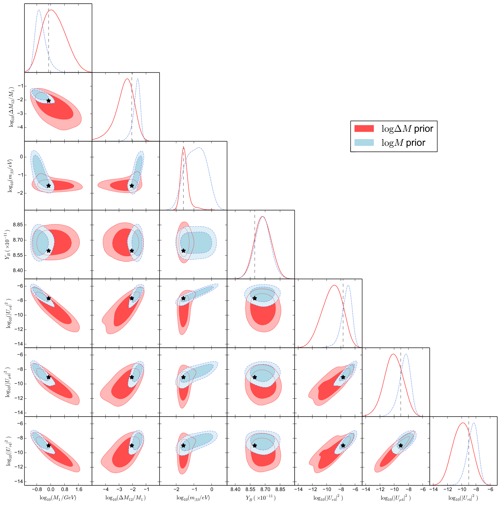
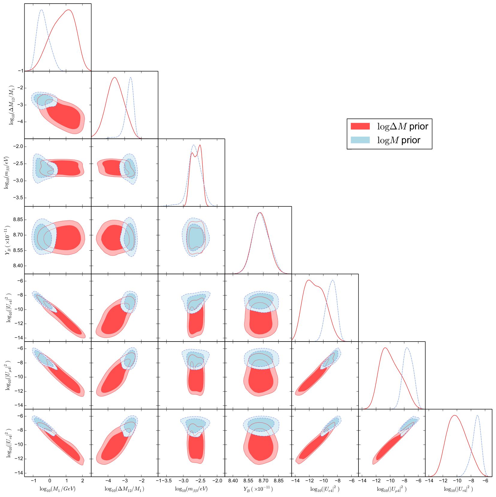
Figures 4 and 5 show, for IH and NH, the posterior probabilities of the spectrum of the two relevant states, , the active-sterile mixings of the first heavy state (those of the second state are almost identical), the neutrinoless double beta decay effective mass and the baryon asymmetry . An important consideration are the priors. We have considered flat priors in all the Casas-Ibarra parameters except the masses where we assume a flat prior in , within the range , and two possibilities: 1) a flat prior also in in the same range or 2) a flat prior in in the range . The two different colours (light blue and red) in Fig. 4 correspond to the two options. The significant differences between the two posteriors show the effect of allowing or not for fine-tuning in the degeneracy of the two heavy states. Even though the contours are typically larger if more fine-tuning is allowed, we find interesting solutions with a mild degeneracy, which tend to imply smaller , larger values of the active-sterile mixing parameters and a sizeable non-standard contribution to neutrinoless double beta decay, which obviously imply much better chances of testability. Figs. 6 zoom in the most interesting results from this study: the mild level of fine-tuning of the blue contours (neither a strong degeneracy is required, nor a very large deviation from the naive seesaw scaling of the mixings), correlated with a relatively large mixing, and a sizeable amplitude for neutrinoless double beta decay. We will come back to this point in the next section.
In table 2 we show the 68 probability ranges for the relevant parameters as extracted from the 1D posterior probabilities, for the two neutrino orderings and the two prior choices. The ranges for the mixings of the second heavy state, , are basically the same.
| NO | Prior | ||||||
|---|---|---|---|---|---|---|---|
| IH | M | ||||||
| M | |||||||
| NH | M | ||||||
| M |
In Figures 7 we zoom in the probability plots for the heavy neutrino mixings versus mass and compare them with present [33],[34] and future constraints from DUNE [35], SHiP [36] and FCC [37]. Constraints from Big Bang Nucleosynthesis are very restrictive in the low mass range, particularly below the pion threshold [38, 39].
In ref. [15] similar figures were shown from a scan of parameter space assuming only flat priors in and . We note that the regions we show here are the result of a full numerical treatment, that avoids any constraint in parameter space and successfully explain the baryon asymmetry within its small uncertainty. The most important addition is however that of the blue contours that use flat priors in and , and therefore avoid too large fine-tuning. These solutions point to a region of parameter space within SHiP reach as the most probable one. It is interesting that the sensitivity of SHiP and DUNE to the or channels will cover to a large extent the blue regions. When a larger degree of degeneracy in the masses is allowed (red regions), the right baryon asymmetry can be obtained also for larger masses, up to 10-100 GeV, but this high mass region will be harder to test experimentally (for recent work see also [40]).
In the case, there are 13 unknown parameters and the exploration of parameter space is significantly more challenging. This case will be considered elsewhere.
4 Predicting the baryon asymmetry in the minimal model
A very relevant question is whether the baryon asymmetry could be predicted in this scenario if the heavy sterile neutrinos are within reach of future experiments, such as the SHiP experiment. We will analyse this question in the simplest case where the number of unknown parameters is minimal. Obviously the situation for the case will be much more difficult.
The SHiP experiment will be capable of detecting heavy neutrinos in the few GeV range provided their mixings are sufficiently large. In particular significantly larger than what the naive seesaw scaling would suggest. In the Casas-Ibarra parametrization of eq. (14), this implies that the entries of the matrix need to be significantly larger than one, and therefore the imaginary part of the complex angle needs to be sizeable.
In order to understand the dependence of on the different parameters, it is useful to consider the perturbative results of [15]. The CP asymmetries responsible for the baryon number generation, , in the weak washout regime, can be generically written as
| (57) |
with
| (58) |
For the case, when and , this quantity can be written as [15]
| (59) |
where the invariants are defined in eq. (44). This is indeed the dependence obtained from the solution of the kinetic equations in the perturbative approximation obtained in [15], in the weak washout limit. For our new kinetic equations, the perturbative result is shown in eq. (46) (where only the contribution has been kept). We can read from eq. (46) in the limit of weak washout, , and using eq. (54):
| (60) |
In contrast with eq. (46), this approximation fails at large times since it is valid only for . It typically overestimates the asymmetry, but should give qualitatively the right dependence on the parameters.
What we need however are the expressions in terms of the Casas-Ibarra parameters. The relations are typically very complicated, but we can identify a few small parameters and perturb in them:
| (61) |
where , assumed positive, is the imaginary part of the complex angle of the matrix that needs to be large to avoid the naive seesaw scaling of the active-sterile mixings 33 3 Note that can also be negative, but there is an approximate symmetry , that would lead to very similar results by expanding in in this case. . Defining
| (62) |
the result for the heavy-light mixing for IH can be written as
The result for NH is:
Note that the mixings depend exponentially on and are inversely proportional to the heavy masses, but this dependence drops in any ratio.
At leading order (LO) in the expansion, we see that for IH, the ratio of the electron and muon mixings is independent of and heavy masses and depends exclusively on the Majorana CP phase of the PMNS matrix, :
| (65) |
This is important because the CP asymmetry strongly depends on this phase as we will see below, therefore for the IH, the putative measurement of the masses and the mixings of these states in SHiP for example, would allow in principle to fix simultaneously and . For NH on the other hand the SHiP measurement would only provide information on but not on nor any other phase, at this order:
| (66) |
The mixings to taus are at this order the same as those to muons.
The leading order however is not precise enough. For IH, it is clear from eq. (65) that depending on the value of a significant suppression of the leading terms in the numerator or denominator can take place, therefore at this point the NLO corrections are relevant and these bring a new undetermined parameter, , as can be seen from eqs. (), which is the CP phase that can be measured in neutrino oscillations! In this case, the measurement of the ratio of mixings at SHiP cannot resolve and simultaneously and a degeneracy between these two phases remains. We will come back to this interesting observation in the following section. Clearly the phase could be determined in future neutrino oscillation experiments.
At leading order in the expansion, the CP asymmetry in this regime can be approximated by
where in the case of NH we have included NLO corrections because the LO cancel for maximal atmospheric mixing. We see that for both neutrino orderings, it depends strongly on the real part of the Casas-Ibarra angle , which does not affect any other of the observables above. In particular, independently of the value of , there is always a value of that can make the asymmetry vanish. For instance for the IH result the value can be approximated by
| (68) |
therefore the uncertainty in forbids to set a lower bound on the asymmetry, although an upper bound can be derived. Therefore even if the sterile states would be discovered at SHiP and their mixings to electrons and muons accurately measured, the asymmetry can only be predicted up to this angle.
Furthermore as we have seen in order to explain the baryon asymmetry in the case, a significant level of degeneracy between the two states is needed. The dependence on this quantity enters in the function . Although we have not found a detailed study of the expected uncertainty in the invariant mass at SHiP, given the momentum resolution for muons and pions quoted in [41], we expect that this uncertainty could be better than 1. If the degeneracy cannot be measured, a large uncertainty in the CP asymmetry will result also from this unknown.
Interestingly neutrinoless double beta decay also depends on both unknowns: and . The effective neutrino mass in neutrinoless double beta is given approximately by [42, 43]
| (69) | |||||
| (70) | |||||
where the two lines in each amplitude correspond respectively to the light and heavy contributions. depends on the nucleus under consideration. For 48Ca, 76Ge, 82Se, 130Te and 136Xe, 0.035, 0.028, 0.028, 0.033 and 0.032, respectively [44, 45]. Since is very small we have neglected effects in the heavy contribution.
Note that the non-standard contribution from the heavy states is very sensitive to the mass degeneracy. Furthermore the interference between the light and heavy contributions is very sensitive to the angle , and it is precisely in the region around 1 GeV where the heavy and light contributions can be comparable, and can effectively interfere [46, 47, 43]. There is therefore the possibility that neutrinoless double beta decay could provide the missing information to predict the baryon asymmetry.
On the left plot of Fig. 8 we show as a function of the angle for IH and some choice of parameters that are within the range of SHiP and assumed known. has been computed exactly using the nuclear matrix elements for 76Ge from ref. [44].The bands are the standard contributions to for NH/IH. If the uncertainty in could be better than the spread within the standard IH region, a determination of could result from this measurement. On the right plot we show the dependence of (computed exactly) on the same angle. In Fig. 9 we show the correlation between and as we vary .
Ideally a precise determination of could predict the baryon asymmetry up to a global sign. In practice, this would require a very good control of the nuclear matrix elements which is very challenging.
As a proof of principle we have studied the posterior probabilities for a hypothetical measurement of SHiP of and and their respective couplings to electrons and muons for IH. The point chosen is indicated by a star in Fig. 4. We did not look for a very special nor optimal point, simply that it was within the range of SHiP and could explain the baryon asymmetry. The corresponding triangle plots are shown in Fig. 10 for two values of the assumed errors in this experiment: relative errors on masses and mixings of and the much more optimistic .
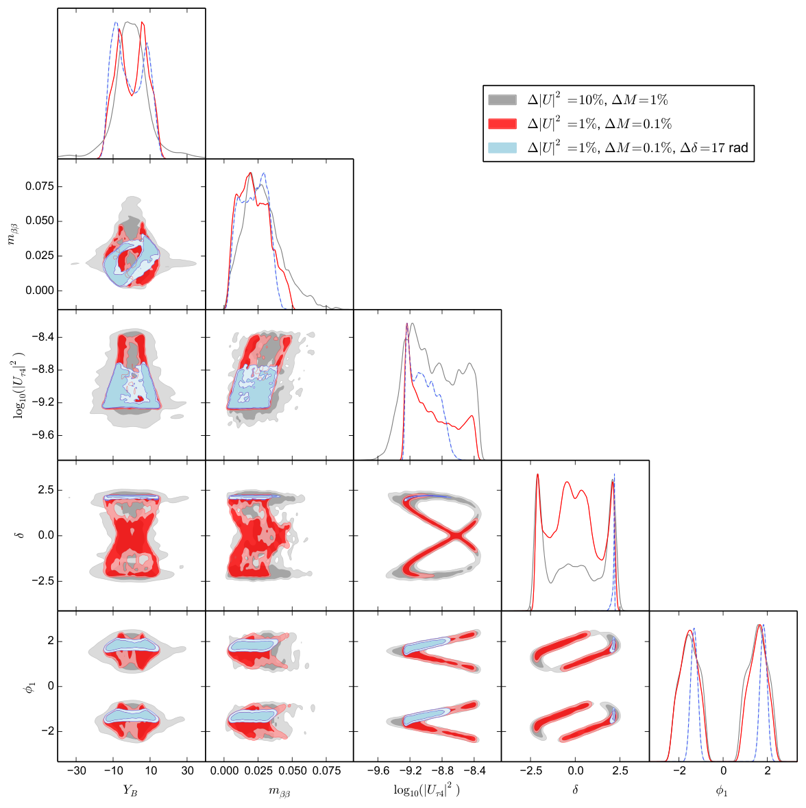
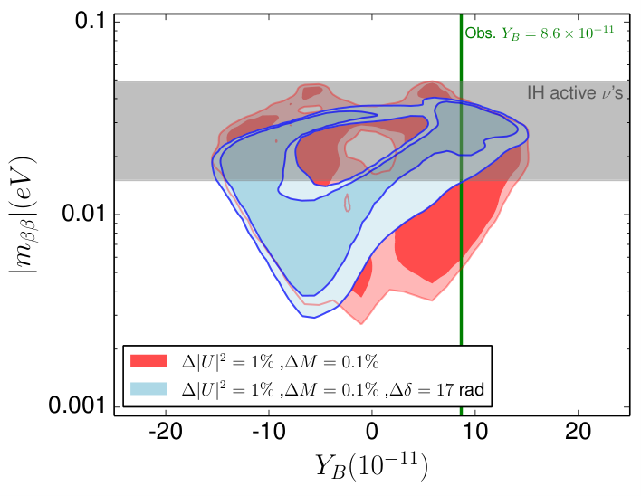
We furthermore considered a combination of SHiP, with the more optimistic errors, with a determination of in future neutrino oscillation experiments such as HyperK and DUNE. We have assumed as derived from the studies in references [48, 49]. The versus plot is zoomed in in Fig. 11.
Clearly the determination of results in a more clear correlation between and . In fact the resulting width of the contour can be understood from the propagation of the error in on the determination of . This is shown in Fig. 12, where we compare the posterior probability with the three curves obtained in the following way: 1) fixing the parameters to those of the test point and changing only (solid line), 2) the same as 1) except which is fixed to , and correspondingly tuned to keep the mixings unchanged. There are two solutions for and the two dashed lines correspond to the two values (see Fig. 13), according to the analytical approximate formulae. The region encompassed by these lines is roughly similar to the and regions.
For NH, the expectations are much more pessimistic, since the SHiP measurement would have a hard time to pin down , even if is known, and therefore two unknowns would remain. They could be determined in principle from a measurement of and but not from one single measurement and therefore the baryon asymmetry will be very difficult to predict in this case. The measurement of for NH would nevertheless be futuristic since the value would be roughly a factor 10 smaller, which is beyond the reach of the next generation of neutrinoless double beta decay experiments.
5 phases from SHiP and neutrinoless double beta decay
We have seen that the ratios of electron and muon mixings that could be measured at SHiP could give very interesting information of the phases of the PMNS matrix. We stress that this is independent of whether the baryon asymmetry can be explained or not. This relies on the fact that the mixings are large enough so that they can be discovered at SHiP. In this case, the ratio of the electron to muon mixings are dominantly controlled by the phases of the PMNS mixing matrix, as can be seen in eqs. () and ().
In Fig. 13, we compare the correlation expected on the plane from a putative measurement of this ratio using the analytical formulae of eqs. () for the test point of the previous section, to the posterior probabilities obtained with the most competitive SHiP uncertainties assumed in the previous section. Clearly the analytical formulae work very well and demonstrate the potential of SHiP in constraining the CP violating phases of the mixing matrix.
This has the following interesting consequence. If neutrinoless double beta decay could be measured with sufficient precision and the effect of the unknown would be small (this would happen for example in a more degenerate situation or for larger heavy masses which suppress the heavy contribution to neutrinoless double beta decay), the combination of this measurement with that at SHiP could provide information on the phase . Quantifying what is the reach of the combination of SHiP and neutrinoless double beta decay on is very interesting and deserves a dedicated study.
Reversely, if a measurement of could be obtained from neutrino oscillation measurements, a putative measurement of SHiP could provide a more precise prediction of the neutrinoless double beta decay amplitude if the neutrino ordering is inverted. This would be an extra motivation for improving the nuclear matrix element determination.
The possibility of measuring also the tau mixing at SHiP could help to resolve the degeneracy. Fig. 14 shows the isocurves of and in the plane. The test point we used did not have sensitivity to the tau mixing according to the expectations for SHiP, but if this measurement could be improved this would also be useful to reduce the degeneracy.
6 Conclusions
We have studied the production of the matter-antimatter asymmetry in low-scale seesaw models. We have improved our previous study [15] by including the washout processes from gauge interactions and Higgs decays and inverse decays, quantum statistics in the computation of all rates, as well as spectator processes. This together with a more efficient numerical treatment of the equations have allowed us to perform the first bayesian exploration of the full parameter space that explains the observed baryon asymmetry in the context of the minimal model, where only two singlets play a role in the generation of the baryon asymmetry.
We have demonstrated that successful baryogenesis is possible with a mild heavy neutrino degeneracy, and more interestingly that these less fine-tuned solutions prefer smaller masses GeV, which is the target region of SHiP, and significant non-standard contributions to neutrinoless double beta decay. We have also demonstrated the complementarity of future putative measurements from SHiP, neutrinoless double beta decay and searches for leptonic CP violation in neutrino oscillations, in the quantitative prediction of the baryon asymmetry within the minimal model. If singlets with masses in the GeV range would be discovered in SHiP and the neutrino ordering is inverted, the possibility to predict the baryon asymmetry (maybe up to a sign) looks in principle viable, in contrast with previous beliefs. Unrelated to whether the baryon asymmetry is explained or not, we have also shown that a measurement of the electron and muon mixings of heavy species within SHiP range could precisely determine, in the minimal model, a combination of the two phases of the matrix.
Acknowledgements.
We warmly thank N. Rius for useful discussions and earlier collaboration. This work was partially supported by grants FPA2014-57816-P, PROMETEOII/2014/050, and the European projects H2020-MSCA-ITN-2015//674896-ELUSIVES and H2020-MSCA-RISE-2015. PH acknowledges the support of the Munich Institute for Astro- and Particle Physics (MIAPP) of the DFG cluster of excellence Origin and Structure of the Universe to participate in the workshop Why is there more matter than antimatter in the Universe, where this work was first presented prior to publication [50].References
- (1) M. Fukugita and T. Yanagida, Baryogenesis Without Grand Unification, Phys.Lett. B174 (1986) 45.
- (2) S. Davidson and A. Ibarra, A Lower bound on the right-handed neutrino mass from leptogenesis, Phys. Lett. B535 (2002) 25–32, [hep-ph/0202239].
- (3) T. Hambye, Y. Lin, A. Notari, M. Papucci and A. Strumia, Constraints on neutrino masses from leptogenesis models, Nucl. Phys. B695 (2004) 169–191, [hep-ph/0312203].
- (4) J. Racker, M. Pena and N. Rius, Leptogenesis with small violation of B-L, JCAP 1207 (2012) 030, [1205.1948].
- (5) A. Pilaftsis and T. E. J. Underwood, Resonant leptogenesis, Nucl. Phys. B692 (2004) 303–345, [hep-ph/0309342].
- (6) S. Davidson, E. Nardi and Y. Nir, Leptogenesis, Phys.Rept. 466 (2008) 105–177, [0802.2962].
- (7) E. K. Akhmedov, V. Rubakov and A. Y. Smirnov, Baryogenesis via neutrino oscillations, Phys.Rev.Lett. 81 (1998) 1359–1362, [hep-ph/9803255].
- (8) T. Asaka and M. Shaposhnikov, The nuMSM, dark matter and baryon asymmetry of the universe, Phys.Lett. B620 (2005) 17–26, [hep-ph/0505013].
- (9) M. Shaposhnikov, The nuMSM, leptonic asymmetries, and properties of singlet fermions, JHEP 0808 (2008) 008, [0804.4542].
- (10) T. Asaka, S. Eijima and H. Ishida, Kinetic Equations for Baryogenesis via Sterile Neutrino Oscillation, JCAP 1202 (2012) 021, [1112.5565].
- (11) L. Canetti, M. Drewes, T. Frossard and M. Shaposhnikov, Dark Matter, Baryogenesis and Neutrino Oscillations from Right Handed Neutrinos, Phys.Rev. D87 (2013) 093006, [1208.4607].
- (12) M. Drewes and B. Garbrecht, Leptogenesis from a GeV Seesaw without Mass Degeneracy, JHEP 03 (2013) 096, [1206.5537].
- (13) B. Shuve and I. Yavin, Baryogenesis through Neutrino Oscillations: A Unified Perspective, Phys.Rev. D89 (2014) 075014, [1401.2459].
- (14) A. Abada, G. Arcadi, V. Domcke and M. Lucente, Lepton number violation as a key to low-scale leptogenesis, JCAP 1511 (2015) 041, [1507.06215].
- (15) P. Hernández, M. Kekic, J. López-Pavón, J. Racker and N. Rius, Leptogenesis in GeV scale seesaw models, JHEP 10 (2015) 067, [1508.03676].
- (16) A. Anisimov, D. Besak and D. Bodeker, Thermal production of relativistic Majorana neutrinos: Strong enhancement by multiple soft scattering, JCAP 1103 (2011) 042, [1012.3784].
- (17) D. Besak and D. Bodeker, Thermal production of ultrarelativistic right-handed neutrinos: Complete leading-order results, JCAP 1203 (2012) 029, [1202.1288].
- (18) I. Ghisoiu and M. Laine, Right-handed neutrino production rate at T ¿ 160 GeV, JCAP 1412 (2014) 032, [1411.1765].
- (19) J. A. Casas and A. Ibarra, Oscillating neutrinos and muon —¿ e, gamma, Nucl. Phys. B618 (2001) 171–204, [hep-ph/0103065].
- (20) G. Sigl and G. Raffelt, General kinetic description of relativistic mixed neutrinos, Nucl.Phys. B406 (1993) 423–451.
- (21) E. Nardi, Y. Nir, E. Roulet and J. Racker, The Importance of flavor in leptogenesis, JHEP 01 (2006) 164, [hep-ph/0601084].
- (22) Planck collaboration, P. A. R. Ade et al., Planck 2015 results. XIII. Cosmological parameters, 1502.01589.
- (23) J. A. Harvey and M. S. Turner, Cosmological baryon and lepton number in the presence of electroweak fermion number violation, Phys. Rev. D42 (1990) 3344–3349.
- (24) M. Laine and M. E. Shaposhnikov, A Remark on sphaleron erasure of baryon asymmetry, Phys. Rev. D61 (2000) 117302, [hep-ph/9911473].
- (25) C. A. Arguelles Delgado, J. Salvado and C. N. Weaver, A Simple Quantum Integro-Differential Solver (SQuIDS), Comput. Phys. Commun. 196 (2015) 569–591, [1412.3832].
- (26) https://github.com/jsalvado/SQuIDS.
- (27) F. Feroz and M. Hobson, Multimodal nested sampling: an efficient and robust alternative to MCMC methods for astronomical data analysis, Mon.Not.Roy.Astron.Soc. 384 (2008) 449, [0704.3704].
- (28) F. Feroz, M. Hobson and M. Bridges, MultiNest: an efficient and robust Bayesian inference tool for cosmology and particle physics, Mon.Not.Roy.Astron.Soc. 398 (2009) 1601–1614, [0809.3437].
- (29) F. Feroz, M. P. Hobson, E. Cameron and A. N. Pettitt, Importance Nested Sampling and the MultiNest Algorithm, 1306.2144.
- (30) https://github.com/cmbant/getdist.
- (31) M. C. Gonzalez-Garcia, M. Maltoni and T. Schwetz, Updated fit to three neutrino mixing: status of leptonic CP violation, JHEP 11 (2014) 052, [1409.5439].
- (32) L. Canetti and M. Shaposhnikov, Baryon Asymmetry of the Universe in the NuMSM, JCAP 1009 (2010) 001, [1006.0133].
- (33) A. Atre, T. Han, S. Pascoli and B. Zhang, The Search for Heavy Majorana Neutrinos, JHEP 05 (2009) 030, [0901.3589].
- (34) F. F. Deppisch, P. S. Bhupal Dev and A. Pilaftsis, Neutrinos and Collider Physics, New J. Phys. 17 (2015) 075019, [1502.06541].
- (35) LBNE collaboration, C. Adams et al., The Long-Baseline Neutrino Experiment: Exploring Fundamental Symmetries of the Universe, 2013. 1307.7335.
- (36) S. Alekhin et al., A facility to Search for Hidden Particles at the CERN SPS: the SHiP physics case, 1504.04855.
- (37) FCC-ee study Team collaboration, A. Blondel, E. Graverini, N. Serra and M. Shaposhnikov, Search for Heavy Right Handed Neutrinos at the FCC-ee, in Proceedings, 37th International Conference on High Energy Physics (ICHEP 2014), 2016. 1411.5230. DOI.
- (38) A. D. Dolgov, S. H. Hansen, G. Raffelt and D. V. Semikoz, Heavy sterile neutrinos: Bounds from big bang nucleosynthesis and SN1987A, Nucl. Phys. B590 (2000) 562–574, [hep-ph/0008138].
- (39) O. Ruchayskiy and A. Ivashko, Restrictions on the lifetime of sterile neutrinos from primordial nucleosynthesis, JCAP 1210 (2012) 014, [1202.2841].
- (40) S. Antusch, E. Cazzato and O. Fischer, Displaced vertex searches for sterile neutrinos at future lepton colliders, 1604.02420.
- (41) SHiP collaboration, M. Anelli et al., A facility to Search for Hidden Particles (SHiP) at the CERN SPS, 1504.04956.
- (42) A. Ibarra, E. Molinaro and S. T. Petcov, Low Energy Signatures of the TeV Scale See-Saw Mechanism, Phys. Rev. D84 (2011) 013005, [1103.6217].
- (43) J. Lopez-Pavon, E. Molinaro and S. T. Petcov, Radiative Corrections to Light Neutrino Masses in Low Scale Type I Seesaw Scenarios and Neutrinoless Double Beta Decay, JHEP 11 (2015) 030, [1506.05296].
- (44) M. Blennow, E. Fernandez-Martinez, J. Lopez-Pavon and J. Menendez, Neutrinoless double beta decay in seesaw models, JHEP 07 (2010) 096, [1005.3240].
- (45) A. Ibarra, E. Molinaro and S. T. Petcov, TeV Scale See-Saw Mechanisms of Neutrino Mass Generation, the Majorana Nature of the Heavy Singlet Neutrinos and -Decay, JHEP 09 (2010) 108, [1007.2378].
- (46) M. Mitra, G. Senjanovic and F. Vissani, Neutrinoless Double Beta Decay and Heavy Sterile Neutrinos, Nucl. Phys. B856 (2012) 26–73, [1108.0004].
- (47) J. Lopez-Pavon, S. Pascoli and C.-f. Wong, Can heavy neutrinos dominate neutrinoless double beta decay?, Phys. Rev. D87 (2013) 093007, [1209.5342].
- (48) DUNE collaboration, R. Acciarri et al., Long-Baseline Neutrino Facility (LBNF) and Deep Underground Neutrino Experiment (DUNE), 1512.06148.
- (49) Hyper-Kamiokande Proto-Collaboration collaboration, K. Abe et al., Physics potential of a long-baseline neutrino oscillation experiment using a J-PARC neutrino beam and Hyper-Kamiokande, PTEP 2015 (2015) 053C02, [1502.05199].
- (50) https://users.ph.tum.de/ga24wax/2016_W3_slides/Hernandez_slides.pdf.