A dynamical adaptive tensor method for the Vlasov-Poisson system
Abstract
A numerical method is proposed to solve the full-Eulerian time-dependent Vlasov-Poisson system in high dimension. The algorithm relies on the construction of a tensor decomposition of the solution whose rank is adapted at each time step. This decomposition is obtained through the use of an efficient modified Progressive Generalized Decomposition (PGD) method, whose convergence is proved. We suggest in addition a symplectic time-discretization splitting scheme that preserves the Hamiltonian properties of the system. This scheme is naturally obtained by considering the tensor structure of the approximation. The efficiency of our approach is illustrated through time-dependent 2D-2D numerical examples.
1 Introduction
The present work investigates a numerical method for the resolution of the time-dependent Vlasov-Poisson system. The solution is approximated using parsimonious tensor methods.
In the litterature, equations arising in kinetic theory are solved by three classes of approaches: particle methods (Particle-In-Cell [22, 4, 8], Particle-In-Cloud [42]), semi-lagrangian approaches [13, 9, 29, 37, 14] and full-deterministic Eulerian methods [21, 33, 43]. In this work, we focus on the Vlasov-Poisson system as a simple yet challenging example of kinetic equation. While Eulerian approaches are appealing to describe the evolution of the unknown quantities of interest, the high dimensionality of the phase space domain make them often prohibitive in terms of memory and computational cost, especially when 2D-2D and 3D-3D problems are at hand.
The proposed method is not a particular discretization per se, instead, it gives a way to build a parsimonius tensor decomposition starting from chosen a priori separated discretizations for the space and the velocity variables in a full eulerian approach. The contribution is twofold: first, we show that the use of a tensorised representation of the solution induces a natural splitting of the equations which respects the Hamiltonian nature of the Vlasov-Poisson equations; second, an efficient fixed-point algorithm is proposed to solve the (non-symmetric) equations using tensorised functions. This step is performed using a modified Proper Generalized Decomposition (PGD) method [11, 20, 10, 19, 18, 5, 31], and the convergence of the scheme is proved. Let us mention that close ideas were introduced in the recent work [12] for the evolution of high-dimensional probability densities. In the contribution [29], a tensor train method is used to discretize the Vlasov-Poisson equations by separating each component, in a semi-lagrangian approach.
Here, we do not separate in all the variables in order to deal with generic space (and possibly velocity) domain geometries [43]. Thus, only second order tensors are used. The proposed method dynamically adapts through time the rank of the decomposition. This is an important feature, as was noted in [12, 29], since the number of tensorised terms needed to approximate with a given tolerance the solution at a certain time is not known a priori.
The structure of the work is as follows: in Section 2, the Vlasov-Poisson system is recalled in its classical and Hamiltonian formulation. A discussion on how a tensorised representation leads to a natural splitting of the evolution is presented in Section 2.3.
A second-order symplectic scheme in time is derived for the tensor representation update. Then, in Section 3, after a brief review of the PGD method for the resolution of symmetric coercive problems, a fixed-point scheme is presented, to solve some non-symmetric linear problems arising in the Vlasov-Poisson context. The proof of convergence of the algorithm is presented in Appendix A. Numerical tests illustrating the properties of the method are presented in Section 5.
2 Hamiltonian formulation and tensor decomposition
In this section, the Hamiltonian formulation of the Vlasov-Poisson system is recalled. A particular emphasis is put on the elements that play an important role in the derivation of the proposed numerical method. The idea is to compute a tensor decomposition of the solution of the Vlasov-Poisson system and to use a symplectic integrator in time in order to preserve the hamiltonian structure of the equations. As it will be shown in Section 2.3, the tensorised expansion induces a natural splitting of the equations.
2.1 The Vlasov-Poisson system
Let denote the spatial dimension of the problem and . The Vlasov-Poisson system for negative electric charges reads:
| (1) |
with appropriate boundary conditions on , where
is the particle distribution function in the phase space, is the initial particle distribution function, the electric fied and the electric potential. The particle density is given by , and hence, the equation for the electric potential reads .
The global existence of positive (weak or strong) solutions has been studied in several works [2, 3, 16, 32, 23, 28, 1].
For instance, in [32], when , the existence of a strong non-negative solution is proved provided that the initial condition satisfies the additional condition: for some ,
2.2 Hamiltonian formulation
The Hamiltonian for the Vlasov-Poisson system reads:
| (2) |
The first term in the Hamiltonian is the kinetic energy of the particles, and the second term accounts for the electro-static energy. As commented in [34], the Vlasov-Poisson equations can be derived by introducing a reduced Poisson bracket:
| (3) |
2.3 Splitting induced by tensor decomposition
For any measurable functions and , we define the tensor product function as
In the sequel, such a function is referred to as a pure tensor-product function. A linear combination of pure tensor-product functions (for some ) is called a rank- tensor product function.
We also introduce here the notion of tensorized operators. Let (respectively ) be a Hilbert space of real-valued functions defined on (respectively on ) and a Hilbert space of functions defined on so that . An operator acting on functions depending on both and variables is a tensorized operator if it can be written as
for some , where for all , (respectively ) is an operator on (respectively on ). Let us remind the reader that for all operators on , on , and ,
In this section, a formal calculation is presented, which justifies how such a decomposition induces a natural splitting of the Vlasov-Poisson equations. Let us mention here the work [7], where a high-order splitting of the hamiltonian formulation for the Vlasov-Maxwell system was recently proposed.
In the present method, the aim is to approximate the function , solution of (1), by a separate variate expansion of the form:
| (5) |
with some measurable functions , and . When this expression is inserted into the evolution equation written in a hamiltonian form, it reads:
| (6) |
The Poisson bracket acting on and , separately, can be interpreted as the operator which is inducing a dynamics on the functions and . Indeed, when considering and , the tensor decomposition implies naturally . Consider a particular time , for which . The action of the Poisson bracket on generic functions and depending respectively only upon the space coordinate or the velocity reads:
| (7) | |||
| (8) |
Two facts are fundamental: first, the evolution operator splits naturally into two parts, one acting on and the other on . Second, the evolution of each part is the action of a tensorised operator acting on the functions.
2.4 Symplectic integrator in time
Let us define and as solutions to the dynamical system:
| (9) |
At , it holds that
| (10) |
In other words, the time derivative of a generic element computed at time is given by the advection part of the Vlasov-Poisson system, whereas the time derivative of the element is given by the electrostatic force. Remark that initial functions at time depend only upon , but the time derivative depends of course also on . The analogue is true for the functions.
A symplectic discretization in time for the system (4) is proposed, based on this remark. For a comprehensive overview of geometric integrators see [27]. Let be a small time step. The starting point is to consider the system (10) and use a Störmer-Verlet algorithm (see [26]) to discretize the evolution of the functions and between times and . This scheme is obtained by considering and as if they were the coordinates and the momenta of the Hamiltonian system associated to the Vlasov-Poisson equation. Define , , and , and as follows:
| (11) | |||
| (12) | |||
| (13) |
where the definitions of the electric fields are given below. Remember that . We define and by
| (14) | |||
and
| (15) | |||
Defining
the above scheme can be rewritten as
| (17) | |||
This naturally leads us to define the following time-discretization scheme for the evolution of . Set and for all , define
| (18) | |||
The function then gives an approximation of the solution to (1) at time .
Of course, the starting point of the derivation of this scheme was to postulate that the function can be written in a separate variate expansion at some time . In the next section, we present the algorithm which is used at each substep of the time-discretization scheme in order to obtain a tensorized approximation of the functions , and for all , assuming that is given in a tensorized form.
3 Tensor methods
In this section, let , and be some arbitrary Hilbert spaces so that . A tensor-based method is introduced to solve the following problem: find solution of
| (19) |
where
- —
is a finite-rank tensor product element of ;
- —
is a small constant;
- —
is an operator on of the form where (respectively ) is a symmetric continous coercive operator on (respectively );
- —
is an arbitrary tensorized operator on (not necessarily symmetric).
In the Vlasov-Poisson context, each step of the proposed time-discretization scheme (18) can be written under the form (19). Remark that the methodology presented hereafter can be directly applied to other time-discretization schemes and other contexts provided that they only require the resolution of elementary subproblems of the form (19).
The approach relies on the so-called Proper Generalised Decomposition (PGD) method [30, 10, 11, 18, 36], and we first review well-known results about this method in Section 3.1. We stress on the properties of this method on an important particular case in Section 3.2. The scheme we propose is presented in Section 3.3 along with convergence results whose proofs are postponed to the appendix.
Let us highlight the philosophy of the method: the solution of (19) is approximated as a sum of tensor products
where for all , and . Each pair appearing in the above sum is computed in an iterative way so that the tensor product is the best possible tensor product at iteration of the algorithm. The meaning of this sentence will be made clear in the rest of the section. In the Vlasov-Poisson context, the advantage of this approach is that it only requires the resolution of linear problems for functions depending only on or only on . Thus, the sizes of the linear problems that are solved are much smaller than the one of the full linear problems defining the iterations of the scheme (18). We comment further on this point in Section 3.4.
3.1 PGD for coercive symmetric problems
The PGD method is related to the so-called greedy algorithms [39, 31] in nonlinear approximation theory. We review here well-known results on PGD algorithms for the approximation of high-dimensional coercive symmetric problems. We refer the reader to [19, 5, 20] for more details.
Let a symmetric coercive continuous bilinear form on and a continuous linear form on . Let the unique solution of the linear problem
| (20) |
The existence and uniqueness of a solution to problem (20) is a consequence of the Lax-Milgram lemma. Besides, is equivalently the unique solution of the minimization problem
were
Let us assume that the two Hilbert spaces and satisfy the following assumptions:
- (H1)
and the inclusion is dense in ;
- (H2)
is weakly closed in .
Before presenting the PGD algorithm, we give here two simple examples of Hilbert spaces that satisfy these assumptions and are interesting in the Vlasov-Poisson context.
- 1.
When , the spaces and satisfy assumptions (H1)-(H2) [5].
- 2.
In a discretized setting, when for some , the choice and ensures that (H1)-(H2) holds.
Let be a given vector (which is usually chosen as . The PGD algorithm to compute an approximation of starting from the initial guess reads as follows:
PGD algorithm: — Initialization: Set and . — Iterate on : Compute as a solution of the minimization problem (21) where for all , . Define and set .
The choice of a stopping criterion is an important issue and we comment it later in this article. The method used in practice to solve (21) is detailed in Section 3.4.
The following convergence result holds:
Proposition 1.
Assume that the spaces satisfy assumptions (H1)-(H2). Then, all the iterations of the PGD algorithm are well-defined in the sense that there exists at least one solution to problem (21) for all . Besides, the sequence strongly converges in to .
We refer the reader to [31, 5, 19, 20] for more details on the method and for the proof of this result. No further assumption is required at this stage on a or b for the convergence to hold. We will see in Section 3.4 that the efficiency of a PGD-based method in practice depends on the tensor decomposition of a and b.
3.2 An important particular case
A remarkable situation occurs when and . In this case, it holds that
| (22) |
Let be a small positive constant which characterizes the stopping criterion.
PGD- algorithm: — Initialization: Set and . — Iterate on : Compute as a solution of the minimization problem (23) where forall , . Define . If , then stop and define . Otherwise, set and iterate again.
Denoting by the Riesz representative of the linear form b for the scalar product , it holds that for all , is equivalently the solution of
| (24) |
Using the norm-product property (22), it can be proved [31] that if , the above algorithm gives an iterative method to compute the Proper Orthogonal Decomposition (POD) of the Riesz representative of the linear form b for the scalar product . A consequence is that an approximate solution computed after iterations of the PGD algorithm is a best -rank approximation of . In other words,
This optimality property is particularly interesting in the present case. In the rest of the article, we shall denote by .
Another interesting consequence is that the sequence of the norms of the tensor product functions given by the PGD algorithm is non-increasing. Indeed, this sequence is identical to the set of the singular values of the POD of in in non-increasing order [31].
Let us comment here on the use of this particular stopping criterion, which is the one we use in practice in the Vlasov-Poisson context. It holds from (23) (or equivalently (24)) that
For any element , let us define
The application defines a norm on which is called the injective norm [24]. This norm is equal to the maximal singular value of the POD decomposition of in . Of course, we have but these two norms are not equivalent. Thus, can be seen as the injective norm of the residual of the decomposition . We use the injective norm in practice as a stopping criterion because the latter quantity is much faster to evaluate than the -norm.
3.3 Fixed-point PGD algorithm for weakly non-symmetric problems
Assume now that is the solution of a problem of the form
| (25) |
where b is a continuous linear form on and is a continuous bilinear form which is not symmetric nor coercive in general. There exists a unique solution of this problem for instance when .
We still assume that we start from an initial guess for given by an element . A natural idea to solve (25) when is a small perturbation of the identity operator on is to consider the following fixed-point PGD algorithm:
Fixed-point PGD algorithm: — Initialization: Set and . — Iterate on : Compute as a solution of the minimization problem (26) where for all , . Define and set .
This algorithm was already suggested and studied in [6]. Its convergence was then proved under the condition that the Hilbert spaces and are finite-dimensional and that where was some constant depending on the dimension of the spaces which goes to as the dimension of the spaces go to infinity. This theoretical convergence result was much more pessimistic than the numerical observations. Indeed, it was already pointed out in [6] that numerical tests indicated that this constant should not depend on the dimension of the spaces.
In this article, we prove that does not need to depend on the dimension of the Hilbert spaces, but on the number of terms appearing in the tensor decomposition of . More precisely, let be the continuous linear operator on associated to , i.e. such that
Then, the following result holds:
Proposition 2.
All the iterations of the Fixed-point PGD algorithm are well-defined, in the sense that for all , there exists at least one solution to (21). Moreover, let us assume that where for all , and . Let . Assume that at least one of these two assumptions is satisfied:
- (A1)
(thus the norm of satisfies the norm-product property (22)) and ;
- (A2)
.
Then, there is a unique solution to (25) and the sequence strongly converges in to .
The proof of Proposition 2 is given in the appendix. Let us point out that the convergence of the proposed algorithm is not covered in the work [25], where the authors also treat approximation of equations using tensor methods and fixed-point iterations, but with a different point of view.
In the Vlasov-Poisson context, a similar stopping criterion is used, as the one we described in Section 3.2. More precisely, for , , we consider the following algorithm:
Fixed-point PGD- algorithm: — Initialization: Set and . — Iterate on : Compute as a solution of the minimization problem (27) where for all , . Define . If , then stop and define . Otherwise, set and iterate again.
Let denote the Riesz representative of b in . For all , is a solution to (26) if and only if it is a solution to
| (28) |
where denotes the identity operator on . The stopping criterion used above is justified by the fact that, for all , is equal to the injective norm of the residual of the equation . Indeed, (28) implies that
3.4 Alternating least squares (ALS) for the practical resolution of the PGD iterations
We present in this section how minimization problems (21), (23), (26) and (27) are solved in practice. Let us point out that in all cases, at iteration , is defined as a solution to
| (29) |
where for all , , for some continuous linear form and coercive bilinear continuous form , wich depend on .
Problem (29) is solved in practice using the Alternating Least Squares (ALS) [17, 40, 38] algorithm which is standard in tensor-based approximation methods. For a given error tolerance , the algorithm reads as follows:
ALS- algorithm: — Initialization: Set and choose randomly and . — Iterate on : Compute as the unique solution of (30) Then, compute as the unique solution of (31) If , set and . Otherwise, set and iterate again.
The convergence properties of this ALS algorithm are analyzed in details in [17] in the case when and are finite-dimensional, and for more sophisticated tensor formats. The algorithm can be shown to converge to a solution of the Euler equations associated to (29). The limit tensor product is not theoretically ensured to be the global minimum (or even a local minimum) of .
However, in practice, one can observe that it usually converges in a few iterations to a local minimum of (29). It is very commonly observed that this choice leads to very satisfactory convergence rates of PGD methods. Hence, we also use it here in the Vlasov-Poisson context.
In the rest of the article, we shall denote by (respectively ) the functions obtained by the PGD- (respectively Fixed-point PGD-) method when minimization problem (24) (respectively (27)) is solved using an ALS- algorithm. We also denote by .
We stress here on a crucial point: for the ALS algorithm to be numerically efficient in a high-dimensional context, it is important that the forms c and l admits a finite-rank tensor decomposition. Indeed, let us assume that and for some , such that for all , , , and for all , , .
At each iteration of the ALS- algorithm, (respectively ) is the unique solution to (30) (respectively (31)) if and only if it is the solution of the first-order Euler equations
We clearly see that the computation of and only requires the resolution of a linear symmetric coercive system for functions depending only on , or only on . The size of the associated discretized problems are thus much smaller than those that one would have obtained to solve (25) directly for instance.
Using the tensor decomposition of c and l, these equations can be rewritten as
| (32) | |||
| (33) | |||
The tensorized decomposition of c and l implies that each term appearing in (33) and (33) can be quickly evaluated, since they only involve forms defined on Hilbert spaces of functions depending on only one variable. Such tensorized decompositions are always naturally available in the Vlasov-Poisson context, and this crucial fact is at the heart of the efficiency of this approach.
4 Final algorithm for the Vlasov-Poisson system
4.1 Space and velocity discretization
Let us highlight that the proposed method can be adapted to various types of space and velocity discretizations, as well as different time schemes. It can also be adapted in other contexts than the Vlasov system. Let us assume that a discretization with (respectively ) degrees of freedom in the variable (respectively the variable) is used. Thus, at each time step of the discretization scheme, the approximation of is characterized by a matrix which is computed in a separated form as
with some vectors and .
In this setting, the Hilbert spaces , and are chosen to be , and . The only requirement for this strategy to be applicable is that each step of the chosen scheme requires the resolution of problems of the form (19), where is a tensorized operator at the discrete level, and a finite-rank element of . More precisely, we assume that at each step of the algorithm and can be respectively written as
for some matrices , and vectors , . Also, the operator appearing in equation (19) can be written as for some symmetric positive matrices and . The space is endowed with the scalar product
The idea is illustrated using a finite element discretization. Let us introduce and some finite element discretization bases of functions defined on and respectively. Assume that these functions belong respectively to and with appropriate boundary conditions.
The following matrices are defined: for all (recall that is the dimension of the problem), and any measurable bounded field ,
The time scheme introduced in Section 2.4 is recalled:
| (34) | |||
The discretized version of this scheme then reads as follows: let . For all , compute solutions of
| (35) | |||
4.2 Summary of the algorithm in the discretized setting
The method we propose for the resolution of the Vlasov-Poisson system is summarized hereafter. Let be a chosen tolerance threshold.
Verlet-PGD- algorithm: — Initialization: Set . — Iterate on : — Define and . Compute as Recompress by computing — Define . Compute as Recompress by computing — Define . Compute as
The condition we obtained in Proposition 2 on the convergence of the Fixed-point PGD algorithm implies that the time step has to be taken sufficiently small to ensure that the norms of the operators entering in the decomposition of and are also small. In practice, we thus observe that our scheme suffers from a type of CFL condition that has to be respected for the method to converge. Apart from this restriction which does not appear to be too penalizing in practice, the approach proposed here is very flexible and yields promising numerical results as shown in the next section.
5 Numerical results
In this section some numerical experiments are presented, to assess the properties of the method. First, two 1D-1D examples are considered, to validate the proposed approach. The following quantities are monitored: the error in mass, momentum and energy conservation, and the error with respect to a reference solution. The averaged in time relative errors are defined as follows:
| (36) | |||
| (37) | |||
| (38) | |||
| (39) |
where is the final time of the simulation, is the normalising mass factor, defined as the mass of the initial condition , is the momentum reference value, where is the initial kinetic energy, and is the Hamiltonian at initial time.
In the last part of this section, a 2D-2D example is shown to illustrate the applicability of the method in more high-dimensional settings. Simulations on 3D-3D testcases is work in progress.
5.1 Landau Damping.
The first test proposed is a standard linear Landau damping in a 1D-1D configuration, as proposed in [33]. The domain size is and . Periodic (respectively homogeneous Dirichlet) boundary conditions are set on (respectively ). The initial condition is given in analytical form as:
| (40) | |||
| (41) | |||
| (42) |
where is the wavenumber of the perturbation and the amplitude set the problem in a linear Landau damping regime (see [33, 29]). In such a configuration the analytical decay rate for the electric amplitude is . For this test a mixed discretization is set up: for the space, a spectral collocation method is used based on a Fourier discretization, whereas for the velocity standard centered finite differences are used.
The numerical experiments are done by varying the space and velocity resolution, the time step, and the tolerance on the residual. For the space and the velocity discretization, we take . The final time is set to and the number of iterations is . The tolerance on the residual is chosen as . For the reference simulation , and .
| resolution ( – – ) | ||||
|---|---|---|---|---|
| 32 – – | ||||
| 32 – – | ||||
| 32 – – | ||||
| 32 – – | ||||
| 32 – – | ||||
| 32 – – | ||||
| 32 – – | ||||
| 32 – – | ||||
| 32 – – | ||||
| 32 – – | ||||
| 32 – – | ||||
| 32 – – | ||||
| 64 – – | ||||
| 64 – – | ||||
| 64 – – | ||||
| 64 – – | ||||
| 64 – – | ||||
| 64 – – | ||||
| 64 – – | ||||
| 64 – – | ||||
| 64 – – | ||||
| 64 – – | ||||
| 64 – – | ||||
| 64 – – |
| resolution ( – – ) | ||||
|---|---|---|---|---|
| 128 – – | ||||
| 128 – – | ||||
| 128 – – | ||||
| 128 – – | ||||
| 128 – – | ||||
| 128 – – | ||||
| 128 – – | ||||
| 128 – – | ||||
| 128 – – | ||||
| 128 – – | ||||
| 128 – – | ||||
| 128 – – | ||||
| 256 – – | ||||
| 256 – – | ||||
| 256 – – | ||||
| 256 – – | ||||
| 256 – – | ||||
| 256 – – | ||||
| 256 – – | ||||
| 256 – – | ||||
| 256 – – | ||||
| 256 – – | ||||
| 256 – – | ||||
| 256 – – |

The results of the numerical testcases are reported in Table 1. The numerical experiments show that the conservation of mass, momentum and hamiltonian are well respected for all the discretizations adopted. Concerning the error with respect to the reference simulation, it has been observed that the error is dominated by the space-time discretization. In particular, using a residual tolerance () too low with a given discretization does not allow to improve the results. On the other hand, when refining the mesh or when using a small , a high tolerance may result in a non-convergence of the solution. In Figure 1 the decay in electrostatic energy is shown as a function of time for , compared to the theoretical decay. The behavior in terms of decay and of Langmuir frequency is in agreement with the results presented in the litterature.
Let us mention here that the memory needed to store a rank- function is , which has to be compared with , the total number of degrees of freedom in the system. The evolution in time of the ranks of the approximation of computed by the approach is plotted in Figure 2 for the following discretization parameters: , , , and . We observe that the maximal rank of the approximation is obtained at the final time of the simulation and is approximately equal to . The worst compression factor remains reasonable in this 1d case. We observe numerically an interesting trend: the rank seems to increase linearly with time and are independent of and .

5.2 Two stream instability.
We present the classical 1D-1D two stream-instability testcase. The domain is .

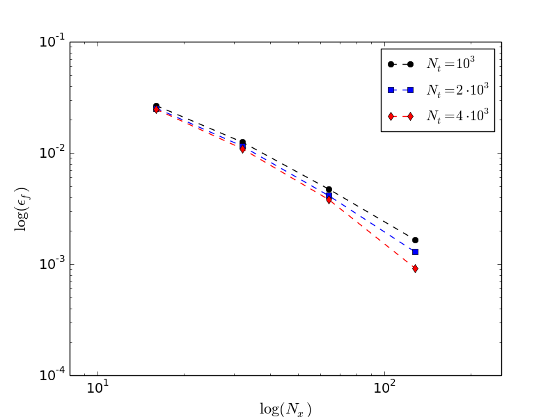
The final time of the evolution is . The initial condition has the following form:
| (43) | |||
| (44) | |||
| (45) |
where and . A mixed discretization is considered, namely a spectral collocation method for the space and standard centered finite differences in velocity. The contour plot of the reference solution at final time is shown in Figure 3. The conservation properties and the errors with respect to a reference simulation are investigated by varying the phase space discretization as well as time step and the residual tolerance. The results are very similar to the ones obtained for the linear Landau damping testcase. For the sake of brevity, the conservation error properties are not reported. The errors with respect to a reference simulation () are computed by varying the discretization of the phase space and the time step. In particular, ranges in , and . The tolerance on the residual is varied and the errors when considering are shown in Figure 3. A second order convergence rate is retrieved for the space discretization, at fixed time step. Whereas the error is relatively insensitive to the time step when a coarse discretization is considered, a definite dependence is seen for the finest grid resolution. This is due to the fact that, on the coarse grids, the discretization error is dominated by the space discretization error.
5.3 2D-2D simulations
In this section, we present a 2D-2D Landau damping test case. The simulation domains are and . We impose as before periodic boundary conditions on and homogeneous Dirichlet boundary conditions on . Uniform tensor discretizations are used for and , and two different simulations are obtained for the following numbers of degrees of freedom: . The error tolerance criterion of the algorithm is set to be . Time step is equal to .
The initial condition is defined as
where and .
The evolution of the electric energy as a function of time is shown in Figure 4 for the two different discretizations mentioned above. It can be seen that these are in agreement with the predicted analytical decay. Conservation properties of mass, momentum and total energy behave similarly to 1D-1D cases. Ranks of the approximated solution obtained by the algorithm also seem to increase linearly with time.

We mention here that encouraging preliminary results have been obtained on 3D-3D test cases. Parallelisation of the method, which is needed to reduce the computational cost, is work in progress, and should enable to obtain results in more realistic settings.
6 Conclusion
In this work a dynamical adaptive tensor method has been proposed to build parsimonious discretizations for the Vlasov-Poisson system. It allows to treat generic geometries and can be applied to generic heterogeneous discretizations in space and velocity, making it a flexible tool for the simulation of kinetic equation within an Eulerian framework. The method is dynamical in time and the time advancing is design to preserve the Hamiltonian character of the system, with a second order accuracy. Several testcases were proposed to validate the method and assess its properties.
Several perspectives arise, concerning the parallelisation of the method (which is mandatory to deal with more realistic 3D-3D settings) and its extension to other kinetic equations, involving collision operators. These will be the object of a further investigation.
Appendix A: Proof of Proposition 2
Proof of Proposition 2.
Let us denote by the Riesz representative of b in . The element solution of (25) is then the unique solution to
where denotes the identity operator on . By assumption, , thus both (A1) or (A2) imply that . For all , let us denote by the residual of the equation in after iterations of the Fixed-point PGD algorithm. Since is solution to the minimization problem (26), it satisfies
| (46) |
Thus, we have the following properties on the tensor product function
| (47) | |||
| (48) | |||
We refer the reader to [31, 5, 18, 19, 20] for a proof of the properties (47), (48) and (48), which are consequences of (46). Let us already point out here that if (which is the case when assumption (A1) is satisfied), we have in addition
| (49) |
Thus, since ,
At this point, we treat the two cases separately. Let us first assume that (A1) holds. Then,
Assume now that (A2) holds. Then,
In both cases, there exists a constant such that
Thus, the sequence is non-increasing and converges. Since , and , this implies that is a bounded sequence in . Besides, the series is convergent, and . Up to the extraction of a subsequence (still denoted for the sake of simplicity), weakly converges in to some . Property (48) implies that
Since , we obtain that is necessarily equal to , the unique solution of (25). The sequence thus entirely converges (weakly) to in . The strong convergence can be obtained using the same arguments as in [5], which yields the desired result. ∎
References
- [1] Luigi Ambrosio, Maria Colombo, and Alessio Figalli. On the lagrangian structure of transport equations: the Vlasov-Poisson system. arXiv preprint arXiv:1412.3608, 2014.
- [2] Aleksei Alekseevich Arsenev. Existence in the large of a weak solution to the Vlasov system of equations. Zhurnal Vychislitelnoi Matematiki i Matematicheskoi Fiziki, 15:136–147, 1975.
- [3] Claude Bardos and Pierre Degond. Global existence for the Vlasov-Poisson equation in 3 space variables with small initial data. In Annales de l’IHP Analyse non linéaire, volume 2, pages 101–118, 1985.
- [4] JU Brackbill. On energy and momentum conservation in particle-in-cell plasma simulation. Journal of Computational Physics, 317:405–427, 2016.
- [5] Eric Cances, Virginie Ehrlacher, and Tony Lelievre. Convergence of a greedy algorithm for high-dimensional convex nonlinear problems. Mathematical Models and Methods in Applied Sciences, 21(12):2433–2467, 2011.
- [6] Eric Cances, Virginie Ehrlacher, and Tony Lelievre. Greedy algorithms for high-dimensional non-symmetric linear problems. In ESAIM: Proceedings, volume 41, pages 95–131. EDP Sciences, 2013.
- [7] Fernando Casas, Nicolas Crouseilles, Erwan Faou, and Michel Mehrenberger. High-order hamiltonian splitting for Vlasov-Poisson equations. arXiv preprint arXiv:1510.01841, 2015.
- [8] Paul Cazeaux and Jan S Hesthaven. Multiscale time-integration for particle-in-cell methods. Technical report, Elsevier, 2014.
- [9] Frédérique Charles, Bruno Després, and Michel Mehrenberger. Enhanced convergence estimates for semi-lagrangian schemes application to the Vlasov–Poisson equation. SIAM Journal on Numerical Analysis, 51(2):840–863, 2013.
- [10] Francisco Chinesta, Amine Ammar, and Elías Cueto. Recent advances and new challenges in the use of the proper generalized decomposition for solving multidimensional models. Archives of Computational methods in Engineering, 17(4):327–350, 2010.
- [11] Francisco Chinesta, Pierre Ladeveze, and Elías Cueto. A short review on model order reduction based on proper generalized decomposition. Archives of Computational Methods in Engineering, 18(4):395–404, 2011.
- [12] H Cho, D Venturi, and GE Karniadakis. Numerical methods for high-dimensional probability density function equations. Journal of Computational Physics, 305:817–837, 2016.
- [13] Nicolas Crouseilles, Guillaume Latu, and Eric Sonnendrücker. A parallel Vlasov solver based on local cubic spline interpolation on patches. Journal of Computational Physics, 228(5):1429–1446, 2009.
- [14] Nicolas Crouseilles, Michel Mehrenberger, and Eric Sonnendrücker. Conservative semi-lagrangian schemes for Vlasov equations. Journal of Computational Physics, 229(6):1927–1953, 2010.
- [15] Pierre Degond, Lorenzo Pareschi, and Giovanni Russo. Modeling and computational methods for kinetic equations. Springer Science & Business Media, 2004.
- [16] Laurent Desvillettes and Jean Dolbeault. On long time asymptotics of the Vlasov—Poisson—Boltzmann equation. Communications in partial differential equations, 16(2-3):451–489, 1991.
- [17] Mike Espig and Aram Khachatryan. Convergence of alternating least squares optimisation for rank-one approximation to high order tensors. arXiv preprint arXiv:1503.05431, 2015.
- [18] Antonio Falco and Anthony Nouy. A proper generalized decomposition for the solution of elliptic problems in abstract form by using a functional eckart–young approach. Journal of Mathematical Analysis and Applications, 376(2):469–480, 2011.
- [19] Antonio Falcó and Anthony Nouy. Proper generalized decomposition for nonlinear convex problems in tensor banach spaces. Numerische Mathematik, 121(3):503–530, 2012.
- [20] Leonardo E Figueroa and Endre Süli. Greedy approximation of high-dimensional Ornstein–Uhlenbeck operators. Foundations of Computational Mathematics, 12(5):573–623, 2012.
- [21] Francis Filbet and Eric Sonnendrücker. Comparison of eulerian vlasov solvers. Computer Physics Communications, 150(3):247–266, 2003.
- [22] Kai Germaschewski, William Fox, Stephen Abbott, Narges Ahmadi, Kristofor Maynard, Liang Wang, Hartmut Ruhl, and Amitava Bhattacharjee. The plasma simulation code: A modern particle-in-cell code with patch-based load-balancing. Journal of Computational Physics, 318:305–326, 2016.
- [23] Robert T Glassey. The Cauchy problem in kinetic theory. SIAM, 1996.
- [24] Alexandre Grothendieck. Résumé de la théorie métrique des produits tensoriels topologiques. Resenhas do Instituto de Matemática e Estatística da Universidade de São Paulo, 2(4):401–481, 1996.
- [25] Wolfgang Hackbusch, Boris N Khoromskij, and Eugene E Tyrtyshnikov. Approximate iterations for structured matrices. Numerische Mathematik, 109(3):365–383, 2008.
- [26] Ernst Hairer, Christian Lubich, and Gerhard Wanner. Geometric numerical integration illustrated by the Störmer–Verlet method. Acta numerica, 12:399–450, 2003.
- [27] Ernst Hairer, Christian Lubich, and Gerhard Wanner. Geometric numerical integration: structure-preserving algorithms for ordinary differential equations, volume 31. Springer Science & Business Media, 2006.
- [28] Hyung Ju Hwang. Regularity for the Vlasov–Poisson system in a convex domain. SIAM journal on mathematical analysis, 36(1):121–171, 2004.
- [29] Katharina Kormann. A semi-lagrangian Vlasov solver in tensor train format. SIAM Journal on Scientific Computing, 37(4):B613–B632, 2015.
- [30] Pierre Ladeveze, J-C Passieux, and David Néron. The latin multiscale computational method and the proper generalized decomposition. Computer Methods in Applied Mechanics and Engineering, 199(21):1287–1296, 2010.
- [31] Claude Le Bris, Tony Lelievre, and Yvon Maday. Results and questions on a nonlinear approximation approach for solving high-dimensional partial differential equations. Constructive Approximation, 30(3):621–651, 2009.
- [32] PIERRE-LOUIS Lions and BENOˆIT Perthame. Propagation of moments and regularity for the 3-dimensional Vlasov-Poisson system. Inventiones mathematicae, 105(1):415–430, 1991.
- [33] Éric Madaule, Marco Restelli, and Eric Sonnendrücker. Energy conserving discontinuous Galerkin spectral element method for the Vlasov–Poisson system. Journal of Computational Physics, 279:261–288, 2014.
- [34] Jerrold E. Marsden and Alan Weinstein. The hamiltonian structure of the Maxwell-Vlasov equations. Physica D: Nonlinear Phenomena, 4(3):394 – 406, 1982.
- [35] PJ Morrison. Hamiltonian and action principle formulations of plasma physicsa). Physics of Plasmas (1994-present), 12(5):058102, 2005.
- [36] Anthony Nouy. A priori model reduction through proper generalized decomposition for solving time-dependent partial differential equations. Computer Methods in Applied Mechanics and Engineering, 199(23):1603–1626, 2010.
- [37] Martin Campos Pinto and Michel Mehrenberger. Convergence of an adaptive semi-lagrangian scheme for the Vlasov-Poisson system. Numerische Mathematik, 108(3):407–444, 2008.
- [38] Thorsten Rohwedder and André Uschmajew. On local convergence of alternating schemes for optimization of convex problems in the tensor train format. SIAM Journal on Numerical Analysis, 51(2):1134–1162, 2013.
- [39] Vladimir N Temlyakov. Greedy approximation. Acta Numerica, 17:235–409, 2008.
- [40] André Uschmajew. Local convergence of the alternating least squares algorithm for canonical tensor approximation. SIAM Journal on Matrix Analysis and Applications, 33(2):639–652, 2012.
- [41] Victor Vedenyapin, Alexander Sinitsyn, and Eugene Dulov. Kinetic Boltzmann, Vlasov and Related Equations. Elsevier, 2011.
- [42] Xingyu Wang, Roman Samulyak, Xiangmin Jiao, and Kwangmin Yu. AP-Cloud: Adaptive Particle-in-Cloud method for optimal solutions to Vlasov–Poisson equation. Journal of Computational Physics, 316:682–699, 2016.
- [43] Jin Xu, Peter N Ostroumov, Brahim Mustapha, and Jerry Nolen. Scalable direct vlasov solver with discontinuous galerkin method on unstructured mesh. SIAM Journal on Scientific Computing, 32(6):3476–3494, 2010.