Supersymmetric black lenses in five dimensions
Abstract
We present an asymptotically flat supersymmetric black lens solution with the horizon topology in the five-dimensional minimal ungauged supergravity. We show that the black lens carries a mass, two independent angular momenta, electric charge and magnetic fluxes, among which only the quantities are independent.
pacs
04.50.+h 04.70.BwI Introduction
Black hole solutions to Einstein’s equations have provided an excellent arena to test a number of classical and quantum aspects of gravity. In particular, higher dimensional black holes have attracted much attention in last two decades, for instance by the microscopic derivation of Bekenstein-Hawking entropy [1] and the realistic production of black holes at accelerators in the scenario of large extra dimensions [2]. In spite of startling developments for higher-dimensional black holes, our understanding of higher dimensional gravity is still poor since it is much richer and captures more degree of freedom. According to the topology theorem of a stationary black hole in five dimensions [3, 4], the allowed topology of the cross section of the event horizon is restricted either to a sphere , a ring or lens spaces , provided the spacetime is asymptotically flat and allows two commuting axial Killing vector fields (more generally, the cross section of the stationary horizon must be of positive Yamabe-type under the dominant energy condition [6, 5]). In the first two cases, we have the corresponding exact solutions to vacuum Einstein’s equations [7, 8, 9, 10]. In contrast, a vacuum black hole solution with the lens space topology turns out difficult to come by and is still missing.11 1 Although the vacuum black-hole solution constructed in [11] has a lens space topology , it is not asymptotically flat since the spatial section at infinity has a ‘flipped’ lens topology . Exploiting the inverse scattering method, several authors tried to find an asymptotically flat solution to the five-dimensional vacuum Einstein equations, but unfortunately all of these attempts failed [12, 13]. A major obstacle in the construction of a black lens is that the resultant solutions are always plagued by naked singularities.
Recently, an asymptotically flat supersymmetric black lens solution with the topology has been constructed by Kunduri and Lucietti [14] in the framework of the five-dimensional minimal ungauged supergravity (see [15] for the extension to supergravity). The construction relies heavily on the machinery developed by Gauntlett et. al [16]. In that paper, they generalized the earlier program in [17] into higher dimensions and demonstrated that the supersymmetric solutions can be systematically classified by using bilinears built out of the Killing spinor. These bilinears define a previledged -structures, which tightly constrain the possible forms of the metric and the gauge fields [19, 20]. It turns out that the metric of supersymmetric solutions admitting a timelike bilinear Killing field is described in an adapted coordinate system by an -bundle over the 4-dimensional hyper-Kähler base space and the governing equations are linear, allowing us to find a number of exact solutions of physical interest. The program undertaken in [16] has replaced the standard ansatz-based approaches and provoked a drastic progress in classifications of BPS solutions with various fractions of supersymmetry in diverse supergravities [21, 22, 23, 24, 25, 26, 27, 28, 29, 30, 31, 32, 33]. An alternative approach referred to as a spinorial geometry also gives us an elegant and powerful method for classifying supergravity solutions (see [34, 35, 36, 37, 38, 39, 40, 41] for an incomplete list of references). These domains of research have been motivated by the desire to figure out the string duality and the gauge/gravity correspondence.
For the supersymmetric black objects in asymptotically flat spacetimes in the five-dimensional minimal supergravity, a number of properties have been clarified by many authors. The most salient feature of a supersymmetric black hole is that the horizon must be degenerate and non-rotating. This is because the bilinear Killing vector becomes never spacelike, and hence the ergoregion does not exist [42]. Reall gave a proof that the possible topologies of the supersymmetric black holes are either , , or quotient thereof [43]. For the first case, Breckenridge et al. constructed a black hole with a spherical topology admitting angular momenta [44], referred to as a BMPV black hole. The BMPV black hole is characterized by the mass and two equal angular momenta, due to which the spatial symmetry is enhanced to [45]. As in the Kerr case, the magnitude of angular momentum is bounded by the mass, otherwise a naked time machine shows up. The second possibility corresponding to a black hole with a ring topology has been found in [46]. The black ring enjoys only the spatial symmetry and precludes a configuration with equal angular momenta, which distinguish it from the BMPV black hole. The angular momentum along the direction does not have an upper bound, in sharp contrast to the spherical counterpart. A more intriguing feature arises in the supergravity, where the three-charge black ring is specified by 7 parameters, while only 5 of them are conserved quantities [47, 48]. This exhibits a classical infinite non-uniqueness of black objects.
Ref. [43] also proved that the only asymptotically flat black-hole solution to five-dimensional minimal supergravity whose near-horizon geometry is locally isometric to that of BMPV black hole is the BMPV black hole, provided that the bilinear Killing field is everywhere timelike outside the Killing horizon. The black lens space found in [14] does not counter to the above uniqueness theorem, since the bilinear Killing field happens to be null at some points outside the horizon. These “critical surfaces” or “evanescent ergosurfaces” [54] are regular timelike surfaces and provide us with much richer varieties of black holes. For instance, ref. [55] pointed out that the black hole with a spherical topology other than the BMPV solution indeed exists. Another interesting facet of a black lens in [14] and the solution in [55] is that they have nontrivial 2-cycles outside the horizon. This kind of “bubbling” solutions is of crucial importance in the context of fuzzball conjectures [49], and a number of solitons and black holes/rings with bubbles have been found [50, 51, 52, 53]. A key ingredient to bring about these bubbles is that the spatial hypersurface has nontrivial second homology class, which is not realizable in four dimensions.
In this paper, we generalize the work of Kunduri and Lucietti [14] to the more general lens space, and construct an asymptotically flat supersymmetric black lens solution with the horizon topology of for in the five-dimensional minimal ungauged supergravity. The regular metric on the lens space with unit radius can be written as
| (1) |
where , and . The parameter is an integer parametrizing the Chern class of the principal bundle over . In particular, this reduces to a metric on a three-dimensional sphere for written in terms of the Euler angle coordinates. Our strategy is to consider the Gibbons-Hawking space as a hyper-Kähler base space and allow the harmonic functions to have point sources with appropriate coefficients. By imposing suitable boundary conditions, we find the configuration in which the cross section of the horizon becomes and the cross section of null infinity becomes . Our black lens solution possesses nontrivial 2-cycles supported by magnetic fluxes outside the horizon. One of them touches the horizon and forms the disk topology, while others are away from the horizon.
We organize the present paper as follows. In the next section II, we present the supersymmetric solutions describing black lenses in the five-dimensional minimal ungauged supergravity. The solution is stationary and bi-axially symmetric admitting isometry. In section III, we study in depth the boundary conditions under which the spacetime is asymptotically flat, no closed timelike curves (CTCs) appear around the horizon, no (conical and curvature) singularities develop in the domain of outer communications, and no orbifold singularities nor Dirac-Misner strings exist on the axis. This boundary conditions place restrictions upon the parameters and it turns out that the physical solution is specified by parameters. Section IV analyzes some physical properties of black lenses. This includes the discussion about conserved quantities and CTCs. In the final section V, we devote ourselves to the summary and discussion on our results.
II Black lens solution
Let us begin with a basic setup for supersymmetric solutions in the five-dimensional minimal ungauged supergravity, whose bosonic Lagrangian consists of the Einstein-Maxwell theory with a Chern-Simons term and takes the form [56]
| (2) |
where is the Maxwell field. The gravitational solution is said to be supersymmetric if it admits a spinor obeying the first-order differential equations
| (3) |
The supersymmetric solutions to five-dimensional minimal ungauged supergravity have been systematically classified according to the causal nature of the Killing vector constructed out of the Killing spinor [16]. In the domain where is timelike, the local metric and the gauge field strength have a simple description in the -independent form
| (4) | |||||
| (5) |
where and is the metric of a hyper-Kähler base space. The norm and the twist of a Killing vector are a scalar and a 1-form on the base space and obey a linear system
| (6) |
where we have employed a convention that the hypercomplex structures are anti-self-dual. If this system is solved, the solution to the Killing spinor equation (3) is given by , where is a covariantly constant chiral Killing spinor of the hyper-Kähler base space, i.e., the solution preserves at least half of supersymmetries.
Among a variety of hyper-Kähler spaces, the Gibbons-Hawking space [57] plays a distinguished role. The metric of the Gibbons-Hawking space reads
| (7) |
where are Cartesian coordinates on and is a triholomorphic Killing vector. When continues a symmetry generator for the five-dimensional metric and the gauge field , it commutes with and the supersymmetry-preserving dimensional reduction is possible.22 2 When the Kaluza-Klein Killing vector fails to commute with the supersymmetric Killing vector, the dimensional reduction breaks supersymmetry. See [58] for a notable example. Furthermore, every bosonic element can be obtained in a closed form and reads [16, 60]
| (8) | |||||
| (9) | |||||
| (10) | |||||
| (11) | |||||
| (12) |
which leads to
| (13) |
Here are harmonic functions on , which are only the necessary input to specify the supersymmetric solutions. It should be observed that there exists a gauge freedom of redefining harmonic functions [62]
| (14) |
where is a constant. Under (14), one can easily verify that () remain invariant, whereas the 1-form undergoes a change as . Since this transformation merely amounts to the gauge transformation , the transformation (14) makes the bosonic sector invariant. We shall come back to this freedom (14) in the following analysis.
When the general choice of these harmonics are made, the solution fails to be asymptotically flat or suffers from CTCs, and the existence of the horizon is not guaranteed. Following the paper by Kunduri and Lucietti [14] (see also [59]), we consider the following class of harmonic functions
| (15) | |||||
| (16) | |||||
| (17) | |||||
| (18) |
Here, , where are constants. This choice of harmonics reduces to that of the BMPV black hole [44] for , and that of the black lens with for [14].
The 1-forms () are obtained by
| (19) | |||||
| (20) | |||||
| (21) |
where 1-forms and () on are defined by (c.f [61]).
| (22) | |||||
| (23) |
where are constants.33 3 One can also add pure-gradient terms to . However, the regularity of the solution requires that these additional constants must vanish in the present context. These 1-forms satisfy and . Throughout this paper, we set for all (in this case is another Killing field) and assume for . In this case, and are simplified in spherical coordinates () to
| (24) | |||||
| (25) |
with the constant
| (26) |
where . Obviously, we have a freedom to choose , which can be used to set without losing any generality.
Under the transformation (14), the coefficient of term in varies as . It therefore turns out that an appropriate choice of allows us to set
| (27) |
Hence, the solution contains parameters (). We shall see below that the regular boundary conditions constrain some of them and the physical solution is specified only by parameters.
III Boundary conditions
In order to obtain a supersymmetric black lens solution of physical interest, we impose suitable boundary conditions at (i) infinity, (ii) horizon , (iii) “bubbles” and (iv) axis . The boundary condition at infinity (i) must be such that the spacetime is asymptotically flat. At the horizon (ii), the surface should correspond to a smooth degenerate null surface whose spatial cross section has a topology of the lens space . At the points (iii) where each harmonic function diverges, we put constraints upon parameters in such a way that these points correspond merely to the coordinate singularities like the origin of the Minkowski spacetime. On the axis, we demand that there appear no Dirac-Misner strings, and orbifold singularities at isolated points must be eliminated. At these boundaries, the spacetime is required to allow neither CTCs nor (conical and curvature) singularities.
III.1 Infinity
Let us begin by addressing the asymptotic flatness of the solution. For , the metric functions () behave as
| (28) |
Since the 1-forms and are approximated by
| (29) |
one gets
| (30) | |||||
| (31) | |||||
The asymptotic flatness demands the parameters to satisfy
| (32) | |||||
| (33) | |||||
| (34) |
In terms of the radial coordinate , the metric asymptotically () approaches to
| (35) |
This is nothing but the metric of Minkowski spacetime for which the corresponding to the cross section of spatial infinity is written in terms of Euler angles (. The avoidance of conical singularities requires the range of angles to be , and with the identification and .
III.2 Horizon
We next show that the point source corresponds to a degenerate Killing horizon and the topology of the spatial cross section is a lens space . Since we have imposed , we now look at the behavior of the solution around the origin . Since four harmonic functions , , and are expanded as
| (36) |
the functions and reduce to
| (37) |
Here we have defined the constants and by
| (38) | |||||
| (39) | |||||
The -forms and are
| (40) | |||
| (41) |
yielding
| (42) | |||||
and
| (43) |
In terms of new coordinates given by
| (44) |
we wish to require that the metric is regular around . A potential divergence appears from and , which can be eliminated by
| (45) | |||||
| (46) | |||||
| (47) | |||||
With this choice, it turns out that the metric is then analytic in and therefore can be extended into the region. It follows that the null surface corresponds to the Killing horizon for the supersymmetric Killing field .
Taking the higher-order terms in into account, one obtains the near-horizon limit by and [43]. After some algebra, one arrives at
| (48) | |||||
and
| (49) |
where we have defined
| (50) | |||
| (51) |
This is locally isometric to the near-horizon geometry of the BMPV black hole [63, 42].44 4 In spite of this, one can verify that the metric (48) with (49) preserves the maximal amount of supersymmetry, as in the near-horizon geometry of the BMPV black hole. This is quite nontrivial because the discrete identification in general breaks supersymmetry. The primary reason for this is that is a symmetry of two independent Killing spinors. This can be demonstrated by a direct integration of the Killing spinor equations (3). In order to remove CTCs around the horizon, one requires and , which simply amounts to the inequality
| (52) |
III.3 Bubbles ()
There exists apparent divergence in the metric of the Gibbons-Hawking space at the points (). We shall impose the boundary conditions at each point () that this corresponds to a smooth point analogous to the origin of Minkowski spacetime, rather than horizons. To demonstrate this, let us choose the coordinates on of the Gibbons-Hawking space so that the -th point () is an origin of . Near the origin , the four harmonic functions , , and behave as
| (54) | |||||
| (55) |
yielding
| (56) |
where the constants and are defined by
| (57) | |||||
| (58) |
The 1-forms and are approximated by
| (59) | |||
| (60) |
giving rise to
| (61) |
where
| (62) | |||||
| (63) | |||||
| (64) |
One therefore obtains the asymptotic behavior of the metric around the -th point as
| (65) | |||||
As a minimal requirement, we impose the following conditions on the parameters :
| (66) | |||||
| (67) |
which implies
| (68) |
Hence, (66) and (67) are sufficient to get rid of divergence in and ensure that no curvature singularities appear in the domain of outer communications. Converting to the new coordinates by
| (69) |
one verifies that the metric near reduces to
| (70) |
To ensure the metric the Lorentzian signature, one needs
| (71) |
Although (70) is locally isometric to the flat space metric, necessarily becomes timelike and CTCs appear, because we are now focusing on the region . To remove this causal violation around each , it suffices to impose at (), which in the present case rehashes to
| (72) |
These conditions are obtained by requiring at () and referred to as “bubble equations” in refs [53, 49]. These bubbles describe the timelike and regular surfaces. The bubble equations account for the delicate balance between the gravitational attraction and the repulsion by flux through the cycles.
There still remains a possibility of CTCs associated with a vector field with closed orbits remains spacelike (note that is integer). Quite amazingly, is automatically satisfied for all , if we impose (72). We relegate the proof of this in Appendix A. It follows that no causal violation occurs around each bubble if one demands (72).
III.4 Axis
The -axis of (i.e., ) in the Gibbons-Hawking space splits up into the intervals: , and . On the -axis, the -forms and are, respectively, simplified to
| (73) |
In particular, on , and become, respectively,
| (74) |
Hence, on , vanishes since
| (75) | |||||
where we have used Eq. (34) at the last equality.
On the interval , one computes
| (76) | |||||
where we have used Eq. (105). Finally for we get
| (77) | |||||
where we have used Eq. (104). Since (see Appendix A), one concludes (i.e., ) on for . It therefore turns out that holds at each interval. This proves that no Dirac-Misner string pathologies happen throughout the spacetime. As argued in [49, 54], the absence of the Dirac-Misner string among each bubble is a direct consequence of the bubble equations (72). However, at seems quite nontrivial.
Let us next move onto the discussion of the issue of orbifold singularities. On we get
| (78) |
whereas on we have
| (79) | |||||
Accordingly, the two-dimensional -part of the metric on the intervals and can be written in the form
| (80) |
In the analysis of orbifold singularities, it is more advantageous to work in the coordinate basis vectors of periodicity, instead of , where these coordinates are defined by and . From (80), one sees that the Killing vector vanishes on each interval. More precisely, one sees that
- •
on the interval , the Killing vector vanishes,
- •
on each interval (), the Killing vector vanishes,
- •
on the interval , the Killing vector vanishes.
From these, we can observe that the Killing vectors on the intervals satisfy
| (81) |
with
| (82) |
Eq. (81) assures that the metric smoothly joints at the end points of the intervals [3], which means that there exist no orbifold singularities at adjacent intervals. Furthermore, eq. (82) illustrates that the horizon cross section is topologically the lens space .
III.5 Summary of boundary conditions
The regularity of the metric at each boundary has requested us to impose the conditions (32), (33), (34), (66), (67) and (72). Combined with , this reduces the independent parameters of the solution from to . Moreover, these parameters are subject to the constraints (52) and (71). The latter condition boils down to
| (83) |
IV Physical properties
As appropriate boundary conditions are prescribed in the last section, let us now investigate several physical properties of the solution.
IV.1 Conserved quantities
Let us discuss conserved quantities of the black lens solution. As shown in section III.1, the spacetime is asymptotically flat, which enables us to ADM mass the ADM mass and two ADM angular momenta as
| (84) | |||||
| (85) | |||||
| (86) |
where is the electric charge normalized by (note that the Chern-Simons term fail to contribute)
| (87) |
It follows that the Bogomol’ny bound is saturated [64]. In appearance, the positivity of the ADM mass is not obvious from the above expressions. Nevertheless, one can establish the positivity of the mass by using the relations (50) and (66) as
| (88) | |||||
where we have used the inequality (50).
The surface gravity and the angular velocities of the horizon vanish, as expected for supersymmetric black objects in the asymptotically flat spacetime [42]. The area of the horizon is nonvanishing and reads from (48) as
| (89) |
The interval has a disc topology and the intervals () is a two-dimensional sphere, respectively. The magnetic fluxes through are defined as
| (90) |
Since the Maxwell gauge field is smooth at the horizon, bubbles and critical surfaces, one can evaluate these fluxes as , which are computed to give55 5 Perhaps, ref. [14] misses the contribution coming from the horizon.
| (91) |
An alternative definition of magnetic flux proposed in [49] is
| (92) |
This definition does not apply in the present setting, because diverges at the critical surfaces at which . The interval corresponds to the disk topology surface ending on the horizon, whereas the intervals () represents 2-cycles (or bubbles) outside the horizon.
When , , all magnetic fluxes vanish. Under this parameter-setting, the condition (83) can be simply written as
| (93) |
However, it turns out that these inequalities cannot be satisfied, since the left-hand side is non-positive by (52) while the right-hand side is positive by our assumption. As for the supersymmetric solutions which we have obtained, one may therefore interpret that the horizon of the lens space topology must be supported by the magnetic fluxes.
When
| (94) |
the angular momentum vanishes, which implies that the black lens has equal angular momenta as the BMPV black hole does. For , the inequality (83) is never satisfied in the choice of the parameters (94), which means that the black lens with equal angular momenta cannot be realized [14]. For , it seems impracticable to show this claim analytically. As far as we checked numerically for , we find no parameter regions under which the configuration of equal angular momenta is realized. We expect that this situation does not change for , and our family of black lenses does not admit equal angular momenta.
IV.2 No CTCs
We wish to impose that the domain of outer communication in the five-dimensional spacetime remains Lorenzian without CTCs. This amounts to
| (95) |
These conditions ensure that is a global timelike coordinate and the spacetime is stably causal. Explicitly, these conditions boil down to
| (96) | ||||
| (97) | ||||
| (98) |
It is considerably elaborate to check their positivity. For instance, one finds
| (99) |
where we have used (83). Due to the triangle inequality , we find that the first term in the summation of the right-hand side is non-negative, while the second term is rewritten into
| (100) |
where we used . This term vanishes for , whereas its positivity is unclear for .
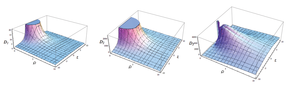
Nevertheless, we made substantial numerical scans for the positivity of ’s and found that there appear no causal violations in the domain of outer communications (see Fig. 1). We expect that (52) and (83) are sufficient to remove causal pathologies on and outside the horizon.
IV.3 Critical surfaces
A key issue for the construction of the black lens is the contrived choice of harmonic functions (15)–(18). One immediate notable feature is that is negative around (), giving rise to the () signature of the Gibbons-Hawking base space. This is not problematic as long as remains positive. There appear “critical surfaces” [49] at which corresponding to . From the five-dimensional point of view, this is called an “evanescent ergosurface” [54, 66]. This is not problematic since these surfaces exist also in [54].
The existence of critical surfaces provokes a striking impact on the uniqueness theorems of supersymmetric black hole. In the original proof [43], it has been assumed that the supersymmetric Killing field is strictly timelike outside the horizon. Recently it has been pointed out in [55] that these critical surfaces can get around the uniqueness theorems. Since the topologically nontrivial cycles run between two point sources for the Gibbons-Hawking harmonic function, this way of avoiding uniqueness theorems does not happen in four dimensions.
At these regularity surfaces, one must impose the regularity condition when . Namely, if there exist points on the axis such that
| (101) |
these critical surfaces are singular. In case, this does not occur by the restriction (83), whereas the case seems nontrivial, although we have not found the singular behavior numerically. If these surfaces were singular, (101) gives rise to
| (102) |
Hence, a sufficient condition to avoid the singularity at critical surfaces is
| (103) |
V Summary
In this work, we have constructed an asymptotically flat supersymmetric black lens solution in the bosonic sector of the five-dimensional minimal supergravity, whose horizon topology is a lens space of (). This represents a generalization of the solution found in [14]. We also computed the conserved charges including the (positive and BPS-saturating) mass, two angular momenta, and magnetic fluxes, among which quantities are independent.
As is concerned with the black lens solution which we have obtained in this work, there exists no limit such that all the magnetic fluxes vanish. Therefore, as for the supersymmetric solutions, the existence of the magnetic fluxes seem to play an essential role in supporting the horizon of the black lens. In general, however, it is not clear whether one necessarily needs such magnetic fluxes in order to construct a black lens.
It appears straightforward to generalize the present work to into supergravity and uplift the solution into 11 dimensions [47]. Performing the Kaluza-Klein reduction and the subsequent T-dualities, the solution can be converted into the D1-D5-P system. We expect that a decoupling limit can be taken as in the case, which would enable us to exploit Cardy formula to reproduce the Bekenstein-Hawking entropy.
In this line of research, one of the most exciting generalizations might be to look for a non-supersymmetric black lens. Such a black lens, if they exist, in particular a vacuum solution, must differ considerably from the solutions presented here, since we have mede use of the flux threading the 2-cycles to prevent the collapse, while in the vacuum case this does not occur [54].
Acknowledgements.
This work was partially supported by the Grant-in-Aid for Young Scientists (B) (No. 26800120) from Japan Society for the Promotion of Science (S.T.), and by MEXT Grant-in-Aid for Scientific Research on Innovative Areas“New Developments in Astrophysics Through Multi-Messenger Observations of Gravitational Wave Sources” (Grant Number A05 24103006) (M.N).Appendix A Proof of
At each bubble, no causal violation requires that holds for . To prove this is the main result of the present appendix. Let us note that from (66) and (67), the bubble equations (72) can be written as
| (104) | |||||
The summation of (104) for gives
| (105) | |||||
where the last term in the first line vanishes by the antisymmetry for and . From Eqs. (66) and (67), is written as
| (106) | |||||
The third, fifth and sixth terms of the right-hand side of (106) are combined into
| (107) |
where we have used Eq. (104). Next, the summation of the first, second and fourth terms on the right-hand side of (106) reduces to
| (108) | |||||
where we we have used Eq. (104). After some lengthy, but straightforward computations, one can verify that (108) is further simplified to (107) up to the minus sign. This proves , as we desired to show.
References
- [1] A. Strominger and C. Vafa, “Microscopic origin of the Bekenstein-Hawking entropy,” Phys. Lett. B 379, 99 (1996) [hep-th/9601029].
- [2] P. C. Argyres, S. Dimopoulos and J. March-Russell, “Black holes and submillimeter dimensions,” Phys. Lett. B 441, 96 (1998) [hep-th/9808138].
- [3] S. Hollands and S. Yazadjiev, “Uniqueness theorem for 5-dimensional black holes with two axial Killing fields,” Commun. Math. Phys. 283, 749 (2008) [arXiv:0707.2775 [gr-qc]].
- [4] S. Hollands, J. Holland and A. Ishibashi, “Further restrictions on the topology of stationary black holes in five dimensions,” Annales Henri Poincare 12, 279 (2011) [arXiv:1002.0490 [gr-qc]].
- [5] M. l. Cai and G. J. Galloway, “On the Topology and area of higher dimensional black holes,” Class. Quant. Grav. 18, 2707 (2001) [hep-th/0102149].
- [6] G. J. Galloway and R. Schoen, “A Generalization of Hawking’s black hole topology theorem to higher dimensions,” Commun. Math. Phys. 266, 571 (2006) [gr-qc/0509107].
- [7] F. R. Tangherlini, “Schwarzschild field in n dimensions and the dimensionality of space problem,” Nuovo Cim. 27, 636 (1963).
- [8] R. C. Myers and M. J. Perry, “Black Holes in Higher Dimensional Space-Times,” Annals Phys. 172, 304 (1986).
- [9] R. Emparan and H. S. Reall, “A Rotating black ring solution in five-dimensions,” Phys. Rev. Lett. 88, 101101 (2002) [hep-th/0110260].
- [10] A. A. Pomeransky and R. A. Sen’kov, “Black ring with two angular momenta,” hep-th/0612005.
- [11] H. Lu, J. Mei and C. N. Pope, “New Black Holes in Five Dimensions,” Nucl. Phys. B 806, 436 (2009) [arXiv:0804.1152 [hep-th]].
- [12] J. Evslin, “Geometric Engineering 5d Black Holes with Rod Diagrams,” JHEP 0809, 004 (2008) [arXiv:0806.3389 [hep-th]].
- [13] Y. Chen and E. Teo, “A Rotating black lens solution in five dimensions”, Phys. Rev. D 78, 064062 (2008).
- [14] H. K. Kunduri and J. Lucietti,“Supersymmetric Black Holes with Lens-Space Topology”, Phys. Rev. Lett. 113, no. 21, 211101 (2014).
- [15] H. K. Kunduri and J. Lucietti, “Black lenses in string theory,” arXiv:1605.01545 [hep-th].
- [16] J. P. Gauntlett, J. B. Gutowski, C. M. Hull, S. Pakis and H. S. Reall, “All supersymmetric solutions of minimal supergravity in five- dimensions,” Class. Quant. Grav. 20, 4587 (2003) [hep-th/0209114].
- [17] K. p. Tod, “All Metrics Admitting Supercovariantly Constant Spinors,” Phys. Lett. B 121, 241 (1983).
- [18] J. P. Gauntlett and J. B. Gutowski, “All supersymmetric solutions of minimal gauged supergravity in five dimensions,” Phys. Rev. D 68 (2003) 105009 [Erratum-ibid. D 70 (2004) 089901] [hep-th/0304064].
- [19] J. P. Gauntlett, N. Kim, D. Martelli and D. Waldram, “Five-branes wrapped on SLAG three-cycles and related geometry,” JHEP 0111 (2001) 018 [hep-th/0110034].
- [20] J. P. Gauntlett, D. Martelli, S. Pakis and D. Waldram, “G-structures and wrapped NS5-branes,” Commun. Math. Phys. 247 (2004) 421 [hep-th/0205050].
- [21] J. B. Gutowski and H. S. Reall, “General supersymmetric AdS5 black holes,” JHEP 0404 (2004) 048 [hep-th/0401129].
- [22] J. B. Gutowski and W. Sabra, “General supersymmetric solutions of five-dimensional supergravity,” JHEP 0510 (2005) 039 [hep-th/0505185].
- [23] J. Bellorín, P. Meessen and T. Ortín, “All the supersymmetric solutions of , ungauged supergravity,” JHEP 0701 (2007) 020 [hep-th/0610196].
- [24] J. Bellorín and T. Ortín, “Characterization of all the supersymmetric solutions of gauged , supergravity,” JHEP 0708 (2007) 096 [arXiv:0705.2567 [hep-th]].
- [25] J. B. Gutowski, D. Martelli and H. S. Reall, “All supersymmetric solutions of minimal supergravity in six dimensions,” Class. Quant. Grav. 20 (2003) 5049 [hep-th/0306235].
- [26] J. P. Gauntlett and S. Pakis, “The geometry of Killing spinors,” JHEP 0304 (2003) 039 [hep-th/0212008].
- [27] J. P. Gauntlett, J. B. Gutowski and S. Pakis, “The geometry of null Killing spinors,” JHEP 0312 (2003) 049 [hep-th/0311112].
- [28] M. M. Caldarelli and D. Klemm, “All supersymmetric solutions of , gauged supergravity,” JHEP 0309 (2003) 019 [hep-th/0307022].
- [29] J. Bellorín and T. Ortín, “All the supersymmetric configurations of , supergravity,” Nucl. Phys. B 726 (2005) 171 [hep-th/0506056].
- [30] P. Meessen, T. Ortín and S. Vaulà, “All the timelike supersymmetric solutions of all ungauged supergravities,” JHEP 1011 (2010) 072 [arXiv:1006.0239 [hep-th]].
- [31] P. Meessen and T. Ortín, “Supersymmetric solutions to gauged sugra: the full timelike shebang,” Nucl. Phys. B 863 (2012) 65 [arXiv:1204.0493 [hep-th]].
- [32] M. Nozawa, “On the Bogomol’nyi bound in Einstein-Maxwell-dilaton gravity,” Class. Quant. Grav. 28, 175013 (2011) doi:10.1088/0264-9381/28/17/175013 [arXiv:1011.0261 [hep-th]].
- [33] D. Klemm and M. Nozawa, “Geometry of Killing spinors in neutral signature,” Class. Quant. Grav. 32, no. 18, 185012 (2015) doi:10.1088/0264-9381/32/18/185012 [arXiv:1504.02710 [hep-th]].
- [34] U. Gran, J. Gutowski and G. Papadopoulos, “The spinorial geometry of supersymmetric IIB backgrounds,” Class. Quant. Grav. 22 (2005) 2453 [hep-th/0501177].
- [35] U. Gran, J. Gutowski, G. Papadopoulos and D. Roest, “Systematics of IIB spinorial geometry,” Class. Quant. Grav. 23 (2006) 1617 [hep-th/0507087].
- [36] S. L. Cacciatori, M. M. Caldarelli, D. Klemm, D. S. Mansi and D. Roest, “Geometry of four-dimensional Killing spinors,” JHEP 0707 (2007) 046 [arXiv:0704.0247 [hep-th]].
- [37] J. B. Gutowski and W. A. Sabra, “Half-supersymmetric solutions in five-dimensional supergravity,” JHEP 0712 (2007) 025 [Erratum-ibid. 1004 (2010) 042] [arXiv:0706.3147 [hep-th]].
- [38] J. Grover, J. B. Gutowski and W. Sabra, “Null half-supersymmetric solutions in five-dimensional supergravity,” JHEP 0810 (2008) 103 [arXiv:0802.0231 [hep-th]].
- [39] S. L. Cacciatori, D. Klemm, D. S. Mansi and E. Zorzan, “All timelike supersymmetric solutions of , gauged supergravity coupled to abelian vector multiplets,” JHEP 0805 (2008) 097 [arXiv:0804.0009 [hep-th]].
- [40] D. Klemm and E. Zorzan, “All null supersymmetric backgrounds of , gauged supergravity coupled to abelian vector multiplets,” Class. Quant. Grav. 26 (2009) 145018 [arXiv:0902.4186 [hep-th]].
- [41] D. Klemm and E. Zorzan, “The timelike half-supersymmetric backgrounds of , supergravity with Fayet-Iliopoulos gauging,” Phys. Rev. D 82 (2010) 045012 [arXiv:1003.2974 [hep-th]].
- [42] J. P. Gauntlett, R. C. Myers and P. K. Townsend, “Black holes of D = 5 supergravity,” Class. Quant. Grav. 16, 1 (1999) [hep-th/9810204].
- [43] H. S. Reall, “Higher dimensional black holes and supersymmetry,” Phys. Rev. D 68, 024024 (2003) Erratum: [Phys. Rev. D 70, 089902 (2004)] [hep-th/0211290].
- [44] J. C. Breckenridge, R. C. Myers, A. W. Peet and C. Vafa, “D-branes and spinning black holes,” Phys. Lett. B 391, 93 (1997) [hep-th/9602065].
- [45] G. W. Gibbons and C. A. R. Herdeiro, “Supersymmetric rotating black holes and causality violation,” Class. Quant. Grav. 16, 3619 (1999) [hep-th/9906098].
- [46] H. Elvang, R. Emparan, D. Mateos and H. S. Reall, “A Supersymmetric black ring,” Phys. Rev. Lett. 93, 211302 (2004) [hep-th/0407065].
- [47] H. Elvang, R. Emparan, D. Mateos and H. S. Reall, “Supersymmetric black rings and three-charge supertubes,” Phys. Rev. D 71, 024033 (2005) [hep-th/0408120].
- [48] I. Bena and N. P. Warner, “One ring to rule them all … and in the darkness bind them?,” Adv. Theor. Math. Phys. 9, no. 5, 667 (2005) [hep-th/0408106].
- [49] I. Bena and N. P. Warner, “Black holes, black rings and their microstates,” Lect. Notes Phys. 755, 1 (2008) [hep-th/0701216].
- [50] I. Bena, S. Giusto, C. Ruef and N. P. Warner, “A (Running) Bolt for New Reasons,” JHEP 0911, 089 (2009) [arXiv:0909.2559 [hep-th]].
- [51] G. Compere, K. Copsey, S. de Buyl and R. B. Mann, “Solitons in Five Dimensional Minimal Supergravity: Local Charge, Exotic Ergoregions, and Violations of the BPS Bound,” JHEP 0912, 047 (2009) [arXiv:0909.3289 [hep-th]].
- [52] N. Bobev and C. Ruef, “The Nuts and Bolts of Einstein-Maxwell Solutions,” JHEP 1001, 124 (2010) [arXiv:0912.0010 [hep-th]].
- [53] I. Bena and N. P. Warner, “Bubbling supertubes and foaming black holes,” Phys. Rev. D 74, 066001 (2006) [hep-th/0505166].
- [54] G. W. Gibbons and N. P. Warner, “Global structure of five-dimensional fuzzballs,” Class. Quant. Grav. 31, 025016 (2014) [arXiv:1305.0957 [hep-th]].
- [55] H. K. Kunduri and J. Lucietti, “Black hole non-uniqueness via spacetime topology in five dimensions,” JHEP 1410, 82 (2014) [arXiv:1407.8002 [hep-th]].
- [56] E. Cremmer, “Supergravities in 5 dimensions,” in Superspace and Supergravity edited by S. W. Hawking and M. Rocek (Cambridge: Cambridge University Press 1981).
- [57] G. W. Gibbons and S. W. Hawking, “Gravitational Multi - Instantons,” Phys. Lett. B 78, 430 (1978).
- [58] D. Klemm and M. Nozawa, “Black holes in an expanding universe and supersymmetry,” Phys. Lett. B 753, 110 (2016) [arXiv:1511.01949 [hep-th]].
- [59] P. M. Crichigno, F. Porri and S. Vandoren, “Bound states of spinning black holes in five dimensions,” arXiv:1603.09729 [hep-th].
- [60] J. P. Gauntlett and J. B. Gutowski, “Concentric black rings,” Phys. Rev. D 71, 025013 (2005) [hep-th/0408010].
- [61] M. Dunajski and S. A. Hartnoll, “Einstein-Maxwell gravitational instantons and five dimensional solitonic strings,” Class. Quant. Grav. 24, 1841 (2007) [hep-th/0610261].
- [62] I. Bena, P. Kraus and N. P. Warner, “Black rings in Taub-NUT,” Phys. Rev. D 72, 084019 (2005) [hep-th/0504142].
- [63] A. H. Chamseddine, S. Ferrara, G. W. Gibbons and R. Kallosh, “Enhancement of supersymmetry near 5-d black hole horizon,” Phys. Rev. D 55, 3647 (1997) [hep-th/9610155].
- [64] G. W. Gibbons, D. Kastor, L. A. J. London, P. K. Townsend and J. H. Traschen, “Supersymmetric selfgravitating solitons,” Nucl. Phys. B 416, 850 (1994) [hep-th/9310118].
- [65] H. K. Kunduri and J. Lucietti, “The first law of soliton and black hole mechanics in five dimensions,” Class. Quant. Grav. 31, no. 3, 032001 (2014) [arXiv:1310.4810 [hep-th]].
- [66] B. E. Niehoff and H. S. Reall, “Evanescent ergosurfaces and ambipolar hyperkähler metrics,” JHEP 1604, 130 (2016) [arXiv:1601.01898 [hep-th]].