跳到论文正文
W Papers独立论文阅读器 arXiv:1606.06561 论文正文 计算阅读时间 · 0%
引用这篇论文根据当前论文元数据生成,正式投稿前建议核对。


License: arXiv.org perpetual non-exclusive license
arXiv:1606.06561v1 [gr-qc] 21 Jun 2016

Coherent 3jj-symbol representation for the loop quantum gravity intertwiner space

E. Alesci1, J. Lewandowski2 and I. Mäkinen2

1SISSA, Via Bonomea 265, 34126 Trieste, Italy and INFN Sez. Trieste.

2Faculty of Physics, University of Warsaw, ul. Pasteura 5, 02-093 Warsaw, Poland

Abstract

We introduce a new technique for dealing with the matrix elements of the Hamiltonian operator in loop quantum gravity, based on the use of intertwiners projected on coherent states of angular momentum. We give explicit expressions for the projections of intertwiners on the spin coherent states in terms of complex numbers describing the unit vectors which label the coherent states. Operators such as the Hamiltonian can then be reformulated as differential operators acting on polynomials of these complex numbers. This makes it possible to describe the action of the Hamiltonian geometrically, in terms of the unit vectors originating from the angular momentum coherent states, and opens up a way towards investigating the semiclassical limit of the dynamics via asymptotic approximation methods.

1 Introduction

A new Hamiltonian operator for loop quantum gravity [1, 2, 3] has been introduced in [4, 5], and some simple matrix elements of the operator have been computed using S​U​(2)SU(2) recoupling theory techniques. In this work we propose an alternative method for dealing with such computations, based on intertwiners projected on angular momentum coherent states, in order to overcome the difficulties involved in the use of recoupling theory (see for example [6, 7]).

The use of S​U​(2)SU(2) coherent states was first introduced in loop quantum gravity in the context of spinfoam models (see [8] for a review) with the so called Livine-Speziale coherent intertwiners, introduced in [9], studied further in [10, 11, 12, 13], and used to compute the asymptotics of the EPRL spin foam model in [14]. In particular, in [10] the relation between coherent intertwiners and the quantum geometry of a tetrahedron was made explicit by establishing an isomorphism between the four-valent coherent intertwiner and the quantization of the reduced phase space of tetrahedra. These results were further extended to the case of nn-valent intertwiners with the tools of holomorphic quantization in [11]. Further work on intertwiners in the holomorphic representation can be found in [15, 16].

The main purpose of the present work is to introduce a way of applying the angular momentum coherent states to computations in canonical loop quantum gravity. We achieve this by rewriting the standard spin network states in terms of representation matrices and intertwiners projected onto the basis of angular momentum coherent states. On the technical level, we will be therefore interested in the object

ιξ1⋯ξN=⟨ι|j1ξ1⊗⋯⊗jNξN⟩,\iota_{\xi_{1}\cdots\xi_{N}}=\langle\iota|j_{1}\xi_{1}\otimes\cdots\otimes j_{N}\xi_{N}\rangle, (1.1)

where |ι⟩∈Inv(ℋj1⊗⋯⊗ℋjN)|\iota\rangle\in{\rm Inv}\,({\cal H}_{j_{1}}\otimes\cdots\otimes{\cal H}_{j_{N}}) is an intertwiner in a standard recoupling theory basis, and |j​ξ⟩|j\xi\rangle are the coherent states of angular momentum, parametrized in terms of a complex number ξ\xi encoding the polar angles of a unit vector n→\vec{n}. The significance of (1.1), which we evaluate explicitly in the case of three- and four-valent intertwiners, is demonstrated by the following three interpretations of the object ιξ1⋯ξN\iota_{\xi_{1}\cdots\xi_{N}}:

  • •

    By definition, ιξ1⋯ξN\iota_{\xi_{1}\cdots\xi_{N}} gives (the complex conjugate of) the projection of the intertwiner |ι⟩|\iota\rangle onto the coherent state |j1ξ1⊗⋯⊗jNξN⟩|j_{1}\xi_{1}\otimes\cdots\otimes j_{N}\xi_{N}\rangle of the space ℋj1⊗⋯⊗ℋjN{\cal H}_{j_{1}}\otimes\cdots\otimes{\cal H}_{j_{N}}.

  • •

    The components of the Livine–Speziale coherent intertwiner labeled by the vectors n→ξ1,…,n→ξN\vec{n}_{\xi_{1}},\dots,\vec{n}_{\xi_{N}} with respect to a standard orthonormal basis {|ι(k)⟩}\{|\iota^{(k)}\rangle\} of the intertwiner space Inv(ℋj1⊗⋯⊗ℋjN){\rm Inv}\,({\cal H}_{j_{1}}\otimes\cdots\otimes{\cal H}_{j_{N}}) are given by the numbers ι(k)ξ1⋯ξN\iota^{(k)}_{\xi_{1}\cdots\xi_{N}}.

  • •

    Finally, from the explicit expression of ιξ1⋯ξN\iota_{\xi_{1}\cdots\xi_{N}} one can extract a representation of the intertwiner |ι⟩|\iota\rangle as a polynomial11 1 This is based on the fact that the spin-jj representation of S​U​(2)SU(2) can be realized on the space of polynomials of degree 2​j2j of a single complex variable. of the complex variables ξ1,…,ξN\xi_{1},\dots,\xi_{N}. Furthermore, the standard operators of loop quantum gravity, in particular the Hamiltonian, can be reformulated as differential operators acting on this polynomial.

The main motivation for our work is that by reformulating our calculations in the language of the complex numbers ξa\xi_{a} (as opposed to the language of S​U​(2)SU(2) recoupling theory), we will be able express the action of the Hamiltonian on spin network states in a more transparent, geometrical form in terms of the unit vectors n→a\vec{n}_{a} corresponding to the complex numbers ξa\xi_{a}. This will hopefully open up a way to investigate the geometrical content and the semiclassical properties of the Hamiltonian e.g. by use of saddle point techniques. However, the purpose of the present paper is merely to lay down the framework for carrying out such computations. In particular, obtaining a systematic understanding of the geometrical structure of the Hamiltonian in this framework is a question left for future work.

This paper is organized as follows. In section 2 we review the standard construction of intertwiners in loop quantum gravity, and the coherent states of angular momentum, and use these coherent states to rewrite the standard spin network states of LQG in terms of intertwiners projected on the angular momentum coherent states (i.e. ιξ1⋯ξN\iota_{\xi_{1}\cdots\xi_{N}}). In section 3, we derive explicit expressions for ιξ1⋯ξN\iota_{\xi_{1}\cdots\xi_{N}} in the case of three- and four-valent intertwiners, both in terms of the complex numbers ξa\xi_{a} and the corresponding unit vectors n→a\vec{n}_{a}. In section 4 we recall the representation of S​U​(2)SU(2) in a space of complex polynomials, and show how the NN-valent intertwiner |ι⟩|\iota\rangle can represented as a polynomial of NN complex variables ξ1,…,ξN\xi_{1},\dots,\xi_{N}. In section 5, we give an example of applying the techniques developed in sections 2–4 in a concrete calculation. We then close the paper by reporting our conclusions and plans for future work.

2 Intertwiners and angular momentum coherent states

2.1 Spin networks and intertwiners in loop quantum gravity

In loop quantum gravity [1, 2, 3], an important role is played by the rotationally invariant subspace of the tensor product ℋj1⊗⋯⊗ℋjN{\cal H}_{j_{1}}\otimes\cdots\otimes{\cal H}_{j_{N}}. There is a one-to-one correspondence between elements of this space, which is often denoted by Inv(ℋj1⊗⋯⊗ℋjN){\rm Inv}\,({\cal H}_{j_{1}}\otimes\cdots\otimes{\cal H}_{j_{N}}), and intertwiners, i.e. invariant tensors of ℋj1⊗⋯⊗ℋjN{\cal H}_{j_{1}}\otimes\cdots\otimes{\cal H}_{j_{N}}. The Hilbert space of gauge-invariant states in loop quantum gravity is spanned by the so-called spin network states. A spin network state is labeled by a graph Γ\Gamma (oriented, embedded in the three-dimensional spatial manifold Σ\Sigma), a spin quantum number jej_{e} for each edge ee of Γ\Gamma, and an intertwiner ιn∈Inv⁡(⨂e∈nℋje)\iota_{n}\in{\rm Inv}\,\bigl(\bigotimes_{e\in n}{\cal H}_{j_{e}}\bigr) for each node of Γ\Gamma, where {e}e∈n\{e\}_{e\in n} denotes the set of edges incident on the node nn. Explicitly, the wave function of a spin network state is given by

ΨΓ,{je},{ιn}(he1[A],…,heNe[A])=(∏e∈ΓdjeDme​ne(je)(he[A]))(∏n∈Γιn)m1⋯mNe;n1⋯nNe\Psi_{\Gamma,\{j_{e}\},\{\iota_{n}\}}\bigl(h_{e_{1}}[A],\dots,h_{e_{N_{e}}}[A]\bigr)=\biggl(\prod_{e\in\Gamma}\sqrt{d_{j_{e}}}D^{(j_{e})}_{m_{e}n_{e}}\bigl(h_{e}[A]\bigr)\biggr)\biggl(\prod_{n\in\Gamma}\iota_{n}\biggr)_{m_{1}\cdots m_{N_{e}};n_{1}\cdots n_{N_{e}}} (2.1)

Here NeN_{e} is the number of edges of the graph Γ\Gamma, he​[A]∈S​U​(2)h_{e}[A]\in SU(2) is the holonomy of the Ashtekar connection along the edge ee, and Dm​n(j)​(h)D^{(j)}_{mn}(h) is the representation matrix of hh in the spin-jj representation of S​U​(2)SU(2). The dimension of the representation is denoted by dj=2​j+1d_{j}=2j+1. The pattern of contraction of the magnetic indices is dictated by the structure of the graph.

A basic example of an intertwiner space is Inv⁡(ℋj1⊗ℋj2⊗ℋj3){\rm Inv}\,({\cal H}_{j_{1}}\otimes{\cal H}_{j_{2}}\otimes{\cal H}_{j_{3}}), the space of three-valent intertwiners. This space is one-dimensional, provided that the spins j1j_{1}, j2j_{2} and j3j_{3} satisfy the triangular inequality, and is spanned by the state |Ψ0⟩|\Psi_{0}\rangle, the unique rotationally invariant state of the three spins. The components of this invariant state with respect to the standard basis of ℋj1⊗ℋj2⊗ℋj3{\cal H}_{j_{1}}\otimes{\cal H}_{j_{2}}\otimes{\cal H}_{j_{3}} are given by the Wigner 3jj-symbol22 2 In angular momentum theory, we follow the conventions of [17]. In particular, we use the Condon–Shortley phase convention for the Clebsch–Gordan coefficients.:

|Ψ0⟩=∑m1​m2​m3(j1j2j3m1m2m3)⁡|j1​m1⟩​|j2​m2⟩​|j3​m3⟩.|\Psi_{0}\rangle=\sum_{m_{1}m_{2}m_{3}}\begin{pmatrix}j_{1}&j_{2}&j_{3}\\ m_{1}&m_{2}&m_{3}\end{pmatrix}\,|j_{1}m_{1}\rangle|j_{2}m_{2}\rangle|j_{3}m_{3}\rangle. (2.2)

The components of the three-valent intertwiner are therefore given by

ιm1​m2​m3(j1​j2​j3)=(j1j2j3m1m2m3),\iota^{(j_{1}j_{2}j_{3})}_{m_{1}m_{2}m_{3}}=\begin{pmatrix}j_{1}&j_{2}&j_{3}\\ m_{1}&m_{2}&m_{3}\end{pmatrix}, (2.3)

and invariance of ιm1​m2​m3(j1​j2​j3)\iota^{(j_{1}j_{2}j_{3})}_{m_{1}m_{2}m_{3}} under S​U​(2)SU(2) follows from the rotational invariance of the state |Ψ0⟩|\Psi_{0}\rangle. Intertwiners of higher valence can be constructed by contracting three-valent intertwiners in a rotationally invariant way, using the tensors ϵm​n(j)\epsilon^{(j)}_{mn} and ϵ(j)​m​n\epsilon^{(j)mn}, both of whose components are defined to be equal to (−1)j−m​δm,−n(-1)^{j-m}\delta_{m,-n} with respect to the basis {|j​m⟩}\{|jm\rangle\}. For example, the objects

ιm1​m2​m3​m4(k)\displaystyle\iota^{(k)}_{m_{1}m_{2}m_{3}m_{4}} =ιm1​m2​μ(j1​j2​k)​ϵ(k)​μ​ν​ιν​m3​m4(k​j3​j4)\displaystyle=\iota^{(j_{1}j_{2}k)}_{m_{1}m_{2}\mu}\epsilon^{(k)\mu\nu}\iota^{(kj_{3}j_{4})}_{\nu m_{3}m_{4}}
=dk​∑n(j1j2km1m2n)​(−1)k−n​(kj3j4−nm3m4)\displaystyle=\sqrt{d_{k}}\sum_{n}\begin{pmatrix}j_{1}&j_{2}&k\\ m_{1}&m_{2}&n\end{pmatrix}(-1)^{k-n}\begin{pmatrix}k&j_{3}&j_{4}\\ -n&m_{3}&m_{4}\end{pmatrix} (2.4)

provide an orthonormal basis of the four-valent intertwiner space Inv⁡(ℋj1⊗ℋj2⊗ℋj3⊗ℋj4){\rm Inv}\,({\cal H}_{j_{1}}\otimes{\cal H}_{j_{2}}\otimes{\cal H}_{j_{3}}\otimes{\cal H}_{j_{4}}), when the intermediate spin kk goes through all values compatible with the triangular inequalities.

2.2 Angular momentum coherent states

In this section we will recall some properties of the angular momentum coherent states [18, 19], which will be a central tool in our work. Coherent states of an angular momentum jj can be obtained by starting with the state of lowest weight, |j,−j⟩|j,-{}j\rangle, and applying a S​U​(2)SU(2) rotation which rotates the vector e^z=(0,0,1)\hat{e}_{z}=(0,0,1) into the vector n→=(sin⁡θ​cos⁡ϕ,sin⁡θ​sin⁡ϕ,cos⁡θ)\vec{n}=(\sin\theta\,\cos\phi,\sin\theta\,\sin\phi,\cos\theta). The resulting state is denoted by

|jn→⟩=D(j)(n→)|j,−j⟩.|j\vec{n}\rangle=D^{(j)}(\vec{n})|j,-{}j\rangle. (2.5)

The requirement of rotating the vector e^z\hat{e}_{z} into n→\vec{n} does not uniquely determine the group element g⁡(n→)g(\vec{n}). In order to fix the ambiguity and obtain a unique g⁡(n→)g(\vec{n}), one typically specifies that the rotation is performed around an axis in the x​yxy-plane. With this choice, the group element effecting the rotation is unique, and is given by

g(n→)=e−iθm→⋅J→=(cos⁡θ/2−e−i​ϕ​sin⁡θ/2ei​ϕ​sin⁡θ/2cos⁡θ/2),g(\vec{n})=e^{-i\theta\vec{m}\cdot\vec{J}}=\begin{pmatrix}\cos\theta/2&-e^{-i\phi}\sin\theta/2\\ e^{i\phi}\sin\theta/2&\cos\theta/2\end{pmatrix}, (2.6)

where m→=(−sin⁡ϕ,cos⁡ϕ,0)\vec{m}=(-\sin\phi,\cos\phi,0) is a vector orthogonal to n→\vec{n} and lying in the plane spanned by e^x\hat{e}_{x} and e^y\hat{e}_{y}.

The states (2.5) form a basis of the Hilbert space ℋj{\cal H}_{j}, as indicated by the resolution of identity

𝟙=dj​∫d2​n4​π​|j​n→⟩​⟨j​n→|,\mathbbm{1}=d_{j}\int\frac{d^{2}n}{4\pi}\,|j\vec{n}\rangle\langle j\vec{n}|, (2.7)

where d2​n=sin⁡θ​d​θ​d​ϕd^{2}n=\sin\theta\,d\theta\,d\phi is the standard measure on the unit sphere. The state |j​n→⟩|j\vec{n}\rangle is an eigenstate of the operator n→⋅J→\vec{n}\cdot\vec{J} with eigenvalue −j-j, just as |j,−j⟩|j,-{}j\rangle is an eigenstate of JzJ_{z} with eigenvalue −j-j.

For large jj, the state |j​n→⟩|j\vec{n}\rangle has a semiclassical interpretation, describing an angular momentum oriented in the direction −n→-\vec{n}, in the sense that the expectation value of the angular momentum in the state is given by ⟨j​n→|J→|j​n→⟩=−j​n→\langle j\vec{n}|\vec{J}|j\vec{n}\rangle=-j\vec{n}, and the relative uncertainty ΔJ/⟨J⟩=𝒪(j−1/2)\Delta J/\langle J\rangle={\cal O}(j^{-1/2}) is small in the limit of large jj. Another useful property of the states (2.5) is that the spin-jj coherent state can be constructed as a simple tensor product of spin-1/2 coherent states:

|j​n→⟩=|n→⟩⊗⋯⊗|n→⟩⏟2j times|j\vec{n}\rangle=\underbrace{|\vec{n}\rangle\otimes\cdots\otimes|\vec{n}\rangle}_{\text{2$j$ times}} (2.8)

where |n→⟩≡|12,n→⟩|\vec{n}\rangle\equiv|\tfrac{1}{2},\vec{n}\rangle denotes the coherent state in the spin-1/2 representation.

For practical purposes, it is convenient to introduce the complex parameter

ξ=−e−i​ϕ​tan⁡θ2,\xi=-e^{-i\phi}\tan\frac{\theta}{2}, (2.9)

which encodes the angles of the vector n→\vec{n} and can therefore be used instead of n→\vec{n} to label the coherent states (2.5). Using the decomposition of a S​U​(2)SU(2) group element given by Eq. (A.4) of Appendix A, we find that we can write the group element (2.6) in terms of ξ\xi as

g⁡(ξ)=eξ​J+​eln⁡(1+|ξ|2)​J0​e−ξ¯​J−.g(\xi)=e^{\xi J_{+}}e^{\ln(1+|\xi|^{2})J_{0}}e^{-\bar{\xi}J_{-}}. (2.10)

The explicit matrix form of this group element reads

g⁡(ξ)=11+|ξ|2​(1ξ−ξ¯1).g(\xi)=\frac{1}{\sqrt{1+|\xi|^{2}}}\begin{pmatrix}1&\xi\\ -\bar{\xi}&1\end{pmatrix}. (2.11)

By applying (2.10) to the state |j,−j⟩|j,-{}j\rangle, we obtain the expression

|jξ⟩=1(1+|ξ|2)jeξ​J+|j,−j⟩|j\xi\rangle=\frac{1}{(1+|\xi|^{2})^{j}}e^{\xi J_{+}}|j,-{}j\rangle (2.12)

for the coherent state (2.5). Furthermore, in terms of ξ\xi the resolution of identity (2.7) takes the form

𝟙=∫d​μj​(ξ)​|j​ξ⟩​⟨j​ξ|,\mathbbm{1}=\int d\mu_{j}(\xi)\,|j\xi\rangle\langle j\xi|, (2.13)

the measure being given by

d​μj​(ξ)=djπ​d2​ξ(1+|ξ|2)2.d\mu_{j}(\xi)=\frac{d_{j}}{\pi}\frac{d^{2}\xi}{(1+|\xi|^{2})^{2}}. (2.14)

Eqs. (2.12) and (2.11) are very useful in practical calculations. For example, using (2.11) together with (2.8), the scalar product between two coherent states is immediately calculated as

⟨j​ξ|j​η⟩=⟨−|g†​(ξ)​g​(η)|−⟩2​j=(1+ξ¯​η)2​j(1+|ξ|2)j​(1+|η|2)j,\langle j\xi|j\eta\rangle=\langle-|g^{\dagger}(\xi)g(\eta)|-\rangle^{2j}=\frac{(1+\bar{\xi}\eta)^{2j}}{(1+|\xi|^{2})^{j}(1+|\eta|^{2})^{j}}, (2.15)

with |−⟩≡|12,−12⟩|-\rangle\equiv|\tfrac{1}{2},{-}\tfrac{1}{2}\rangle the state of lowest weight in the spin-1/2 representation. In terms of the vectors n→\vec{n}, one has

⟨j​m→|j​n→⟩=ei​j​α​(m→,n→)​(1+m→⋅n→2)j,\langle j\vec{m}|j\vec{n}\rangle=e^{ij\alpha(\vec{m},\vec{n})}\biggl(\frac{1+\vec{m}\cdot\vec{n}}{2}\biggr)^{j}, (2.16)

where

α⁡(m→,n→)=ln⁡1+ξm→¯​ξn→1+ξm→​ξn→¯\alpha(\vec{m},\vec{n})=\ln\frac{1+\overline{\xi_{\vec{m}}}\xi_{\vec{n}}}{1+\xi_{\vec{m}}\overline{\xi_{\vec{n}}}} (2.17)

is the (oriented) area of the spherical triangle spanned by the vectors e^z\hat{e}_{z}, m→\vec{m} and n→\vec{n}.

To give another example, let us compute the matrix elements of the angular momentum operator between the states |j​ξ⟩|j\xi\rangle. In the calculation, it is more convenient to use the unnormalized states

|jξ)=eξ​J+|j,−j⟩,|j\xi)=e^{\xi J_{+}}|j,-{}j\rangle, (2.18)

for which we have

(j​ξ|j​η)=(1+ξ¯​η)2​j,(j\xi|j\eta)=(1+\bar{\xi}\eta)^{2j}, (2.19)

and from which the coherent states |j​ξ⟩|j\xi\rangle are obtained by multiplying with the appropriate normalization factor,

|jξ⟩=1(1+|ξ|2)j|jξ).|j\xi\rangle=\frac{1}{(1+|\xi|^{2})^{j}}|j\xi). (2.20)

To find, for example, the matrix element of J+J_{+}, we consider

(jξ|eϵ​J+|jη)=(jξ|eϵ​J+eη​J+|j,−j⟩=(jξ|j,η+ϵ).(j\xi|e^{\epsilon J_{+}}|j\eta)=(j\xi|e^{\epsilon J_{+}}e^{\eta J_{+}}|j,-{}j\rangle=(j\xi|j,\eta+\epsilon). (2.21)

Expanding to linear order in ϵ\epsilon, we get

(j​ξ​|J+|​j​η)=∂∂η​(j​ξ|j​η)=2​j​ξ¯​(1+ξ¯​η)2​j−1.(j\xi|J_{+}|j\eta)=\frac{\partial}{\partial\eta}(j\xi|j\eta)=2j\bar{\xi}(1+\bar{\xi}\eta)^{2j-1}. (2.22)

A similar calculation for J−J_{-} shows that

(j​ξ​|J−|​j​η)=∂∂ξ¯​(j​ξ|j​η)=2​j​η​(1+ξ¯​η)2​j−1.(j\xi|J_{-}|j\eta)=\frac{\partial}{\partial\bar{\xi}}(j\xi|j\eta)=2j\eta(1+\bar{\xi}\eta)^{2j-1}. (2.23)

Finding the matrix element of J0J_{0} is less straightforward, but can be done by considering the identity OPENeη​J+​J−​e−η​J+|j​η)=0e^{\eta J_{+}}J_{-}e^{-\eta J_{+}}|j\eta)=0 [19]. Using the Baker-Campbell-Hausdorff formula, one obtains OPEN(J−+2​η​J0−η2​J+)|j​η)=0(J_{-}+2\eta J_{0}-\eta^{2}J_{+})|j\eta)=0, from which it follows that

(ξ​|J0|​η)=j⁡(ξ¯​η−1)​(1+ξ¯​η)2​j−1.(\xi|J_{0}|\eta)=j(\bar{\xi}\eta-1)(1+\bar{\xi}\eta)^{2j-1}. (2.24)

Summarizing our findings, and rewriting them in terms of the normalized states |j​ξ⟩|j\xi\rangle, we have

⟨j​ξ​|J+|​j​η⟩\displaystyle\langle j\xi|J_{+}|j\eta\rangle =2​j​ξ¯​(1+ξ¯​η)2​j−1(1+|ξ|2)j​(1+|η|2)j\displaystyle=2j\bar{\xi}\frac{(1+\bar{\xi}\eta)^{2j-1}}{(1+|\xi|^{2})^{j}(1+|\eta|^{2})^{j}} (2.25)
⟨j​ξ​|J0|​j​η⟩\displaystyle\langle j\xi|J_{0}|j\eta\rangle =j⁡(ξ¯​η−1)​(1+ξ¯​η)2​j−1(1+|ξ|2)j​(1+|η|2)j\displaystyle=j(\bar{\xi}\eta-1)\frac{(1+\bar{\xi}\eta)^{2j-1}}{(1+|\xi|^{2})^{j}(1+|\eta|^{2})^{j}} (2.26)
⟨j​ξ​|J−|​j​η⟩\displaystyle\langle j\xi|J_{-}|j\eta\rangle =2​j​η​(1+ξ¯​η)2​j−1(1+|ξ|2)j​(1+|η|2)j.\displaystyle=2j\eta\frac{(1+\bar{\xi}\eta)^{2j-1}}{(1+|\xi|^{2})^{j}(1+|\eta|^{2})^{j}}. (2.27)

To conclude our discussion of the angular momentum coherent states, let us note some useful properties of the matrix g⁡(ξ)g(\xi). Firstly, the inverse matrix is obtained by inverting the sign of the parameter, i.e.

g−1​(ξ)=g​(−ξ).g^{-1}(\xi)=g(-\xi). (2.28)

Secondly, if ξ\xi is the parameter associated with the vector n→\vec{n}, then the parameter associated with the vector −n→-\vec{n} is −1/ξ¯-1/\bar{\xi}; thus

g⁡(−n→)=g⁡(−ξ¯n→−1).g(-\vec{n})=g\bigl(-\bar{\xi}_{\vec{n}}^{-1}\bigr). (2.29)

Furthermore, by using the explicit matrix representation (2.11), one can derive the composition law of the group elements g⁡(ξ)g(\xi). The result reads

g⁡(ξ1)​g​(ξ2)=g⁡(ξ12)​ei​α12​σz/2,g(\xi_{1})g(\xi_{2})=g(\xi_{12})e^{i\alpha_{12}\sigma_{z}/2}, (2.30)

where

ξ12=ξ1+ξ21−ξ¯1​ξ2andei​α12/2=1−ξ1​ξ¯2|1−ξ1​ξ¯2|.\xi_{12}=\frac{\xi_{1}+\xi_{2}}{1-\bar{\xi}_{1}\xi_{2}}\qquad\text{and}\qquad e^{i\alpha_{12}/2}=\frac{1-\xi_{1}\bar{\xi}_{2}}{|1-\xi_{1}\bar{\xi}_{2}|}. (2.31)

Note that here α12\alpha_{12} is again the area of a spherical triangle, as given by Eq. (2.17).

2.3 Livine–Speziale coherent intertwiners

The spin coherent states described in the previous section can be used to construct an alternative basis of the intertwiner space Inv(ℋj1⊗⋯⊗ℋjN){\rm Inv}\,({\cal H}_{j_{1}}\otimes\cdots\otimes{\cal H}_{j_{N}}). This basis is formed by the coherent intertwiners introduced by Livine and Speziale [9]. A coherent intertwiner is constructed by forming a tensor product of the spin coherent states (2.5), and making the resulting state rotationally invariant by applying a group averaging:

|j1⋯jN;n→1⋯n→N⟩=∫dgD(j1)(g)|j1n→1⟩⊗⋯⊗D(jN)(g)|jNn→N⟩.|j_{1}\cdots j_{N};\vec{n}_{1}\cdots\vec{n}_{N}\rangle=\int dg\,D^{(j_{1})}(g)|j_{1}\vec{n}_{1}\rangle\otimes\cdots\otimes D^{(j_{N})}(g)|j_{N}\vec{n}_{N}\rangle. (2.32)

The coherent intertwiners |j1⋯jN;n→1⋯n→N⟩|j_{1}\cdots j_{N};\vec{n}_{1}\cdots\vec{n}_{N}\rangle provide an overcomplete basis in the space of NN-valent intertwiners. Physically, the Livine–Speziale intertwiners were first recognized to represent semiclassical polyhedra in the same sense in which an ordinary intertwiner describes a quantum polyhedron [20, 21, 22, 12], and the description of the kinematical states of LQG in terms of coherent intertwiners led to the concept of twisted geometries [13] (i.e. discrete geometries different from the usual Regge geometries, obtained by matching the normal vectors corresponding to faces of classical polyhedra, with shapes of the glued faces not necessarily matching.)

For the purposes of the present work, we are interested in how an NN-valent coherent intertwiner is expanded in some standard basis of Inv(ℋj1⊗⋯⊗ℋjN){\rm Inv}\,({\cal H}_{j_{1}}\otimes\cdots\otimes{\cal H}_{j_{N}}), for example one constructed by extending Eq. (2.4) to the NN-valent case. To this end, consider

⟨j1m1⊗⋯⊗jNmN|j1⋯jN;n→1⋯n→N⟩=∫dg∏a=1N⟨jama|D(ja)(g)D(ja)(n→a)|ja,−ja⟩.\langle j_{1}m_{1}\otimes\cdots\otimes j_{N}m_{N}|j_{1}\cdots j_{N};\vec{n}_{1}\cdots\vec{n}_{N}\rangle=\int dg\,\prod_{a=1}^{N}\langle j_{a}m_{a}|D^{(j_{a})}(g)D^{(j_{a})}(\vec{n}_{a})|j_{a},-{}j_{a}\rangle. (2.33)

On the right we can insert identity in the form 𝟙=∑ma|ja​ma⟩​⟨ja​ma|\mathbbm{1}=\sum_{m_{a}}|j_{a}m_{a}\rangle\langle j_{a}m_{a}| between the two DD-matrices. The resulting integral over the group is then given by33 3 To see that this equation is valid, note that both sides of the equation are a representation of the projection operator onto Inv(ℋj1⊗⋯⊗ℋjN){\rm Inv}\,({\cal H}_{j_{1}}\otimes\cdots\otimes{\cal H}_{j_{N}}).

∫dgDm1​n1(j1)(g)⋯DmN​nN(jN)(g)=∑ιιm1⋯mNιn1⋯nN,\int dg\,D^{(j_{1})}_{m_{1}n_{1}}(g)\cdots D^{(j_{N})}_{m_{N}n_{N}}(g)=\sum_{\iota}\iota_{m_{1}\cdots m_{N}}\iota_{n_{1}\cdots n_{N}}, (2.34)

where the sum on the right runs through any real44 4 In case the basis is not real, the intertwiner ιm1⋯mN\iota_{m_{1}\cdots m_{N}} on the right-hand side should be complex conjugated., orthonormal basis of the intertwiner space Inv(ℋj1⊗⋯⊗ℋjN){\rm Inv}\,({\cal H}_{j_{1}}\otimes\cdots\otimes{\cal H}_{j_{N}}). From Eq. (2.33), we therefore obtain

⟨j1m1⊗⋯⊗jNmN|j1⋯jN;n→1⋯n→N⟩\displaystyle\langle j_{1}m_{1}\otimes\cdots\otimes j_{N}m_{N}|j_{1}\cdots j_{N};\vec{n}_{1}\cdots\vec{n}_{N}\rangle
=∑ι(∑n1⋯nNDn1,−j1(j1)(n→1)⋯DnN,−jN(jN)(n→N)ιn1⋯nN)ιm1⋯mN.\displaystyle=\sum_{\iota}\Bigr(\sum_{n_{1}\cdots n_{N}}D^{(j_{1})}_{n_{1},-{}j_{1}}(\vec{n}_{1})\cdots D^{(j_{N})}_{n_{N},-{}j_{N}}(\vec{n}_{N})\iota_{n_{1}\cdots n_{N}}\Bigr)\iota_{m_{1}\cdots m_{N}}. (2.35)

From this we see that the decomposition of the coherent intertwiner in the basis {|ι⟩}\{|\iota\rangle\} reads

|j1⋯jN;n→1⋯n→N⟩=∑ιcn→1⋯n→N(ι)|ι⟩,|j_{1}\cdots j_{N};\vec{n}_{1}\cdots\vec{n}_{N}\rangle=\sum_{\iota}c_{\vec{n}_{1}\cdots\vec{n}_{N}}(\iota)|\iota\rangle, (2.36)

where the projections of |j1⋯jN;n→1⋯n→N⟩|j_{1}\cdots j_{N};\vec{n}_{1}\cdots\vec{n}_{N}\rangle onto the basis intertwiners are given by

cn→1⋯n→N(ι)=∑n1⋯nNιn1⋯nNDn1,−j1(j1)(n→1)⋯DnN,−jN(jN)(n→N).c_{\vec{n}_{1}\cdots\vec{n}_{N}}(\iota)=\sum_{n_{1}\cdots n_{N}}\iota_{n_{1}\cdots n_{N}}D^{(j_{1})}_{n_{1},-{}j_{1}}(\vec{n}_{1})\cdots D^{(j_{N})}_{n_{N},-{}j_{N}}(\vec{n}_{N}). (2.37)

2.4 Spin networks in the coherent-state basis

The starting point for our work in the remainder of this paper is to express the spin network state of Eq. (2.1) using the basis of angular momentum coherent states, as opposed to the standard basis of magnetic indices, which is used in Eq. (2.1). If one starts with the expression (2.1), but uses in each Hilbert space ℋj{\cal H}_{j} the resolution of identity 𝟙=∫d​μj​(ξ)​|j​ξ⟩​⟨j​ξ|\mathbbm{1}=\int d\mu_{j}(\xi)\,|j\xi\rangle\langle j\xi| instead of 𝟙=∑m|j​m⟩​⟨j​m|\mathbbm{1}=\sum_{m}|jm\rangle\langle jm|, one obtains the following expression for the spin network ΨΓ,{je},{ιn}\Psi_{\Gamma,\{j_{e}\},\{\iota_{n}\}}:

ΨΓ,{je},{ιn}​(he1​[A],…,heNe​[A])\displaystyle\Psi_{\Gamma,\{j_{e}\},\{\iota_{n}\}}\bigl(h_{e_{1}}[A],\dots,h_{e_{N_{e}}}[A]\bigr) =∫dμj1(ξ1)dμj1(η1)⋯dμjNe(ξNe)dμjNe(ηNe)\displaystyle=\int d\mu_{j_{1}}(\xi_{1})\,d\mu_{j_{1}}(\eta_{1})\cdots d\mu_{j_{N_{e}}}(\xi_{N_{e}})\,d\mu_{j_{N_{e}}}(\eta_{N_{e}})
×(∏e∈ΓdjeDξe​ηe(je)(he[A]))(∏n∈Γιn)ξ1⋯ξNe;η1⋯ηNe.\displaystyle{}\times\biggl(\prod_{e\in\Gamma}\sqrt{d_{j_{e}}}D^{(j_{e})}_{\xi_{e}\eta_{e}}\bigl(h_{e}[A]\bigr)\biggr)\biggl(\prod_{n\in\Gamma}\iota_{n}\biggr)_{\xi_{1}\cdots\xi_{N_{e}};\eta_{1}\cdots\eta_{N_{e}}}. (2.38)

Here Dξ​η(j)​(h)D^{(j)}_{\xi\eta}(h) denotes the matrix elements of the Wigner matrix D(j)​(h)D^{(j)}(h) with respect to the basis of coherent states, i.e.

Dξ​η(j)​(h)=⟨j​ξ​|D(j)​(h)|​j​η⟩.D^{(j)}_{\xi\eta}(h)=\langle j\xi|D^{(j)}(h)|j\eta\rangle. (2.39)

Similarly, the intertwiners in Eq. (2.38) are constructed by projecting each state |ιn⟩|\iota_{n}\rangle onto the coherent-state basis of the space ⨂e∈nℋjen\bigotimes_{e\in n}{\cal H}_{j_{e_{n}}}. A detailed discussion of the objects so obtained, ⟨j1ξ1⊗⋯⊗jNξN|ι⟩\langle j_{1}\xi_{1}\otimes\cdots\otimes j_{N}\xi_{N}|\iota\rangle, is the subject of the following section.

3 Intertwiners in the basis of spin coherent states

We will now consider in more detail the object

ιξ1⋯ξN\displaystyle\iota_{\xi_{1}\cdots\xi_{N}} ≡⟨ι|j1ξ1⊗⋯⊗jNξN⟩\displaystyle\equiv\langle\iota|j_{1}\xi_{1}\otimes\cdots\otimes j_{N}\xi_{N}\rangle
=ιm1⋯mNDm1,−j1(j1)(ξ1)⋯DmN,−jN(jN)(ξN),\displaystyle=\iota_{m_{1}\cdots m_{N}}D^{(j_{1})}_{m_{1},-{}j_{1}}(\xi_{1})\cdots D^{(j_{N})}_{m_{N},-{}j_{N}}(\xi_{N}), (3.1)

which appears implicitly in Eq. (2.38), and which by definition is the (complex conjugate of) the component of the intertwiner |ι⟩|\iota\rangle with respect to the coherent state basis |j1ξ1⟩⋯|jNξN⟩|j_{1}\xi_{1}\rangle\cdots|j_{N}\xi_{N}\rangle of ℋj1⊗⋯⊗ℋjN{\cal H}_{j_{1}}\otimes\cdots\otimes{\cal H}_{j_{N}}. Moreover, as shown by our discussion in section 2.3, ιξ1⋯ξN\iota_{\xi_{1}\cdots\xi_{N}} is also the component of the Livine–Speziale intertwiner |j1⋯jN;ξ1⋯ξN⟩|j_{1}\cdots j_{N};\xi_{1}\cdots\xi_{N}\rangle with respect to the basis element |ι⟩|\iota\rangle of the intertwiner space Inv(ℋj1⊗⋯⊗ℋjN){\rm Inv}\,({\cal H}_{j_{1}}\otimes\cdots\otimes{\cal H}_{j_{N}}). A third interpretation of our result for ιξ1⋯ξN\iota_{\xi_{1}\cdots\xi_{N}} will be discussed in section 4.

Below we will perform the evaluation of (3.1) explicitly in the case of three- and four-valent intertwiners.

3.1 The three-valent intertwiner

We start with the calculation of

ιξ1​ξ2​ξ3≡(j1j2j3ξ1ξ2ξ3)=(j1j2j3m1m2m3)​Dm1,−j1(j1)​(ξ1)​Dm2,−j2(j2)​(ξ2)​Dm3,−j3(j3)​(ξ3),\iota_{\xi_{1}\xi_{2}\xi_{3}}\equiv\begin{pmatrix}j_{1}&j_{2}&j_{3}\\ \xi_{1}&\xi_{2}&\xi_{3}\end{pmatrix}=\begin{pmatrix}j_{1}&j_{2}&j_{3}\\ m_{1}&m_{2}&m_{3}\end{pmatrix}D^{(j_{1})}_{m_{1},-{}j_{1}}(\xi_{1})D^{(j_{2})}_{m_{2},-{}j_{2}}(\xi_{2})D^{(j_{3})}_{m_{3},-{}j_{3}}(\xi_{3}), (3.2)

which is conveniently carried out by using the realization of the spin-jj representation of S​U​(2)SU(2) as a symmetrized tensor product of 2​j2j copies of the fundamental representation, as described in Appendix A.2. A magnetic index mm in the spin-jj representation corresponds to a symmetrized set of 2​j2j spinor indices, (A1⋯A2​j)(A_{1}\cdots A_{2j}). The components of the three-valent intertwiner in the magnetic basis are then given by

ι(A1⋯A2​j1)(B1⋯B2​j2)(C1⋯C2​j3)=Nj1​j2​j3I(A1⋯A2​j1)(B1⋯B2​j2)(C1⋯C2​j3),\iota_{(A_{1}\cdots A_{2j_{1}})(B_{1}\cdots B_{2j_{2}})(C_{1}\cdots C_{2j_{3}})}=N_{j_{1}j_{2}j_{3}}I_{(A_{1}\cdots A_{2j_{1}})(B_{1}\cdots B_{2j_{2}})(C_{1}\cdots C_{2j_{3}})}, (3.3)

where

IA1⋯A2​j1B1⋯B2​j2C1⋯C2​j3=ϵA1​B1⋯ϵAa​BaϵBa+1​C1⋯ϵBa+b​CbϵCb+1​Aa+1⋯ϵCb+c​Aa+c,I_{A_{1}\cdots A_{2j_{1}}B_{1}\cdots B_{2j_{2}}C_{1}\cdots C_{2j_{3}}}=\epsilon_{A_{1}B_{1}}\cdots\epsilon_{A_{a}B_{a}}\epsilon_{B_{a+1}C_{1}}\cdots\epsilon_{B_{a+b}C_{b}}\epsilon_{C_{b+1}A_{a+1}}\cdots\epsilon_{C_{b+c}A_{a+c}}, (3.4)

and a=j1+j2−j3,b=j2+j3−j1,c=j3+j1−j2a=j_{1}+j_{2}-j_{3},b=j_{2}+j_{3}-j_{1},c=j_{3}+j_{1}-j_{2}, and the normalization factor Nj1​j2​j3N_{j_{1}j_{2}j_{3}} is given by Eq. (A.12). The representation matrix Dm​n(j)​(g)D^{(j)}_{mn}(g) has the form (A.8); in particular, when the second index takes its minimal value, as in Eq. (3.2), we have

Dm,−j(j)(g)=D(A1⋯A2​j)(−…−)(j)(g)=g−A1⋯g−A2​j.D^{(j)}_{m,-{}j}(g)=D^{(j)}_{(A_{1}\cdots A_{2j})(-...-)}(g)=g^{A_{1}}_{\hskip 8.19447pt-}\cdots g^{A_{2j}}_{\hskip 8.19447pt-}. (3.5)

Using Eqs. (3.3) and (3.5) in Eq. (3.9), we get

(j1j2j3ξ1ξ2ξ3)=Nj1​j2​j3​(ϵξ1​ξ2)j1+j2−j3​(ϵξ2​ξ3)j2+j3−j1​(ϵξ3​ξ1)j3+j1−j2,\displaystyle\begin{pmatrix}j_{1}&j_{2}&j_{3}\\ \xi_{1}&\xi_{2}&\xi_{3}\end{pmatrix}=N_{j_{1}j_{2}j_{3}}(\epsilon_{\xi_{1}\xi_{2}})^{j_{1}+j_{2}-j_{3}}(\epsilon_{\xi_{2}\xi_{3}})^{j_{2}+j_{3}-j_{1}}(\epsilon_{\xi_{3}\xi_{1}})^{j_{3}+j_{1}-j_{2}}, (3.6)

where we introduced the notation

ϵξ​η=ϵA​B​g−A​(ξ)​g−B​(η).\epsilon_{\xi\eta}=\epsilon_{AB}g^{A}_{\hskip 8.19447pt-}(\xi)g^{B}_{\hskip 8.19447pt-}(\eta). (3.7)

Recalling Eq. (2.11), and choosing ϵ+⁣−=+1\epsilon_{+-}=+1, we get

ϵξ​η=ξ−η1+|ξ|2​1+|η|2.\epsilon_{\xi\eta}=\frac{\xi-\eta}{\sqrt{1+|\xi|^{2}}\sqrt{1+|\eta|^{2}}}. (3.8)

Therefore we find that the coherent components of the 3jj-symbol are given by

(j1j2j3ξ1ξ2ξ3)=Nj1​j2​j3​(ξ1−ξ2)j1+j2−j3​(ξ2−ξ3)j2+j3−j1​(ξ3−ξ1)j3+j1−j2(1+|ξ1|2)j1​(1+|ξ2|2)j2​(1+|ξ3|2)j3.\begin{pmatrix}j_{1}&j_{2}&j_{3}\\ \xi_{1}&\xi_{2}&\xi_{3}\end{pmatrix}=N_{j_{1}j_{2}j_{3}}\frac{(\xi_{1}-\xi_{2})^{j_{1}+j_{2}-j_{3}}(\xi_{2}-\xi_{3})^{j_{2}+j_{3}-j_{1}}(\xi_{3}-\xi_{1})^{j_{3}+j_{1}-j_{2}}}{(1+|\xi_{1}|^{2})^{j_{1}}(1+|\xi_{2}|^{2})^{j_{2}}(1+|\xi_{3}|^{2})^{j_{3}}}. (3.9)

An alternative derivation of this result, using the complex polynomial representation of S​U​(2)SU(2) (see Appendix 4.1) is reported in Appendix B.

3.2 Four-valent intertwiners

In order to calculate the components of the four-valent intertwiner in the coherent state basis, it is convenient to use the graphical representation given by Eq. (A.15), and reproduced below:

ι(k)(A1⋯A2​j1)⋯(D1⋯D2​j4)=dkNj1​j2​kNk​j3​j4\iota^{(k)}_{(A_{1}\cdots A_{2j_{1}})\cdots(D_{1}\cdots D_{2j_{4}})}=\sqrt{d_{k}}N_{j_{1}j_{2}k}N_{kj_{3}j_{4}}\;\mathord{\vbox{\hbox{\includegraphics[scale={0.75}]{iota4color.pdf}}}} (3.10)

When ι(k)m1⋯m4\iota^{(k)}_{m_{1}\cdots m_{4}} is contracted with Dm1,−j1(j1)(ξ1)⋯Dm4,−j4(j4)(ξ4)D^{(j_{1})}_{m_{1},-{}j_{1}}(\xi_{1})\cdots D^{(j_{4})}_{m_{4},-{}j_{4}}(\xi_{4}) in order to produce ι(k)ξ1⋯ξ4\iota^{(k)}_{\xi_{1}\cdots\xi_{4}}, each blue line in Eq. (3.10) becomes ϵξ1​ξ2\epsilon_{\xi_{1}\xi_{2}}, and each red line becomes ϵξ3​ξ4\epsilon_{\xi_{3}\xi_{4}}. The green lines (which are symmetrized over the internal group of lines) become

𝒩​∑na​bN⁡(na​b)​(ϵξ3​ξ1)n13​(ϵξ4​ξ1)n14​(ϵξ2​ξ3)n23​(ϵξ2​ξ4)n24,{\cal N}\sum_{n_{ab}}N(n_{ab})(\epsilon_{\xi_{3}\xi_{1}})^{n_{13}}(\epsilon_{\xi_{4}\xi_{1}})^{n_{14}}(\epsilon_{\xi_{2}\xi_{3}})^{n_{23}}(\epsilon_{\xi_{2}\xi_{4}})^{n_{24}}, (3.11)

where na​bn_{ab} denotes the number of lines connecting external spins jaj_{a} and jbj_{b}, and N⁡(na​b)N(n_{ab}) is the number of ways of arranging the lines for fixed values of the na​bn_{ab}. Furthermore, 𝒩{\cal N} is an overall normalization factor (ensuring that the symmetrization is done with total weight 1), and the sum runs over those values of na​bn_{ab} that satisfy the constraints

n13+n14\displaystyle n_{13}+n_{14} =j1−j2+k,\displaystyle=j_{1}-j_{2}+k, (3.12)
n23+n24\displaystyle n_{23}+n_{24} =j2−j1+k,\displaystyle=j_{2}-j_{1}+k, (3.13)
n13+n23\displaystyle n_{13}+n_{23} =j3−j4+k,\displaystyle=j_{3}-j_{4}+k, (3.14)
n14+n24\displaystyle n_{14}+n_{24} =j4−j3+k.\displaystyle=j_{4}-j_{3}+k. (3.15)

These conditions reduce the summation to one independent sum. Determining N⁡(na​b)N(n_{ab}) and 𝒩{\cal N} is a straightforward combinatorial problem, and in the end we obtain the result

ι(k)ξ1⋯ξ4=dkNj1​j2​kNk​j3​j4(ξ1−ξ2)j1+j2−k​(ξ3−ξ4)j3+j4−k​Qk​(ξ1,ξ2,ξ3,ξ4)(1+|ξ1|2)j1​(1+|ξ2|2)j2​(1+|ξ3|2)j3​(1+|ξ4|2)j4,\displaystyle\iota^{(k)}_{\xi_{1}\cdots\xi_{4}}=\sqrt{d_{k}}N_{j_{1}j_{2}k}N_{kj_{3}j_{4}}\frac{(\xi_{1}-\xi_{2})^{j_{1}+j_{2}-k}(\xi_{3}-\xi_{4})^{j_{3}+j_{4}-k}Q_{k}(\xi_{1},\xi_{2},\xi_{3},\xi_{4})}{(1+|\xi_{1}|^{2})^{j_{1}}(1+|\xi_{2}|^{2})^{j_{2}}(1+|\xi_{3}|^{2})^{j_{3}}(1+|\xi_{4}|^{2})^{j_{4}}}, (3.16)

where the function QkQ_{k} is given by

Qk​(ξ1,ξ2,ξ3,ξ4)=1(2​kk+j1−j2)​∑t(j3−j4+kt)​(j4−j3+kj1−j2+k−t)\displaystyle Q_{k}(\xi_{1},\xi_{2},\xi_{3},\xi_{4})=\dfrac{1}{\begin{pmatrix}2k\\ k+j_{1}-j_{2}\end{pmatrix}}\sum_{t}\begin{pmatrix}j_{3}-j_{4}+k\\ t\end{pmatrix}\begin{pmatrix}j_{4}-j_{3}+k\\ j_{1}-j_{2}+k-t\end{pmatrix}
×(ξ3−ξ1)t​(ξ2−ξ4)j2−j1−j3+j4+t​(ξ4−ξ1)j1−j2+k−t​(ξ2−ξ3)j3−j4+k−t\displaystyle{}\times(\xi_{3}-\xi_{1})^{t}(\xi_{2}-\xi_{4})^{j_{2}-j_{1}-j_{3}+j_{4}+t}(\xi_{4}-\xi_{1})^{j_{1}-j_{2}+k-t}(\xi_{2}-\xi_{3})^{j_{3}-j_{4}+k-t} (3.17)

(the sum runs over all values of tt for which the factorials in the binomial coefficients have non-negative arguments).

The method applied above to the four-valent intertwiner can, at least in principle, be extended to obtain the components of an intertwiner of arbitrary valence with respect to the coherent state basis of ℋj1⊗⋯ℋjN{\cal H}_{j_{1}}\otimes\cdots{\cal H}_{j_{N}}. From this it is clear, even without carrying out the calculation in detail, that the NN-valent intertwiner ιξ1⋯ξN\iota_{\xi_{1}\cdots\xi_{N}} always has the general structure

ιξ1⋯ξN=Pι​(ξ1,…,ξN)(1+|ξ1|2)j1⋯(1+|ξN|2)jN,\iota_{\xi_{1}\cdots\xi_{N}}=\frac{P_{\iota}(\xi_{1},\dots,\xi_{N})}{(1+|\xi_{1}|^{2})^{j_{1}}\cdots(1+|\xi_{N}|^{2})^{j_{N}}}, (3.18)

where the function Pι​(ξ1,⋯,ξN)P_{\iota}(\xi_{1},\cdots,\xi_{N}) is a polynomial of order 2​ja2j_{a} in each variable ξa\xi_{a}, and is a function of only the differences ξa−ξb\xi_{a}-\xi_{b}.

3.3 Expression in terms of normal vectors

The expression (3.18) for the coherent components of an intertwiner can be rewritten in terms of the vectors n→a\vec{n}_{a} corresponding to the parameters ξa\xi_{a} as follows. We begin by writing ξa−ξb\xi_{a}-\xi_{b} as ξa​(1+ξ¯ˇa​ξb)\xi_{a}(1+\check{\bar{\xi}}_{a}\xi_{b}), where ξˇa=−ξ¯a−1\check{\xi}_{a}=-\bar{\xi}_{a}^{-1} denotes the parameter corresponding to the vector −n→a-\vec{n}_{a}. Next, comparing Eqs. (2.15) and (2.16) for the scalar product of two coherent states, we see that

1+ξ¯​η=ei​α​(m→,n→)​1+|ξ|2​1+|η|2​1+m→⋅n→2,1+\bar{\xi}\eta=e^{i\alpha(\vec{m},\vec{n})}\sqrt{1+|\xi|^{2}}\sqrt{1+|\eta|^{2}}\sqrt{\frac{1+\vec{m}\cdot\vec{n}}{2}}, (3.19)

where m→\vec{m} and n→\vec{n} are the vectors corresponding to ξ\xi and η\eta respectively, and the phase α⁡(m→,n→)\alpha(\vec{m},\vec{n}) is given by Eq. (2.17). Using this to rewrite the factor (1+ξ¯ˇa​ξb)(1+\check{\bar{\xi}}_{a}\xi_{b}), we obtain

ξa−ξb=−ei⁡[α⁡(−n→a,n→b)−ϕa]​1+|ξ1|2​1+|ξ2|2​1−n→a⋅n→b2.\xi_{a}-\xi_{b}=-e^{i[\alpha(-\vec{n}_{a},\vec{n}_{b})-\phi_{a}]}\sqrt{1+|\xi_{1}|^{2}}\sqrt{1+|\xi_{2}|^{2}}\sqrt{\frac{1-\vec{n}_{a}\cdot\vec{n}_{b}}{2}}. (3.20)

As an example, let us consider the 3jj-symbol given by Eq. (3.9). Making the replacement indicated by Eq. (3.20) in Eq. (3.9), we obtain the following expression for the components of the 3jj-symbol with respect to the state |j1​n→1⟩​|j2​n→2⟩​|j3​n→3⟩|j_{1}\vec{n}_{1}\rangle|j_{2}\vec{n}_{2}\rangle|j_{3}\vec{n}_{3}\rangle.

(j1j2j3n→1n→2n→3)\displaystyle\begin{pmatrix}j_{1}&j_{2}&j_{3}\\ \vec{n}_{1}&\vec{n}_{2}&\vec{n}_{3}\end{pmatrix} =Nj1​j2​j3​ei⁡(j1+j2−j3)​[α⁡(−n→1,n→2)−ϕ1]+i⁡(j2+j3−j1)​[α⁡(−n→2,n→3)−ϕ2]+i⁡(j3+j1−j2)​[α⁡(−n→3,n→1)−ϕ3]\displaystyle=N_{j_{1}j_{2}j_{3}}e^{i(j_{1}+j_{2}-j_{3})[\alpha(-\vec{n}_{1},\vec{n}_{2})-\phi_{1}]+i(j_{2}+j_{3}-j_{1})[\alpha(-\vec{n}_{2},\vec{n}_{3})-\phi_{2}]+i(j_{3}+j_{1}-j_{2})[\alpha(-\vec{n}_{3},\vec{n}_{1})-\phi_{3}]}
×(1−n→1⋅n→22)j1+j2−j32​(1−n→2⋅n→32)j2+j3−j12​(1−n→3⋅n→12)j3+j1−j22.\displaystyle{}\times\biggl(\frac{1-\vec{n}_{1}\cdot\vec{n}_{2}}{2}\biggr)^{\frac{j_{1}+j_{2}-j_{3}}{2}}\biggl(\frac{1-\vec{n}_{2}\cdot\vec{n}_{3}}{2}\biggr)^{\frac{j_{2}+j_{3}-j_{1}}{2}}\biggl(\frac{1-\vec{n}_{3}\cdot\vec{n}_{1}}{2}\biggr)^{\frac{j_{3}+j_{1}-j_{2}}{2}}. (3.21)

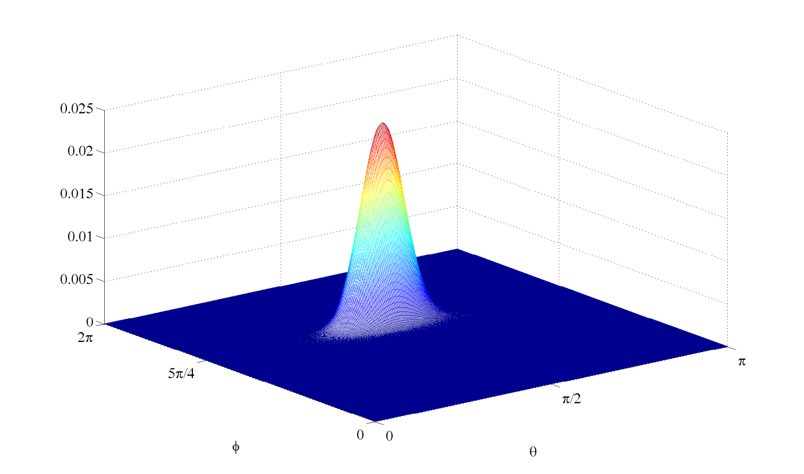
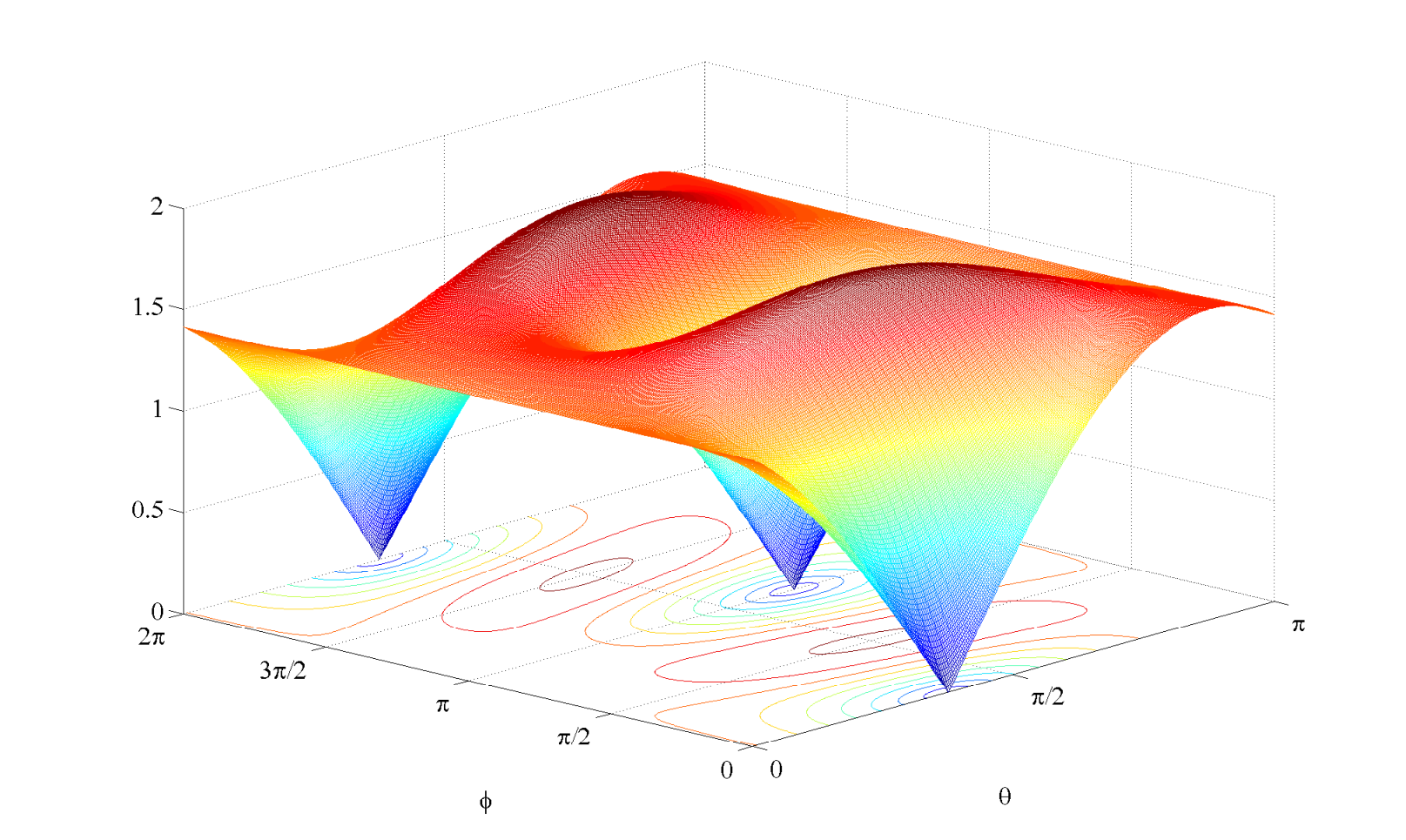
The norm of this object is peaked on configurations where the closure condition j1​n→1+j2​n→2+j3​n→3=0j_{1}\vec{n}_{1}+j_{2}\vec{n}_{2}+j_{3}\vec{n}_{3}=0 is satisfied, and the peak becomes sharper with increasing values of the spins j1j_{1}, j2j_{2} and j3j_{3}. This is a special case of the result obtained by Livine and Speziale [9] on the norm of the coherent intertwiner, since according to the discussion in section 2.3, the norm of (3.21) has an alternative interpretation as the norm of the three-valent coherent intertwiner |j1j2j3;n→1n→2n→3⟩|j_{1}j_{2}j_{3};\vec{n}_{1}\vec{n}_{2}\vec{n}_{3}\rangle. We nevertheless illustrate this property numerically in Figs. 1 and 2 below.

In Fig. 1, we plot the norm of (3.21) as a function of the polar angles of the vector n→3\vec{n}_{3}, when the first two vectors are fixed as n→1=(0,0,1)\vec{n}_{1}=(0,0,1) and n→2=(32,0,−12)\vec{n}_{2}=(\tfrac{\sqrt{3}}{2},0,-\tfrac{1}{2}), and the spins j1j_{1}, j2j_{2} and j3j_{3} are equal to a common value jj. We consider the values j=20j=20 and j=100j=100, and see that in both cases, the norm is peaked on n→3=−n→1−n→2\vec{n}_{3}=-\vec{n}_{1}-\vec{n}_{2}, corresponding to the angles (θ,ϕ)=(23​π,π)(\theta,\phi)=(\tfrac{2}{3}\pi,\pi), but the peak is sharper in the latter case. In Fig. 2, we show the norm of (3.21) when j1=j2=50j_{1}=j_{2}=50 and j3=86≈50​2j_{3}=86\approx 50\sqrt{2}, and we have fixed n→1=(1,0,0)\vec{n}_{1}=(1,0,0) and n→2=(0,1,0)\vec{n}_{2}=(0,1,0). The norm is peaked on the approximately closed configuration n→3=12​(−1,−1,0)\vec{n}_{3}=\tfrac{1}{\sqrt{2}}(-1,-1,0), corresponding to the angles (θ,ϕ)=(12​π,54​π)(\theta,\phi)=(\tfrac{1}{2}\pi,\tfrac{5}{4}\pi).

Refer to caption
Refer to caption
Figure 1: The norm of the 3jj-symbol (3.21) as a function of the polar angles of the vector n→3\vec{n}_{3}. The spins j1j_{1}, j2j_{2} and j3j_{3} are all equal to a common value jj, and the first two vectors are fixed to n→1=(0,0,1)\vec{n}_{1}=(0,0,1) and n→2=(32,0,−12)\vec{n}_{2}=(\tfrac{\sqrt{3}}{2},0,-\tfrac{1}{2}). In the upper diagram j=20j=20, and in the lower diagram j=100j=100. In both cases, the norm is peaked on the angles (θ,ϕ)=(23​π,π)(\theta,\phi)=(\tfrac{2}{3}\pi,\pi), corresponding to the closed configuration n→3=(−32,0,−12)=−n→1−n→2\vec{n}_{3}=(-\tfrac{\sqrt{3}}{2},0,-\tfrac{1}{2})=-\vec{n}_{1}-\vec{n}_{2}, but the peak is sharper when the spin jj is larger.
Refer to caption
Figure 2: The norm of (3.21) as a function of the polar angles of n→3\vec{n}_{3} when j1=j2=50j_{1}=j_{2}=50 and j3=86≈50​2j_{3}=86\approx 50\sqrt{2}. The maximum occurs at the angles (θ,ϕ)=(12​π,54​π)(\theta,\phi)=(\tfrac{1}{2}\pi,\tfrac{5}{4}\pi), corresponding to the vector n→3=(−12,−12,0)\vec{n}_{3}=(-\tfrac{1}{\sqrt{2}},{-\frac{1}{\sqrt{2}}},0). Therefore the norm is peaked on the approximately closed configuration n→1+n→2+2​n→3=0\vec{n}_{1}+\vec{n}_{2}+\sqrt{2}\vec{n}_{3}=0.

3.4 Raising and lowering indices in the coherent-state basis

Before concluding this section, we must discuss how indices of intertwiners are raised and lowered in the basis of coherent states. This is necessary for a consistent contraction of indices in an equation such as (2.38). In the basis of magnetic indices, indices are raised and lowered using the epsilon tensor; for example,

ιm1m2⋯mN=ϵ(j1)​m1​n1ιn1m2⋯mN.\iota\,^{m_{1}}_{\phantom{m_{1}}m_{2}\cdots m_{N}}=\epsilon^{(j_{1})m_{1}n_{1}}\iota_{n_{1}m_{2}\cdots m_{N}}. (3.22)

To derive the rule for raising an index in the coherent-state basis, we can compute the component of

∑m1⋯mNιm2⋯mNm1⟨j1m1|⊗|j2m2⟩⊗⋯⊗|jNmN⟩\sum_{m_{1}\cdots m_{N}}\iota\,^{m_{1}}_{\phantom{m_{1}}m_{2}\cdots m_{N}}\,\langle j_{1}m_{1}|\otimes|j_{2}m_{2}\rangle\otimes\cdots\otimes|j_{N}m_{N}\rangle (3.23)

with respect to the state ⟨j1ξ1|⊗|j2ξ2⟩⊗⋯⊗|jNξN⟩\langle j_{1}\xi_{1}|\otimes|j_{2}\xi_{2}\rangle\otimes\cdots\otimes|j_{N}\xi_{N}\rangle, or more directly consider the integral

ιξ2⋯ξNξ1=∫dμj1(η1)ϵ(j1)​ξ1​η1ιη1ξ2⋯ξN,\iota\,^{\xi_{1}}_{\phantom{\xi_{1}}\xi_{2}\cdots\xi_{N}}=\int d\mu_{j_{1}}(\eta_{1})\,\epsilon^{(j_{1})\xi_{1}\eta_{1}}\iota_{\eta_{1}\xi_{2}\cdots\xi_{N}}, (3.24)

which is Eq. (3.22) translated to the coherent-state basis. The coherent components of epsilon can be found, for example, by computing the projection of the state |ϵ⟩=∑m​nϵm​n(j)​|j​m⟩​|j​n⟩|\epsilon\rangle=\sum_{mn}\epsilon^{(j)}_{mn}|jm\rangle|jn\rangle onto the basis element |j​ξ⟩​|j​η⟩|j\xi\rangle|j\eta\rangle, or by noting that ϵm​n(j)=dj​(jj0mn0)\epsilon^{(j)}_{mn}=\sqrt{d_{j}}\bigl(\begin{smallmatrix}j&j&0\\ m&n&0\end{smallmatrix}\bigr) and using Eq. (3.9). One finds

ϵξ​η(j)=(ξ−η)2​j(1+|ξ|2)j​(1+|η|2)j\epsilon^{(j)}_{\xi\eta}=\frac{(\xi-\eta)^{2j}}{(1+|\xi|^{2})^{j}(1+|\eta|^{2})^{j}} (3.25)

and

ϵ(j)​ξ​η=ϵξ​η(j)¯.\epsilon^{(j)\xi\eta}=\overline{\epsilon^{(j)}_{\xi\eta}}. (3.26)

The integral (3.24) can then be evaluated using the integration formula (4.5), derived in the next section. The result is

ιξ1ξ2⋯ξN=ξ¯12​j1​Pι​(−ξ¯1−1,ξ2,…,ξN)(1+|ξ1|2)j1⋯(1+|ξN|2)jN.\iota\,^{\xi_{1}}_{\phantom{\xi_{1}}\xi_{2}\cdots\xi_{N}}=\frac{\bar{\xi}_{1}^{2j_{1}}P_{\iota}(-\bar{\xi}_{1}^{-1},\xi_{2},\dots,\xi_{N})}{(1+|\xi_{1}|^{2})^{j_{1}}\cdots(1+|\xi_{N}|^{2})^{j_{N}}}. (3.27)

This can alternatively be written as

ιξ1ξ2⋯ξN=Pι​(−ξ¯1−1,ξ2,…,ξN)(1+|−ξ¯1−1|2)j1⋯(1+|ξN|2)jN,\iota\,^{\xi_{1}}_{\phantom{\xi_{1}}\xi_{2}\cdots\xi_{N}}=\frac{P_{\iota}(-\bar{\xi}_{1}^{-1},\xi_{2},\dots,\xi_{N})}{(1+|{-}\bar{\xi}_{1}^{-1}|^{2})^{j_{1}}\cdots(1+|\xi_{N}|^{2})^{j_{N}}}, (3.28)

which shows that, when the intertwiner is described in terms of the vectors corresponding to the parameters ξ\xi, then raising an index ξa\xi_{a} is equivalent to replacing the corresponding vector n→a\vec{n}_{a} with −n→a-\vec{n}_{a}.

4 A polynomial representation of intertwiners

In the previous section we found that the components of an intertwiner with respect to the coherent state basis of ℋj1⊗⋯⊗ℋjN{\cal H}_{j_{1}}\otimes\cdots\otimes{\cal H}_{j_{N}}have the general form

ιξ1⋯ξN=Pι​(ξ1,…,ξN)(1+|ξ1|2)j1⋯(1+|ξN|2)jN.\iota_{\xi_{1}\cdots\xi_{N}}=\frac{P_{\iota}(\xi_{1},\dots,\xi_{N})}{(1+|\xi_{1}|^{2})^{j_{1}}\cdots(1+|\xi_{N}|^{2})^{j_{N}}}. (4.1)

In this section we will show that the polynomial Pι​(ξ1,…,ξN)P_{\iota}(\xi_{1},\dots,\xi_{N}) can itself be regarded as a representation of the intertwiner ι\iota. In section 4.1 we describe a representation of S​U​(2)SU(2) in the space 𝒫j{\cal P}_{j}, the space of polynomials of degree 2​j2j of a single complex variable. Then, in section 4.2 we show that the action of an angular momentum operator on the intertwiner ι\iota results in an action on the polynomial Pι​(ξ1,⋯,ξN)P_{\iota}(\xi_{1},\cdots,\xi_{N}) by a differential operator representing the angular momentum operator in the space 𝒫j{\cal P}_{j}. From this we conclude that Pι​(ξ1,⋯,ξN)P_{\iota}(\xi_{1},\cdots,\xi_{N}), regarded as an element of 𝒫j1⊗⋯⊗𝒫jN{\cal P}_{j_{1}}\otimes\cdots\otimes{\cal P}_{j_{N}}, is the representation of the intertwiner |ι⟩|\iota\rangle.

4.1 Representation of S​U​(2)SU(2) in a space of complex polynomials

A convenient realization of the spin-jj representation of S​U​(2)SU(2) can be constructed on the space of polynomials of degree 2​j2j in a complex variable zz (see e.g. [19]). We denote this space by 𝒫j{\cal P}_{j}; a general element of 𝒫j{\cal P}_{j} has the form f(j)​(z)=∑k=02​jck​zkf^{(j)}(z)=\sum_{k=0}^{2j}c_{k}z^{k}. A scalar product on 𝒫j{\cal P}_{j} can be defined as

⟨f(j)|g(j)⟩=∫d​νj​(z)​f(j)​(z)¯​g(j)​(z),\langle f^{(j)}|g^{(j)}\rangle=\int d\nu_{j}(z)\,\overline{f^{(j)}(z)}g^{(j)}(z), (4.2)

where the integration measure is

d​νj​(z)=djπ​d2​z(1+|z|2)2​j+2=d​μj​(z)(1+|z|2)2​jd\nu_{j}(z)=\frac{d_{j}}{\pi}\frac{d^{2}z}{(1+|z|^{2})^{2j+2}}=\frac{d\mu_{j}(z)}{(1+|z|^{2})^{2j}} (4.3)

with d​μj​(z)d\mu_{j}(z) the measure of Eq. (2.14). A basis of 𝒫j{\cal P}_{j}, orthonormal under the scalar product (4.2), is given by the monomials

fm(j)​(z)=(2​j)!(j+m)!​(j−m)!​zj+mf^{(j)}_{m}(z)=\sqrt{\frac{(2j)!}{(j+m)!(j-m)!}}z^{j+m} (4.4)

for m=−j,−j+1,…,jm=-j,-j+1,\dots,j. An immediate consequence of the orthonormality of the functions (4.4) is the useful identity

∫d​νj​(ξ)​(1+ξ¯​z)2​j​f(j)​(ξ)=f(j)​(z),\int d\nu_{j}(\xi)\,(1+\bar{\xi}z)^{2j}f^{(j)}(\xi)=f^{(j)}(z), (4.5)

valid for all functions f(j)∈𝒫jf^{(j)}\in{\cal P}_{j}.

A representation of S​U​(2)SU(2) on 𝒫j{\cal P}_{j} is obtained by defining the action of the group element gg of Eq. (A.1) on a function f(j)​(z)∈𝒫jf^{(j)}(z)\in{\cal P}_{j} to be

D(j)​(g)​f(j)​(z)=(β​z+α¯)2​j​f(j)​(α​z−β¯β​z+α¯).D^{(j)}(g)f^{(j)}(z)=(\beta z+\bar{\alpha})^{2j}f^{(j)}\biggl(\frac{\alpha z-\bar{\beta}}{\beta z+\bar{\alpha}}\biggr). (4.6)

In fact, this definition extends to the group S​L​(2,ℂ)SL(2,\mathbbm{C}); for h=(abcd)∈S​L​(2,ℂ)h=\bigl(\begin{smallmatrix}a&b\\ c&d\end{smallmatrix}\bigr)\in SL(2,\mathbbm{C}), the assignment

D(j)​(h)​f(j)​(z)=(b​z+d)2​j​f(j)​(a​z+cb​z+d)D^{(j)}(h)f^{(j)}(z)=(bz+d)^{2j}f^{(j)}\biggl(\frac{az+c}{bz+d}\biggr) (4.7)

defines a representation of S​L​(2,ℂ)SL(2,\mathbbm{C}) on 𝒫j{\cal P}_{j}.

To find the representation of the angular momentum operator on 𝒫j{\cal P}_{j}, we can use Eq. (4.7) and the explicit matrix representation of J→\vec{J} in the spin-1/2 representation (see Eq. (A.7)) to calculate, for example

eϵ​J+​f(j)​(z)=(1+ϵ​z)2​j​f(j)​(z1+ϵ​z).e^{\epsilon J_{+}}f^{(j)}(z)=(1+\epsilon z)^{2j}f^{(j)}\biggl(\frac{z}{1+\epsilon z}\biggr). (4.8)

Expanding both sides to first order in ϵ\epsilon then reveals that

J+=−z2​dd​z+2​j​z.J_{+}=-z^{2}\frac{d}{dz}+2jz. (4.9)

By similar calculations one finds

J0=z​dd​z−jJ_{0}=z\frac{d}{dz}-j (4.10)

and

J−=dd​z.J_{-}=\frac{d}{dz}. (4.11)

It is immediate to check that the function fm(j)f^{(j)}_{m} of Eq. (4.4) is an eigenstate of J0J_{0} with eigenvalue mm, and hence corresponds to the state |j​m⟩∈ℋj|jm\rangle\in{\cal H}_{j} in standard physics notation.

For reference, let us write down the angular momentum coherent state |jξ⟩=D(j)(ξ)|j,−j⟩|j\xi\rangle=D^{(j)}(\xi)|j,-{}j\rangle as an element of 𝒫j{\cal P}_{j}. Using Eqs. (2.12) and (4.7), and noting that the state |j,−j⟩|j,-{}j\rangle corresponds to the element f−j(j)​(z)=1f^{(j)}_{-j}(z)=1 of 𝒫j{\cal P}_{j}, we find

fξ(j)​(z)=1(1+|ξ|2)j​(1+ξ¯​z)2​j.f_{\xi}^{(j)}(z)=\frac{1}{(1+|\xi|^{2})^{j}}(1+\bar{\xi}z)^{2j}. (4.12)

The polynomial representing the unnormalized coherent state |jξ)|j\xi) of Eq. (2.18) is simply (1+ξ¯​z)2​j(1+\bar{\xi}z)^{2j}. In this notation, the integration formula (4.5) is expressed as

∫d​νj​(ξ)​(j​ξ|j​z)​f(j)​(ξ)=f(j)​(z).\int d\nu_{j}(\xi)\,(j\xi|jz)f^{(j)}(\xi)=f^{(j)}(z). (4.13)

Let us also note that the matrix elements of the angular momentum operator between the states |jξ)|j\xi), computed in section 2.2, can now be written as

(j​ξ​|Jμ|​j​η)=Jμ​(ξ¯)​(j​ξ|j​η),(j\xi|J_{\mu}|j\eta)=J_{\mu}(\bar{\xi})(j\xi|j\eta), (4.14)

where Jμ​(ξ¯)J_{\mu}(\bar{\xi}) (μ=+,0,−)(\mu=+,0,-) denotes any of the differential operators of Eqs. (4.9)–(4.11) acting on the variable ξ¯\bar{\xi}.

4.2 Intertwiners as elements of 𝒫j{\cal P}_{j}

We will now show how a polynomial representation of the intertwiner |ι⟩|\iota\rangle can be extracted from the explicit expression of ιξ1⋯ξN\iota_{\xi_{1}\cdots\xi_{N}}. The component of the intertwiner |ι⟩|\iota\rangle with respect to the basis state |j1ξ1⊗⋯⊗jNξN⟩|j_{1}\xi_{1}\otimes\cdots\otimes j_{N}\xi_{N}\rangle is given by the complex conjugate of the object ιξ1⋯ξN\iota_{\xi_{1}\cdots\xi_{N}} of Eq. (3.18). Therefore, |ι⟩|\iota\rangle can be expanded in the basis of coherent states as

|ι⟩=∫dμj1(ξ1)⋯dμjN(ξN)ιξ1⋯ξN¯|j1ξ1⊗⋯⊗jNξN⟩.|\iota\rangle=\int d\mu_{j_{1}}(\xi_{1})\cdots d\mu_{j_{N}}(\xi_{N})\,\overline{\iota_{\xi_{1}\cdots\xi_{N}}}\,|j_{1}\xi_{1}\otimes\cdots\otimes j_{N}\xi_{N}\rangle. (4.15)

For the sake of clarity, let us first consider the action of a single angular momentum operator, acting on the first spin of the state |ι⟩|\iota\rangle. Projecting the resulting state on the basis element ⟨j1η1⊗⋯⊗jNηN|\langle j_{1}\eta_{1}\otimes\cdots\otimes j_{N}\eta_{N}|, inserting the form of ιξ1⋯ξN\iota_{\xi_{1}\cdots\xi_{N}} given by Eq. (3.18), and introducing the unnormalized states |jξ)|j\xi) from Eq. (2.18) and the measure d​νj​(ξ)d\nu_{j}(\xi) from Eq. (4.3), we obtain

⟨j1η1⊗⋯⊗jNηN|Jμ(1)|ι⟩=1(1+|η1|2)j1⋯(1+|ηN|2)jN\displaystyle\langle j_{1}\eta_{1}\otimes\cdots\otimes j_{N}\eta_{N}|J_{\mu}^{(1)}|\iota\rangle=\frac{1}{(1+|\eta_{1}|^{2})^{j_{1}}\cdots(1+|\eta_{N}|^{2})^{j_{N}}}
×∫dνj1(ξ1)⋯dνjN(ξN)Pι(ξ¯1,…,ξ¯N)(j1η1|Jμ|j1ξ1)(j2η2|j2ξ2)⋯(jNηN|jNξN).\displaystyle{}\times\int d\nu_{j_{1}}(\xi_{1})\,\cdots d\nu_{j_{N}}(\xi_{N})\,P_{\iota}(\bar{\xi}_{1},\dots,\bar{\xi}_{N})\,(j_{1}\eta_{1}|J_{\mu}|j_{1}\xi_{1})(j_{2}\eta_{2}|j_{2}\xi_{2})\cdots(j_{N}\eta_{N}|j_{N}\xi_{N}). (4.16)

To perform the integral, we first recall that (j1​η1​|Jμ(1)|​j1​ξ1)=Jμ​(η¯1)​(j1​η1|j1​ξ1)(j_{1}\eta_{1}|J_{\mu}^{(1)}|j_{1}\xi_{1})=J_{\mu}(\bar{\eta}_{1})(j_{1}\eta_{1}|j_{1}\xi_{1}), and then write (j​η|j​ξ)=(j​ξ¯|j​η¯)(j\eta|j\xi)=(j\bar{\xi}|j\bar{\eta}). This allows us to evaluate the integral using Eq. (4.13); the result is Jμ​(η¯1)​P​(η¯1,⋯,η¯N)J_{\mu}(\bar{\eta}_{1})P(\bar{\eta}_{1},\cdots,\bar{\eta}_{N}). We therefore conclude

⟨j1η1⊗⋯⊗jNηN|Jμ(1)|ι⟩=Jμ​(η¯1)​Pι​(η¯1,…,η¯N)(1+|η1|2)j1⋯(1+|ηN|2)jN.\langle j_{1}\eta_{1}\otimes\cdots\otimes j_{N}\eta_{N}|J_{\mu}^{(1)}|\iota\rangle=\frac{J_{\mu}(\bar{\eta}_{1})P_{\iota}(\bar{\eta}_{1},\dots,\bar{\eta}_{N})}{(1+|\eta_{1}|^{2})^{j_{1}}\cdots(1+|\eta_{N}|^{2})^{j_{N}}}. (4.17)

By a similar calculation we can show that for any operator 𝒪⁡(J(1),⋯,J(N)){\cal O}(J^{(1)},\cdots,J^{(N)}), constructed from the angular momentum operators by a power series expansion, we have55 5 As indicated by Eq. (4.15), we consider an intertwiner whose all indices are lower indices. For each upper index of the intertwiner, the corresponding angular momentum operator Jm(a)J^{(a)}_{m} should be replaced with (J(a)​μ)†=J−μ(a)(J^{(a)}\mu)^{\dagger}=J^{(a)}_{-\mu} in 𝒪⁡(J(1),⋯,J(N)){\cal O}(J^{(1)},\cdots,J^{(N)}) in Eq. (4.18).

⟨j1ξ1⊗⋯⊗jNξN|𝒪(J(1),⋯,J(N))|ι⟩=𝒪⁡(J⁡(ξ¯1),⋯,J⁡(ξ¯N))​Pι​(ξ¯1,…,ξ¯N)(1+|ξ1|2)j1⋯(1+|ξN|2)jN.\langle j_{1}\xi_{1}\otimes\cdots\otimes j_{N}\xi_{N}|{\cal O}(J^{(1)},\cdots,J^{(N)})|\iota\rangle=\frac{{\cal O}\bigl(J(\bar{\xi}_{1}),\cdots,J(\bar{\xi}_{N})\bigr)P_{\iota}(\bar{\xi}_{1},\dots,\bar{\xi}_{N})}{(1+|\xi_{1}|^{2})^{j_{1}}\cdots(1+|\xi_{N}|^{2})^{j_{N}}}. (4.18)

That is, the action of the angular momentum operator on the state |ι⟩|\iota\rangle translates to an action on the polynomial Pι​(ξ1,…,ξN)P_{\iota}(\xi_{1},\dots,\xi_{N}) by the differential-operator representation of the angular momentum operator on the space 𝒫j1⊗⋯⊗𝒫jN{\cal P}_{j_{1}}\otimes\cdots\otimes{\cal P}_{j_{N}}. This confirms that we can consistently interpret Pι​(ξ1,…,ξN)P_{\iota}(\xi_{1},\dots,\xi_{N}) as the element of 𝒫j1⊗⋯⊗𝒫jN{\cal P}_{j_{1}}\otimes\cdots\otimes{\cal P}_{j_{N}} corresponding to the intertwiner |ι⟩|\iota\rangle. In this description of the intertwiner, the variable ξa\xi_{a} is no longer regarded as a parameter specifying an unit vector n→a\vec{n}_{a}, but only as an abstract variable, whose first 2​ja2j_{a} powers span the space 𝒫ja{\cal P}_{j_{a}}.

5 Application to calculations in LQG

As a concerete example of applying the techniques developed in the previous sections to calculations in loop quantum gravity, let us consider the operator

Ca​b=ϵi​j​k​Tr(l)​(τk​hαa​b)​Ji(a)​Jj(b),C_{ab}=\epsilon_{ijk}\,{\rm Tr}^{(l)}\bigl(\tau_{k}h_{\alpha_{ab}}\bigr)J^{(a)}_{i}J^{(b)}_{j}, (5.1)

which is used to construct the physical Hamiltonian in a model of loop quantum gravity deparametrized with respect to a free scalar field. (For more details, see [4].) The operator Ca​bC_{ab} acts on a pair of edges eae_{a} and ebe_{b} sharing a node in a spin network state, the two angular momentum operators Ji(a)J^{(a)}_{i} and Jj(b)J^{(b)}_{j} acting on the holonomies associated with the two edges. Furthermore, hαa​bh_{\alpha_{ab}} denotes a holonomy around a loop αa​b\alpha_{ab}, which is attached to the graph of the spin network and is tangent to, but does not overlap with, the two edges eae_{a} and ebe_{b}. Finally, τk=−iσk/2\tau_{k}=-i\sigma_{k}/2 denotes the anti-Hermitian generators of S​U​(2)SU(2).

Therefore, at the level of intertwiners described in the standard basis of magnetic indices, the action of the operator Ca​bC_{ab} is to replace the original intertwiner ιm1⋯mN\iota_{m_{1}\cdots m_{N}} at the node with a new intertwiner (Ca​bι)m1⋯mNn1n2(C_{ab}\iota)_{m_{1}\cdots m_{N}n_{1}n_{2}}. The two new indices of the new intertwiner are in the end contracted with the representation matrix Dn1​n2(l)​(hαa​b)D^{(l)}_{n_{1}n_{2}}(h_{\alpha_{ab}}) of the holonomy around the loop αa​b\alpha_{ab}.

The action of the operator Ca​bC_{ab} on an intertwiner in the coherent-state basis can be found by evaluating the object

(Ca​bι)ξ1⋯ξNη1η2≡⟨ϵi​j​k(τk(l))η1​η2Ji(a)Jj(b)ι|j1ξ1⊗⋯⊗jNξN⟩,(C_{ab}\iota)_{\xi_{1}\cdots\xi_{N}\eta_{1}\eta_{2}}\equiv\langle\epsilon_{ijk}(\tau_{k}^{(l)})_{\eta_{1}\eta_{2}}J^{(a)}_{i}J^{(b)}_{j}\,\iota|j_{1}\xi_{1}\otimes\cdots\otimes j_{N}\xi_{N}\rangle, (5.2)

where the indices η1\eta_{1} and η2\eta_{2} are eventually contracted with the indices of the representation matrix Dη1​η2(l)​(hαa​b)D^{(l)}_{\eta_{1}\eta_{2}}(h_{\alpha_{ab}}) by the integral ∫d​μl​(η1)​d​μl​(η2)\int d\mu_{l}(\eta_{1})\,d\mu_{l}(\eta_{2}). On grounds of Eq. (4.18), we obtain from Eq. (5.2)

(Ca​bι)ξ1⋯ξNη1η2=(Ca​b​Pι)​(ξ1,⋯,ξN,η1,η2)(1+|ξ1|2)j1⋯(1+|ξN|2)jN(1+|η1|2)l(1+|η2|2)l,(C_{ab}\iota)_{\xi_{1}\cdots\xi_{N}\eta_{1}\eta_{2}}=\frac{(C_{ab}P_{\iota})(\xi_{1},\cdots,\xi_{N},\eta_{1},\eta_{2})}{(1+|\xi_{1}|^{2})^{j_{1}}\cdots(1+|\xi_{N}|^{2})^{j_{N}}(1+|\eta_{1}|^{2})^{l}(1+|\eta_{2}|^{2})^{l}}, (5.3)

where (Ca​b​Pι)​(ξ1,⋯,ξN,η1,η2)(C_{ab}P_{\iota})(\xi_{1},\cdots,\xi_{N},\eta_{1},\eta_{2}) is a polynomial which represents the new intertwiner as an element of 𝒫j1⊗⋯⊗𝒫jN⊗𝒫l⊗𝒫l{\cal P}_{j_{1}}\otimes\cdots\otimes{\cal P}_{j_{N}}\otimes{{\cal P}_{l}}\otimes{\cal P}_{l}. An expression for Ca​b​PιC_{ab}P_{\iota} can be derived by using Eqs. (4.9)–(4.11) for the angular momentum operators, and the explicit form of the matrix elements (τk(l))η1​η2=−i2​⟨l​η1|Jk|l​η2⟩(\tau_{k}^{(l)})_{\eta_{1}\eta_{2}}=-\tfrac{i}{2}\langle l\eta_{1}|J_{k}|l\eta_{2}\rangle given by Eqs. (2.25)–(2.27). Introducing the abbreviations ∂a=∂/∂ξa\partial_{a}=\partial/\partial\xi_{a} and ∂2a​b=∂2/∂ξa∂ξb\partial^{2}_{ab}=\partial^{2}/\partial\xi_{a}\partial\xi_{b}, we find

(Ca​bPι)(ξ1,⋯,ξN,η1,η2)=l2(1+η1η¯2)2​l−1[η1((ξa−ξb)∂a​b2+jb∂a−ja∂b)\displaystyle(C_{ab}P_{\iota})(\xi_{1},\cdots,\xi_{N},\eta_{1},\eta_{2})=\frac{l}{2}(1+\eta_{1}\bar{\eta}_{2})^{2l-1}\biggl[\eta_{1}\Bigl((\xi_{a}-\xi_{b})\partial^{2}_{ab}+j_{b}\partial_{a}-j_{a}\partial_{b}\Bigr)
+η¯2(−ξaξb(ξa−ξb)∂a​b2+jbξa(ξa−2ξb)∂a−jaξb(ξb−2ξa)∂b−2jajb(ξa−ξb))\displaystyle+\bar{\eta}_{2}\Bigl(-\xi_{a}\xi_{b}(\xi_{a}-\xi_{b})\partial^{2}_{ab}+j_{b}\xi_{a}(\xi_{a}-2\xi_{b})\partial_{a}-j_{a}\xi_{b}(\xi_{b}-2\xi_{a})\partial_{b}-2j_{a}j_{b}(\xi_{a}-\xi_{b})\Bigr)
+(η1η¯2−1)(12(ξa2−ξb2)∂a​b2+jbξb∂a−jaξa∂b)]Pι(ξ1,…,ξN).\displaystyle+(\eta_{1}\bar{\eta}_{2}-1)\Bigl(\tfrac{1}{2}(\xi_{a}^{2}-\xi_{b}^{2})\partial^{2}_{ab}+j_{b}\xi_{b}\partial_{a}-j_{a}\xi_{a}\partial_{b}\Bigr)\biggr]P_{\iota}(\xi_{1},\dots,\xi_{N}). (5.4)

On a general level, we cannot make Eqs. (5.3) and (5.4) more explicit, since we lack a general expression for the polynomial Pι​(ξ1,…,ξN)P_{\iota}(\xi_{1},\dots,\xi_{N}). Let us therefore specialize to the case of computing the action of the operator C12C_{12} on a three-valent intertwiner. In this case, the explicit form of Pι​(ξ1,ξ2,ξ3)P_{\iota}(\xi_{1},\xi_{2},\xi_{3}) can be read off from Eq. (3.9) as

Pι​(ξ1,ξ2,ξ3)=(ξ1−ξ2)j1+j2−j3​(ξ2−ξ3)j2+j3−j1​(ξ3−ξ1)j3+j1−j2.P_{\iota}(\xi_{1},\xi_{2},\xi_{3})=(\xi_{1}-\xi_{2})^{j_{1}+j_{2}-j_{3}}(\xi_{2}-\xi_{3})^{j_{2}+j_{3}-j_{1}}(\xi_{3}-\xi_{1})^{j_{3}+j_{1}-j_{2}}. (5.5)

Introducing the notation ξa​b=ξa−ξb\xi_{ab}=\xi_{a}-\xi_{b} and ka=j1+j2+j3−2​jak_{a}=j_{1}+j_{2}+j_{3}-2j_{a}, it is convenient to write the derivatives appearing in Eq. (5.4) as

∂1Pι​(ξ1,ξ2,ξ3)\displaystyle\partial_{1}P_{\iota}(\xi_{1},\xi_{2},\xi_{3}) =(k3ξ12−k2ξ31)​Pι​(ξ1,ξ2,ξ3),\displaystyle=\biggl(\frac{k_{3}}{\xi_{12}}-\frac{k_{2}}{\xi_{31}}\biggr)P_{\iota}(\xi_{1},\xi_{2},\xi_{3}), (5.6)
∂2Pι​(ξ1,ξ2,ξ3)\displaystyle\partial_{2}P_{\iota}(\xi_{1},\xi_{2},\xi_{3}) =(k1ξ23−k3ξ12)​Pι​(ξ1,ξ2,ξ3)\displaystyle=\biggl(\frac{k_{1}}{\xi_{23}}-\frac{k_{3}}{\xi_{12}}\biggr)P_{\iota}(\xi_{1},\xi_{2},\xi_{3}) (5.7)

and

∂12Pι​(ξ1,ξ2,ξ3)=(−k32−k2ξ122−k1​k2ξ23​ξ31+k2k3​ξ31​ξ12+k3​k1ξ12​ξ23)​Pι​(ξ1,ξ2,ξ3).\partial_{12}P_{\iota}(\xi_{1},\xi_{2},\xi_{3})=\biggl(-\frac{k_{3}^{2}-k^{2}}{\xi_{12}^{2}}-\frac{k_{1}k_{2}}{\xi_{23}\xi_{31}}+\frac{k_{2}}{k_{3}}{\xi_{31}\xi_{12}}+\frac{k_{3}k_{1}}{\xi_{12}\xi_{23}}\biggr)P_{\iota}(\xi_{1},\xi_{2},\xi_{3}). (5.8)

This suggests to express the components of the intertwiner C12​ιC_{12}\iota, given by Eq. (5.3), by factoring out the component of the original intertwiner, (j1j2j3ξ1ξ2ξ3)\bigl(\begin{smallmatrix}j_{1}&j_{2}&j_{3}\\ \xi_{1}&\xi_{2}&\xi_{3}\end{smallmatrix}\bigr). We can also separate the factor (1+η1​η¯2)2​l/(1+|η1|2)l​(1+|η2|2)l=⟨l​η2|l​η1⟩(1+\eta_{1}\bar{\eta}_{2})^{2l}/(1+|\eta_{1}|^{2})^{l}(1+|\eta_{2}|^{2})^{l}=\langle l\eta_{2}|l\eta_{1}\rangle, which, up to a phase, is equal to [12​(1+n→η1⋅n→η2)]l[\tfrac{1}{2}(1+\vec{n}_{\eta_{1}}\cdot\vec{n}_{\eta_{2}})]^{l}. In this way, we can write the components of the new intertwiner in the form

(Ca​b​ι)ξ1​ξ2​ξ3​η1​η2=F⁡(ξ1,ξ2,ξ3,η1,η2)​(1+n→η1⋅n→η22)l​(j1j2j3ξ1ξ2ξ3),(C_{ab}\iota)_{\xi_{1}\xi_{2}\xi_{3}\eta_{1}\eta_{2}}=F(\xi_{1},\xi_{2},\xi_{3},\eta_{1},\eta_{2})\biggl(\frac{1+\vec{n}_{\eta_{1}}\cdot\vec{n}_{\eta_{2}}}{2}\biggr)^{l}\begin{pmatrix}j_{1}&j_{2}&j_{3}\\ \xi_{1}&\xi_{2}&\xi_{3}\end{pmatrix}, (5.9)

where n→ηa\vec{n}_{\eta_{a}} denotes the vector corresponding to the parameter ηa\eta_{a}, and F⁡(ξ1,ξ2,ξ3,η1,η2)F(\xi_{1},\xi_{2},\xi_{3},\eta_{1},\eta_{2}) is a function which can be determined using Eqs. (5.4) and (5.6)–(5.8).

In the limit of large spins, the expression (5.9) admits the following interpretation in terms of the vectors corresponding to the parameters ξa\xi_{a} and ηa\eta_{a}. As discussed in section 3.3, in the large-jj limit the 3jj-symbol in Eq. (5.9) is suppressed unless the vectors n→a\vec{n}_{a} corresponding to the parameters ξa\xi_{a} satisfy the closure condition j1​n→1+j2​n→2+j3​n→3=0j_{1}\vec{n}_{1}+j_{2}\vec{n}_{2}+j_{3}\vec{n}_{3}=0. Similarly, the factor [12​(1+n→η1⋅n→η2)]l[\tfrac{1}{2}(1+\vec{n}_{\eta_{1}}\cdot\vec{n}_{\eta_{2}})]^{l} forces the two vectors n→η1\vec{n}_{\eta_{1}} and n→η2\vec{n}_{\eta_{2}} to be parallel to each other, when the value of ll is large. Assuming that the vectors ja​n→aj_{a}\vec{n}_{a} close, and that n→η1=n→η2≡n→η\vec{n}_{\eta_{1}}=\vec{n}_{\eta_{2}}\equiv\vec{n}_{\eta}, we can look at the function FF to determine the preferred orientation of the vector n→η\vec{n}_{\eta} relative to the vectors n→a\vec{n}_{a}.

As a first example, let us examine the case where the spins j1j_{1}, j2j_{2} and j3j_{3} are equal to a common value jj. If we fix n→1=12​(3,0,−1)\vec{n}_{1}=\tfrac{1}{2}(\sqrt{3},0,-1), n→2=12​(−3,0,−1)\vec{n}_{2}=\tfrac{1}{2}(-\sqrt{3},0,-1) and n→3=(0,0,1)\vec{n}_{3}=(0,0,1), we find that the absolute value of the function FF is given in terms of the polar angles of the vector n→η\vec{n}_{\eta} as

|F(θη,ϕη)|=3j2l(|sinθηsinϕη|+𝒪(j−1)).|F(\theta_{\eta},\phi_{\eta})|=\sqrt{3}j^{2}l\Bigl(|\sin\theta_{\eta}\sin\phi_{\eta}|+{\cal O}(j^{-1})\Bigr). (5.10)

This function is evidently maximized when θη=π/2\theta_{\eta}=\pi/2, and ϕη=π/2\phi_{\eta}=\pi/2 or ϕη=3​π/2\phi_{\eta}=3\pi/2, i.e. when n→η=(0,±1,0)\vec{n}_{\eta}=(0,{\pm}1,0). In other words, the preferred orientation of the vector n→η\vec{n}_{\eta} is orthogonal to the plane spanned by the vectors n→1\vec{n}_{1}, n→2\vec{n}_{2} and n→3\vec{n}_{3}. This conclusion is independent of the values of the spins jj and ll, since up to subleading terms the absolute value |F⁡(θη,ϕη)||F(\theta_{\eta},\phi_{\eta})| depends on jj and ll only through an overall multiplicative factor.

As another example we give the case j1=j2=jj_{1}=j_{2}=j and j3≈2​jj_{3}\approx\sqrt{2}j. To satisfy the closure condition of the vectors n→a\vec{n}_{a}, we now fix n→1=(0,0,1)\vec{n}_{1}=(0,0,1), n→2=(1,0,0)\vec{n}_{2}=(1,0,0) and n→3=12​(−1,0,−1)\vec{n}_{3}=\tfrac{1}{\sqrt{2}}(-1,0,-1). Now the explicit expression of |F⁡(θη,ϕη)||F(\theta_{\eta},\phi_{\eta})| is unenlightening, so we show a numerical plot of |F⁡(θη,ϕη)|/j2​l|F(\theta_{\eta},\phi_{\eta})|/j^{2}l (which is independent of j2j^{2} and ll at leading order) in Fig. 3 below. The plot indicates that the preferred orientation of the vectors n→η\vec{n}_{\eta} is still perpendicular to the plane of the vectors n→1\vec{n}_{1}, n→2\vec{n}_{2} and n→3\vec{n}_{3}.

Refer to caption
Figure 3: A plot of the function |F⁡(θη,ϕη)|/j2​l|F(\theta_{\eta},\phi_{\eta})|/j^{2}l, when the spins of the three-valent intertwiner ι\iota are given by j1=j2=jj_{1}=j_{2}=j and j3≈2​jj_{3}\approx\sqrt{2}j. The function F⁡(θη,ϕη)F(\theta_{\eta},\phi_{\eta}) determines the preferred orientation of the vectors n→η1=n→η2≡n→η\vec{n}_{\eta_{1}}=\vec{n}_{\eta_{2}}\equiv\vec{n}_{\eta}, created by the action of the operator C12C_{12} on the intertwiner ι\iota. The maxima of the function |F⁡(θη,ϕη)||F(\theta_{\eta},\phi_{\eta})| are located at (θη,ϕη)=(12​π,12​π)(\theta_{\eta},\phi_{\eta})=(\tfrac{1}{2}\pi,\tfrac{1}{2}\pi) and (θη,ϕη)=(12​π,32​π)(\theta_{\eta},\phi_{\eta})=(\tfrac{1}{2}\pi,\tfrac{3}{2}\pi). Both points correspond to the vector n→η\vec{n}_{\eta} orthogonal to the plane of the vectors n→1\vec{n}_{1}, n→2\vec{n}_{2} and n→3\vec{n}_{3}.

6 Conclusions

In this work we studied intertwiners projected onto the basis of angular momentum coherent states. The relevance of our calculations to loop quantum gravity is twofold. Firstly, the object ιξ1⋯ξN\iota_{\xi_{1}\cdots\xi_{N}}, defined in Eq. (3.1) and given in explicit form in Eqs. (3.9) and (3.16) in the case of three- and four-valent intertwiners, provides an expression for the components of the Livine–Speziale coherent intertwiner |j1⋯jN;ξ1⋯ξN⟩|j_{1}\cdots j_{N};\xi_{1}\cdots\xi_{N}\rangle with respect to the standard basis {|ι⟩}\{|\iota\rangle\} of the intertwiner space. Secondly, and more importantly, by rewriting the spin network states of loop quantum gravity in terms of intertwiners projected on coherent states, operators such as the Hamiltonian can be reformulated as differential operators acting on polynomials of the complex variables ξa\xi_{a}.

The primary motivation for our work is to introduce an alternative approach towards analyzing the matrix elements of the Hamiltonian operator, in which the use of S​U​(2)SU(2) recoupling theory is bypassed. By rewriting the spin network states and the Hamiltonian in the language of the complex numbers ξa\xi_{a}, and by providing explicit expressions for the projections of intertwiners on coherent states, we make it possible to describe the action of the Hamiltonian geometrically, in terms of the vectors corresponding to the parameters ξa\xi_{a}. This was illustrated by the example in section 5, where we considered (the Euclidean part of) the physical Hamiltonian of a deparametrized model of loop quantum gravity [4]. We computed the action of the operator on a three-valent intertwiner, and found that the preferred orientation of the two new vectors created by the Hamiltonian is orthogonal to the plane containing the three vectors of the original intertwiner.

Our expectation is that the techniques presented in this work will be useful for gaining a more controlled analytical understanding of the Hamiltonian in loop quantum gravity, and eventually for studying the semiclassical limit of the dynamics through an asymptotic analysis of the matrix elements of the Hamiltonian (e.g. via saddle point techniques). However, the scope of the present paper is merely to show that the coherent states of angular momentum can be used to develop an alternative framework for performing calculations with the Hamiltonian. Carrying out a systematic analysis of the dynamics and obtaining a clear understanding of the geometrical content of the Hamiltonian in this framework is a question left for future work.

Acknowledgments

The work of EA and JL was supported by the grant of Polish Narodowe Centrum Nauki nr DEC-2011/02/A/ST2/00300. EA wishes to acknowledge the John Templeton Foundation for the supporting grant #51876. IM would like to thank the Jenny and Antti Wihuri Foundation for support.

Appendix A Selected facts about S​U​(2)SU(2)

In this appendix we recall some results from S​U​(2)SU(2) representation theory, which will be needed in the main text.

A.1 Parametrizations of S​U​(2)SU(2)

A general element g∈S​U​(2)g\in SU(2) has the form

g=(αβ−β¯α¯)where|α|2+|β|2=1.g=\begin{pmatrix}\alpha&\beta\\ -\bar{\beta}&\bar{\alpha}\end{pmatrix}\qquad\text{where}\quad|\alpha|^{2}+|\beta|^{2}=1. (A.1)

The group element can be parametrized in terms of an angle χ\chi and an axis of rotation n→\vec{n} as

g=e−iχn→⋅J→=cosχ2−isinχ2(n→⋅σ→),g=e^{-i\chi\vec{n}\cdot\vec{J}}=\cos\frac{\chi}{2}-i\sin\frac{\chi}{2}(\vec{n}\cdot\vec{\sigma}), (A.2)

where J→=σ→/2\vec{J}=\vec{\sigma}/2 is the angular momentum operator for j=1/2j=1/2, and σ→=(σx,σy,σz)\vec{\sigma}=(\sigma_{x},\sigma_{y},\sigma_{z}) are the Pauli matrices.

Further parametrizations of the group element can be obtained using the operators J±=Jx±i​JyJ_{\pm}=J_{x}\pm iJ_{y} and J0=JzJ_{0}=J_{z}. One has the decompositions

g=eλ​J−​eμ​J0​eν​J+g=e^{\lambda J_{-}}e^{\mu J_{0}}e^{\nu J_{+}} (A.3)

and

g=eξ​J+​eη​J0​eζ​J−g=e^{\xi J_{+}}e^{\eta J_{0}}e^{\zeta J_{-}} (A.4)

where the parameters are given by

eμ/2=αλ=−β¯αν=βαe^{\mu/2}=\alpha\qquad\lambda=-\frac{\bar{\beta}}{\alpha}\qquad\nu=\frac{\beta}{\alpha} (A.5)

and

e−η/2=α¯ξ=βα¯ζ=−β¯α¯.e^{-\eta/2}=\bar{\alpha}\qquad\xi=\frac{\beta}{\bar{\alpha}}\qquad\zeta=-\frac{\bar{\beta}}{\bar{\alpha}}. (A.6)

The relations (A.3) and (A.4) can be verified by direct calculation in the fundamental representation of the group, using an explicit matrix representation for the angular momentum operators66 6 The standard representation of J→\vec{J} is given in the basis in which JzJ_{z} is diagonal, and reads Jx=12​(0110),Jy=12​(0−ii0),Jz=12​(100−1).J_{x}=\frac{1}{2}\begin{pmatrix}0&1\\ 1&0\end{pmatrix},\qquad J_{y}=\frac{1}{2}\begin{pmatrix}0&-i\\ i&0\end{pmatrix},\qquad J_{z}=\frac{1}{2}\begin{pmatrix}1&0\\ 0&-1\end{pmatrix}. (A.7) . Note that in general, none of the matrices on the right-hand side of Eqs. (A.3) and (A.4) are elements of S​U​(2)SU(2), though they do belong S​L​(2,ℂ)SL(2,\mathbbm{C}).

A.2 The spin-jj representation as a symmetric tensor product

The fundamental (spin-1/2) representation of S​U​(2)SU(2) is realized by letting the matrix g=gBAg=g^{A}_{\;\;B} of Eq. (A.1) act on the space ℋ1/2≅ℂ2{\cal H}_{1/2}\cong\mathbbm{C}^{2} spanned by the vectors vAv^{A}, the index AA taking the two values A=+,−A=+,-. A realization of the spin-jj representation that is sometimes useful is obtained by considering the space ℋj{\cal H}_{j} as the completely symmetric part of the tensor product of 2​j2j copies of the space ℋ1/2{\cal H}_{1/2}. Hence, ℋj{\cal H}_{j} is spanned by the dj=2​j+1d_{j}=2j+1 vectors v(A1⋯A2​j)≡vmv^{(A_{1}\cdots A_{2j})}\equiv v^{m}; the correspondence between the completely symmetric index (A1⋯A2​j)(A_{1}\cdots A_{2j}) and the magnetic index mm typically used in the physics literature is given by m=12​∑i=12​jAim=\tfrac{1}{2}\sum_{i=1}^{2j}A_{i}. The representation of an element g∈S​U​(2)g\in SU(2) on the space ℋ{\cal H} is then given by

Dm​n(j)(g)=D(A1⋯A2​j)(B1⋯B2​j)(j)(g)=g(B1CLOSEA1⋯gOPENB2​j)A2​j.D^{(j)}_{mn}(g)=D^{(j)}_{(A_{1}\cdots A_{2j})(B_{1}\cdots B_{2j})}(g)=g^{A_{1}}_{\hskip 8.19447pt(B_{1}}\cdots g^{A_{2j}}_{\hskip 8.19447ptB_{2j})}. (A.8)

Intertwiners – i.e. invariant tensors on ℋj1⊗⋯⊗ℋjN{\cal H}_{j_{1}}\otimes\cdots\otimes{\cal H}_{j_{N}} – are constructed using the tensor ϵA​B\epsilon_{AB}, which is the only invariant tensor in the fundamental representation77 7 Together with δBA\delta^{A}_{B} and ϵA​B\epsilon^{AB}, which are obtained by raising one or both indices of ϵA​B\epsilon_{AB}. Indices are raised and lowered according to the conventions vA=ϵA​B​vB,vA=vB​ϵB​A.v^{A}=\epsilon^{AB}v_{B},\qquad v_{A}=v^{B}\epsilon_{BA}. (A.9) . For example, the three-valent intertwiner between representations j1j_{1}, j2j_{2} and j3j_{3} is given by

ιm1​m2​m3(j1​j2​j3)\displaystyle\iota^{(j_{1}j_{2}j_{3})}_{m_{1}m_{2}m_{3}} =ι(A1⋯A2​j1)(B1⋯B2​j2)(C1⋯C2​j3)\displaystyle=\iota_{(A_{1}\cdots A_{2j_{1}})(B_{1}\cdots B_{2j_{2}})(C_{1}\cdots C_{2j_{3}})}
=Nj1​j2​j3ϵA1​B1⋯ϵAa​BaϵBa+1​C1⋯ϵBa+b​CbϵCb+1​Aa+1⋯ϵCb+c​Aa+c,\displaystyle=N_{j_{1}j_{2}j_{3}}\epsilon_{A_{1}B_{1}}\cdots\epsilon_{A_{a}B_{a}}\epsilon_{B_{a+1}C_{1}}\cdots\epsilon_{B_{a+b}C_{b}}\epsilon_{C_{b+1}A_{a+1}}\cdots\epsilon_{C_{b+c}A_{a+c}}, (A.10)

where a complete symmetrization of the indices (A1⋯A2​j1)(A_{1}\cdots A_{2j_{1}}), (B1⋯B2​j2)(B_{1}\cdots B_{2j_{2}}) and (C1⋯C2​j3)(C_{1}\cdots C_{2j_{3}}) is implied on the right-hand side. The numbers aa, bb and cc are given by

a=j1+j2−j3,b=j2+j3−j1,c=j3+j1−j2,a=j_{1}+j_{2}-j_{3},\qquad b=j_{2}+j_{3}-j_{1},\qquad c=j_{3}+j_{1}-j_{2}, (A.11)

and the normalization factor is

Nj1​j2​j3=(2​j1)!​(2​j2)!​(2​j3)!(j1+j2+j3+1)!​(j1+j2−j3)!​(j2+j3−j1)!​(j3+j1−j2)!.N_{j_{1}j_{2}j_{3}}=\sqrt{\frac{(2j_{1})!(2j_{2})!(2j_{3})!}{(j_{1}+j_{2}+j_{3}+1)!(j_{1}+j_{2}-j_{3})!(j_{2}+j_{3}-j_{1})!(j_{3}+j_{1}-j_{2})!}}. (A.12)

Intertwiners of higher valence can be constructed by contraction of three-valent intertwiners. For example, an orthonormal basis in the four-valent intertwiner space between representations j1j_{1}, j2j_{2} j3j_{3} and j4j_{4} is given by the objects

ι(k)(A1⋯A2​j1)⋯(D1⋯D2​j4)=dkι(A1⋯A2​j1)(B1⋯B2​j2)(E1⋯E2​k)ι(E1⋯E2​k)(C1⋯C2​j3)(D1⋯D2​j4).\iota^{(k)}_{(A_{1}\cdots A_{2j_{1}})\cdots(D_{1}\cdots D_{2j_{4}})}=\sqrt{d_{k}}\iota_{(A_{1}\cdots A_{2j_{1}})(B_{1}\cdots B_{2j_{2}})(E_{1}\cdots E_{2k})}\iota^{(E_{1}\cdots E_{2k})}_{\phantom{(E_{1}\cdots E_{2k})}(C_{1}\cdots C_{2j_{3}})(D_{1}\cdots D_{2j_{4}})}. (A.13)

The three-valent intertwiner (A.10) can be represented graphically by introducing a notation in which

  • •

    ϵA​B\epsilon_{AB} or ϵA​B\epsilon^{AB} is represented by a line with an arrow pointing from index AA to BB;

  • •

    δBA=ϵA​C​ϵB​C\delta^{A}_{B}=\epsilon^{AC}\epsilon_{BC} is represented by a line with no arrow;

  • •

    Contraction of an index is represented by connecting two lines at the contracted index.

Then we can write

ι(A1⋯A2​j1)(B1⋯B2​j2)(C1⋯C2​j3)=Nj1​j2​j3\iota_{(A_{1}\cdots A_{2j_{1}})(B_{1}\cdots B_{2j_{2}})(C_{1}\cdots C_{2j_{3}})}=N_{j_{1}j_{2}j_{3}}\;\mathord{\vbox{\hbox{\includegraphics[scale={0.75}]{iota3.pdf}}}} (A.14)

where each external group of lines is understood to be completely symmetrized. In this notation, the four-valent intertwiner (A.13) is given by

ι(k)(A1⋯A2​j1)⋯(D1⋯D2​j4)=dkNj1​j2​kNk​j3​j4\iota^{(k)}_{(A_{1}\cdots A_{2j_{1}})\cdots(D_{1}\cdots D_{2j_{4}})}=\sqrt{d_{k}}N_{j_{1}j_{2}k}N_{kj_{3}j_{4}}\;\mathord{\vbox{\hbox{\includegraphics[scale={0.75}]{iota4.pdf}}}} (A.15)

where we draw the vertical bar to indicate explicitly a complete symmetrization of the internal group of lines.

Appendix B A polynomial calculation of (j1j2j3ξ1ξ2ξ3)\begin{pmatrix}j_{1}&j_{2}&j_{3}\\ \xi_{1}&\xi_{2}&\xi_{3}\end{pmatrix}

The complex polynomial representation of S​U​(2)SU(2), described in section 4.1, provides an alternative way of calculating the components of the 3jj-symbol in the basis of coherent states. In this appendix we will perform the calculation, following a similar calculation carried out in [23] for the Clebsch–Gordan coefficient. In this way we provide both another example of using the polynomial formalism, and an alternative derivation of Eq. (3.9).

As defined in Eq. (3.2), the coherent components of the 3jj-symbol are given by

(j1j2j3ξ1ξ2ξ3)=(j1j2j3m1m2m3)​Dm1,−j1(j1)​(ξ1)​Dm2,−j2(j2)​(ξ2)​Dm3,−j3(j3)​(ξ3).\begin{pmatrix}j_{1}&j_{2}&j_{3}\\ \xi_{1}&\xi_{2}&\xi_{3}\end{pmatrix}=\begin{pmatrix}j_{1}&j_{2}&j_{3}\\ m_{1}&m_{2}&m_{3}\end{pmatrix}D^{(j_{1})}_{m_{1},-{}j_{1}}(\xi_{1})D^{(j_{2})}_{m_{2},-{}j_{2}}(\xi_{2})D^{(j_{3})}_{m_{3},-{}j_{3}}(\xi_{3}). (B.1)

Using the S​U​(2)SU(2) invariance of the standard 3jj-symbol, this can be rewritten as

(j1j2j3ξ1ξ2ξ3)=∑m1​m2(j1j2j3m1m2−j3)​Dm1,−j1(j1)​(ξ3−1​ξ1)​Dm2,−j2(j2)​(ξ3−1​ξ2).\begin{pmatrix}j_{1}&j_{2}&j_{3}\\ \xi_{1}&\xi_{2}&\xi_{3}\end{pmatrix}=\sum_{m_{1}m_{2}}\begin{pmatrix}j_{1}&j_{2}&j_{3}\\ m_{1}&m_{2}&-j_{3}\end{pmatrix}D^{(j_{1})}_{m_{1},-{}j_{1}}(\xi_{3}^{-1}\xi_{1})D^{(j_{2})}_{m_{2},-{}j_{2}}(\xi_{3}^{-1}\xi_{2}). (B.2)

Computing the products of two coherent state rotations by means of Eqs. (2.28) and (2.30), and defining the state

|Φ0⟩=∑m1​m2(j1j2j3m1m2−j3)⁡|j1​m1⟩​|j2​m2⟩,|\Phi_{0}\rangle=\sum_{m_{1}m_{2}}\begin{pmatrix}j_{1}&j_{2}&j_{3}\\ m_{1}&m_{2}&-j_{3}\end{pmatrix}|j_{1}m_{1}\rangle|j_{2}m_{2}\rangle, (B.3)

we can write Eq. (B.2) as

(j1j2j3ξ1ξ2ξ3)=e−i​j1​β13−i​j2​β23​⟨Φ0|j1​ξ13⊗j2​ξ23⟩\begin{pmatrix}j_{1}&j_{2}&j_{3}\\ \xi_{1}&\xi_{2}&\xi_{3}\end{pmatrix}=e^{-ij_{1}\beta_{13}-ij_{2}\beta_{23}}\langle\Phi_{0}|j_{1}\xi_{13}\otimes j_{2}\xi_{23}\rangle (B.4)

where

ξ13=ξ1−ξ31+ξ1​ξ¯3,ei​β13/2=1+ξ¯1​ξ3|1+ξ¯1​ξ3|\xi_{13}=\frac{\xi_{1}-\xi_{3}}{1+\xi_{1}\bar{\xi}_{3}},\qquad e^{i\beta_{13}/2}=\frac{1+\bar{\xi}_{1}\xi_{3}}{|1+\bar{\xi}_{1}\xi_{3}|} (B.5)

(and the same for ξ23\xi_{23} and β23\beta_{23}). Transforming the 3jj-symbol in Eq. (B.3) into a Clebsch–Gordan coefficient, we see that

|Φ0⟩=(−1)j1−j2+j3dj3∑m1​m2Cm1​m2​j3j1​j2​j3|j1m1⟩|j2m2⟩=(−1)j1−j2+j3dj3|j1j2;j3j3⟩|\Phi_{0}\rangle=\frac{(-1)^{j_{1}-j_{2}+j_{3}}}{\sqrt{d_{j_{3}}}}\sum_{m_{1}m_{2}}C^{j_{1}j_{2}j_{3}}_{m_{1}m_{2}j_{3}}|j_{1}m_{1}\rangle|j_{2}m_{2}\rangle=\frac{(-1)^{j_{1}-j_{2}+j_{3}}}{\sqrt{d_{j_{3}}}}|j_{1}j_{2};j_{3}j_{3}\rangle (B.6)

i.e. up to a numerical factor, |Φ0⟩|\Phi_{0}\rangle is the state of total spin j3j_{3} and maximal magnetic number m3=j3m_{3}=j_{3}, constructed from spins j1j_{1} and j2j_{2}.

Our aim now is to compute the scalar product ⟨Φ0|j1​ξ13⊗j2​ξ23⟩\langle\Phi_{0}|j_{1}\xi_{13}\otimes j_{2}\xi_{23}\rangle in Eq. (B.4) using the polynomial representation of section 4.1, considering |Φ0⟩|\Phi_{0}\rangle and |j1​ξ13⊗j2​ξ23⟩|j_{1}\xi_{13}\otimes j_{2}\xi_{23}\rangle as polynomials in the space 𝒫j1⊗𝒫j2{\cal P}_{j_{1}}\otimes{\cal P}_{j_{2}}. The coherent states are given in polynomial form by Eq. (4.12). To find the polynomial representation of the state |Φ0⟩|\Phi_{0}\rangle, we write the defining equations of the state |j1j2,j3j3⟩|j_{1}j_{2},j_{3}j_{3}\rangle, J+|j1j2,j3j3⟩=0J_{+}|j_{1}j_{2},j_{3}j_{3}\rangle=0 and J0|j1j2,j3j3⟩=j3|j1j2,j3j3⟩J_{0}|j_{1}j_{2},j_{3}j_{3}\rangle=j_{3}|j_{1}j_{2},j_{3}j_{3}\rangle, as differential equations for a function fj3​(z1,z2)f_{j_{3}}(z_{1},z_{2}) in 𝒫j1⊗𝒫j2{\cal P}_{j_{1}}\otimes{\cal P}_{j_{2}}, using the representation of the angular momentum operators from Eqs. (4.9)–(4.11). The equations are

(−z12​∂∂z1+2​j1​z1−z22​∂∂z2+2​j2​z2)​fj3​(z1,z2)=0\displaystyle\biggl(-z_{1}^{2}\frac{\partial}{\partial z_{1}}+2j_{1}z_{1}-z_{2}^{2}\frac{\partial}{\partial z_{2}}+2j_{2}z_{2}\biggr)f_{j_{3}}(z_{1},z_{2})=0 (B.7)
(z1​∂∂z1−j1+z2​∂∂z2−j2)​fj3​(z1,z2)=j3​fj3​(z1,z2).\displaystyle\biggl(z_{1}\frac{\partial}{\partial z_{1}}-j_{1}+z_{2}\frac{\partial}{\partial z_{2}}-j_{2}\biggr)f_{j_{3}}(z_{1},z_{2})=j_{3}f_{j_{3}}(z_{1},z_{2}). (B.8)

The solution which is an element of 𝒫j1⊗𝒫j2{\cal P}_{j_{1}}\otimes{\cal P}_{j_{2}} is given by

fj3​(z1,z2)=Mj1​j2​j3​z1j1−j2+j3​z2j2−j1+j3​(z1−z2)j1+j2−j3.f_{j_{3}}(z_{1},z_{2})=M_{j_{1}j_{2}j_{3}}z_{1}^{j_{1}-j_{2}+j_{3}}z_{2}^{j_{2}-j_{1}+j_{3}}(z_{1}-z_{2})^{j_{1}+j_{2}-j_{3}}. (B.9)

The correct value of the normalization constant is Mj1​j2​j3=dj3​Nj1​j2​j3M_{j_{1}j_{2}j_{3}}=\sqrt{d_{j_{3}}}N_{j_{1}j_{2}j_{3}}, with Nj1​j2​j3N_{j_{1}j_{2}j_{3}} given by Eq. (A.12). (The phase of Mj1​j2​j3M_{j_{1}j_{2}j_{3}} is chosen according to the Condon–Shortley convention, in which the Clebsch–Gordan coefficient Cj1,j3−j1,j3j1​j2​j3C^{j_{1}j_{2}j_{3}}_{j_{1},j_{3}{-}j_{1},j_{3}} – equivalently, the coefficient of z12​j1​z2j2+j3−j1z_{1}^{2j_{1}}z_{2}^{j_{2}+j_{3}-j_{1}} in the expansion of the function fj3​(z1,z2)f_{j_{3}}(z_{1},z_{2}) – is real and positive.)

It follows that the representation of the state |Φ0⟩|\Phi_{0}\rangle as a polynomial is given by

ϕ0​(z1,z2)=Nj1​j2​j3​(−z1)j1−j2+j3​z2j2−j1+j3​(z1−z2)j1+j2−j3.\phi_{0}(z_{1},z_{2})=N_{j_{1}j_{2}j_{3}}(-z_{1})^{j_{1}-j_{2}+j_{3}}z_{2}^{j_{2}-j_{1}+j_{3}}(z_{1}-z_{2})^{j_{1}+j_{2}-j_{3}}. (B.10)

The scalar product in Eq. (B.4) can therefore be computed as

⟨Φ0|j1​ξ13⊗j2​ξ23⟩=∫d​νj1​(z1)​d​νj2​(z2)​ϕ0​(z1,z2)¯​fξ13(j1)​(z1)​fξ23(j2)​(z2)\displaystyle\langle\Phi_{0}|j_{1}\xi_{13}\otimes j_{2}\xi_{23}\rangle=\int d\nu_{j_{1}}(z_{1})\,d\nu_{j_{2}}(z_{2})\,\overline{\phi_{0}(z_{1},z_{2})}f^{(j_{1})}_{\xi_{13}}(z_{1})f^{(j_{2})}_{\xi_{23}}(z_{2})
=Nj1​j2​j3(1+|ξ13|2)j1​(1+|ξ23|2)j2​∫d​νj1​(z1)​d​νj2​(z2)​(1+ξ13​z1)2​j1​(1+ξ23​z2)2​j2\displaystyle=\frac{N_{j_{1}j_{2}j_{3}}}{(1+|\xi_{13}|^{2})^{j_{1}}(1+|\xi_{23}|^{2})^{j_{2}}}\int d\nu_{j_{1}}(z_{1})\,d\nu_{j_{2}}(z_{2})\,(1+\xi_{13}z_{1})^{2j_{1}}(1+\xi_{23}z_{2})^{2j_{2}}
×(−z¯1)j1−j2+j3​z¯2j2−j1+j3​(z¯1−z¯2)j1+j2−j3.\displaystyle\hskip 199.16928pt{}\times(-\bar{z}_{1})^{j_{1}-j_{2}+j_{3}}\bar{z}_{2}^{j_{2}-j_{1}+j_{3}}(\bar{z}_{1}-\bar{z}_{2})^{j_{1}+j_{2}-j_{3}}. (B.11)

In the integral, the function multiplying (1+ξ13​z1)2​j1​(1+ξ23​z2)2​j2(1+\xi_{13}z_{1})^{2j_{1}}(1+\xi_{23}z_{2})^{2j_{2}} is a polynomial of order 2​ja2j_{a} in each z¯a\bar{z}_{a}. Hence, after changing the variables of integration from z1z_{1} and z2z_{2} to z¯1\bar{z}_{1} and z¯2\bar{z}_{2}, the integrals can be immediately evaluated using Eq. (4.5). This yields

⟨Φ0|j1​ξ13⊗j2​ξ23⟩=Nj1​j2​j3(1+|ξ13|2)j1​(1+|ξ23|2)j2​(−ξ13)j1−j2+j3​ξ23j2−j1+j3​(ξ13−ξ23)j1+j2−j3.\langle\Phi_{0}|j_{1}\xi_{13}\otimes j_{2}\xi_{23}\rangle=\frac{N_{j_{1}j_{2}j_{3}}}{(1+|\xi_{13}|^{2})^{j_{1}}(1+|\xi_{23}|^{2})^{j_{2}}}(-\xi_{13})^{j_{1}-j_{2}+j_{3}}\xi_{23}^{j_{2}-j_{1}+j_{3}}(\xi_{13}-\xi_{23})^{j_{1}+j_{2}-j_{3}}. (B.12)

When this is inserted into Eq. (B.4), and the result expressed in terms of ξ1\xi_{1}, ξ2\xi_{2} and ξ3\xi_{3} using Eq. (B.5), we recover Eq. (3.9).

References

  • [1] A. Ashtekar and J. Lewandowski, Background independent quantum gravity: A status report, Class. Quant. Grav. 21, R53 (2004), arXiv:gr-qc/0404018.
  • [2] C. Rovelli, Quantum Gravity, Cambridge University Press (2004).
  • [3] T. Thiemann, Modern canonical quantum general relativity, Cambridge University Press (2007).
  • [4] E. Alesci, M. Assanioussi, J. Lewandowski and I. Mäkinen, Hamiltonian operator for loop quantum gravity coupled to a scalar field, Phys. Rev. D 91, 124067 (2015), arXiv:1504.02068 [gr-qc].
  • [5] M. Assanioussi, J. Lewandowski and I. Mäkinen, New scalar constraint operator for loop quantum gravity, Phys. Rev. D 92, 044042 (2015), arXiv:1506.00299 [gr-qc].
  • [6] E. Alesci, T. Thiemann and A. Zipfel, Linking covariant and canonical LQG: New solutions to the Euclidean Scalar Constraint, Phys. Rev. D 86, 024017 (2012), arXiv:1109.1290 [gr-qc].
  • [7] E. Alesci, K. Liegener and A. Zipfel, Matrix elements of Lorentzian Hamiltonian constraint in loop quantum gravity, Phys. Rev. D 88, 084043 (2013), arXiv:1306.0861 [gr-qc].
  • [8] A. Perez, The Spin Foam Approach to Quantum Gravity, Living Rev. Relativity 16, 3 (2013), arXiv:1205.2019 [gr-qc].
  • [9] E. Livine and S. Speziale, A new spinfoam vertex for quantum gravity, Phys. Rev. D 76, 084028 (2007), .
  • [10] F. Conrady and L. Freidel, Quantum geometry from phase space reduction, J. Math. Phys. 50. 123510 (2009), .
  • [11] L. Freidel, K. Krasnov and E. R. Livine, Holomorphic Factorization for a Quantum Tetrahedron, Commun. Math. Phys. 297, 45 (2010), arXiv:0905.3627 [hep-th].
  • [12] E. Bianchi, P. Dona and S. Speziale, Polyhedra in loop quantum gravity, Phys. Rev. D 83, 044035 (2011), arXiv:1009.3402 [gr-qc].
  • [13] L. Freidel and S. Speziale, Twisted geometries: A geometric parametrisation of SU(2) phase space, Phys. Rev. D 82, 084040 (2010), arXiv:1001.2748 [gr-qc].
  • [14] J. W. Barrett, R. J. Dowdall, W. J. Fairbairn, H. Gomes and F. Hellmann, Asymptotic analysis of the EPRL four-simplex amplitude, J. Math. Phys. 50, 112504 (2009), arXiv:0902.1170 [gr-qc].
  • [15] L. Freidel and J. Hnybida, On the exact evaluation of spin networks, J. Math. Phys. 54, 112301 (2013), arXiv:1201.3613 [gr-qc].
  • [16] L. Freidel and J. Hnybida, A Discrete and Coherent Basis of Intertwiners, Class. Quant. Grav. 31, 015019 (2014), arXiv:1305.3326 [math-ph].
  • [17] D. A. Varshalovich, A. N. Moskalev and V. K. Khersonskii, Quantum Theory of Angular Momentum, World Scientific (1988).
  • [18] J. M. Radcliffe, Some properties of coherent spin states, J. Phys. A 4, 313 (1971).
  • [19] A. Perelomov, Generalized Coherent States and Their Applications, Springer (1986).
  • [20] C. Rovelli and L. Smolin, Discreteness of area and volume in quantum gravity, Nucl. Phys. B 442, 593 (1995), erratum–ibid. B 456, 753 (1995), arXiv:gr-qc/9411005.
  • [21] A. Ashtekar and J. Lewandowski, Quantum Theory of Geometry II: Volume operators, Adv. Theor. Math. Phys. 1, 388 (1998), arXiv:gr-qc/9711031.
  • [22] A. Barbieri, Quantum tetrahedra and simplicial spin networks, Nucl. Phys. B 518, 714 (1998), arXiv:gr-qc/9707010.
  • [23] D. Basu and B. K. Kar, The Clebsch–Gordan Problem of the Angular Momentum Coherent States, Ann. Phys. 207, 71 (1991).