Carrier frequencies, holomorphy and unwinding
Abstract.
We prove that functions of intrinsic-mode type (a classical models for signals) behave essentially like holomorphic functions: adding a pure carrier frequency ensures that the anti-holomorphic part is much smaller than the holomorphic part This enables us to use techniques from complex analysis, in particular the unwinding series. We study its stability and convergence properties and show that the unwinding series can stabilize and show that the unwinding series can provide a high resolution time-frequency representation, which is robust to noise.
1. Introduction
1.1. Introduction
Time-frequency analysis is at the very core of signal processing and widely used in applications (MP3 audio, JPEG images, …). The simplest possible example of a ’signal’ is certainly a cosine polynomial, i.e. a superposition of stationary signals
and classical Fourier analysis allows for the analysis of such signals. However, in real-life applications this assumption on the form of the signal is overly restrictive and both frequencies and amplitudes can slowly shift over time. This notion is usually either attributed to Gabor [16] or van der Pol [35]. Given a real signal , Gabor introduced the complex signal extension
This complex signal can now be written in polar coordinates as
where and are the natural quantities of interest, called the amplitude modulation (AM) and the instantaneous frequency (IF). Ultimately, we are interested in obtaining stable ways of estimating the instantaneous frequency for a given signal.
1.2. Related work
In the past decays, several approaches are proposed to deal with this problem. These approaches could be roughly classified into two categories – one is decomposing the signal into oscillatory ingredients first and extract the amplitude modulation (AM) and intrinsic frequency (IF) information while the other one tries to obtain the time-frequency (TF) representation. In the first category, examples include the empirical mode decomposition (EMD) [22] and its variations like [13, 19, 29, 39], the sparsity approach [34], the iterative convolution-filtering approach [7, 25], the approximation approach [6], etc. The oscillatory components that arise out of the decomposition are often called the “intrinsic mode functions”. If the IF and AM information is not obtained while decomposing the signal, a different transform, like the Hilbert transform, is needed to estimate the IF and AM from the intrinsic mode functions. In the second category, we find the well-known linear TF analysis, like short time Fourier transform (STFT) [14, 15], continuous wavelet transform (CWT) [9], Chirplet transform [27], S-transform [33], etc, the quadratic TF analysis, like the Wigner-Ville distribution and its generalization like Cohen’s class or Affine class [14], and the nonlinear variation of these methods like the reassignment method and its variation [2, 3, 23], the synchrosqueezing transform (SST) [10, 11], the concentration of frequency and time (ConceFT) [12], the scatter transform [26], the variation of the Gabor transform [4, 17, 31], the cepstrum-based approach [24], etc. After obtaining the time-frequency representation of the signal, the IF and AM can be extracted.
2. IMT functions are almost holomorphic
2.1. Intrinsic mode type function.
It is obvious that in order for the problem to be well-posed, one needs to put some additional restriction on the various components (otherwise the reconstruction problem has too many degrees of freedom). A classical approach is restricting every single component to be close to an intrinsic-mode function. The following definition is the natural adaption of [10, Definition 3.1.] to the periodic setting.
Definition. A periodic, continuous function is said to be an intrinsic-mode type (IMT) with accuracy if with
Geometrically, the function winds counter-clockwise around the origin and is only able
to change its distance to the origin slowly compared to its instantaneous frequency .
This setup is natural for a variety of different reasons; it would, for example, be impossible to get a decent understanding of the
intrinsic frequency using merely a finite number of samples unless there was some control on the behavior of between
samples (here exerted by ).
2.2. Main result.
Our contribution is an elementary estimate that guarantees that functions of intrinsic-mode type are very close to being holomorphic. We quantify this notion using the Littlewood-Paley projections onto negative and nonnegative frequencies, respectively. This allows us to decompose any function into
Our main statement says that under the assumptions above, only a small part of the function can be anti-holomorphic (in particular, projection onto holomorphic function has very little impact).
Theorem 1 (Intrinsic mode functions are almost holomorphic).
Let be an intrinsic-mode function with accuracy . Then
The statement by itself might not seem very useful as, in general, one may not have any explicit control on these quantities and can thus not guarantee that it is small. However, in the usual setting of being uniformly large and the amplitude only undergoing slow changes, the bound indeed states that any function with small variation in the amplitude that moves counterclockwise around the origin sufficiently fast is close to being holomorphic.
Theorem 2 (Small error in the phase).
Given a signal , we use to denote the phase of its holomorphic projection
Then we can control the error
The very important consequence is that if we decide to add a carrier frequency and replace
for some , then we can immediately deduce the phase of one from the other (by subtracting ), however, the bound in the corollary scales in our favor: the amplitude function does not change at all but increases by at least , which guarantees that the error we make is smaller. Indeed, the error will tend to 0 as . It is not difficult to see that
but this convergence is not uniform. Our main statement guarantees that there is some uniform control within the class of functions of IMT type using precisely those quantities that are being used to classify IMT functions.
2.3. Adding carrier frequencies.
Therefore, given any method that requires signals to be holomorphic for them to be analyzed, we may proceed as follows:
- (1)
Let be a signal to be analyzed.
- (2)
Add a carrier frequency .
- (3)
Project that function onto holomorphic functions .
- (4)
Find the phase of the holomorphic function .
- (5)
Use as approximation of the phase .
In particular, as increases the desired function moves closer to the subspace of holomorphic functions and the projection in step (3) has less of an impact. Therefore, one can (at least in theory) assume any function to be holomorphic up to an arbitrarily small error. This pre-processing technique is, of course, not restricted to particular applications but may prove advantageous for a variety of different techniques: further below, we give numerical examples showing its effect on the synchrosqueezing transform (see also [40]).
3. Nonlinear phase unwinding via Blaschke series
3.1. The unwinding series.
These results allow us to apply purely complex analysis methods that require holomorphic input to arbitrary IMT signals after adding a suitable carrier signal. We believe that one of most natural ways of analyzing complex signals is the unwinding series. If is a holomorphic signal (or the complexification of a real signal in the sense of Gabor), then we have classical Fourier series at our disposal: one particularly simple derivation is based on deriving them from de Moivre’s identity and a power series expansion. Trivially,
Since vanishes in 0, it has a root there and we can write it as for another holomorphic . Reiterating the procedure, we get
Setting now , we have found that
In the mid 1990s, the first author proposed the following modification: instead of merely factoring out the root at the origin, one could just as well factor out all the roots inside the unit disk . The arising factors, Blaschke products, are by now classical objects in complex analysis and can be written as
The crucial ingredient allowing for factorization is the following classical theorem (established at different levels of regularity for which we skip for brevity).
Theorem (Blaschke factorization, see e.g. Garnett [18]).
A holomorphic can be written as
and has no roots inside the unit disk .
Formally, an application of this fact repeatedly allows us again to write a function as
First numerical experiments were carried out in the PhD thesis of Michel Nahon [28] with further contributions by Letelier & Saito [32] and Healy [20, 21]. The first rigorous proof of convergence was carried out by T. Qian [30] for initial data in the Hardy space . The first two authors [8] gave a wide range of convergence results: in particular, for all the sequence converges in the Sobolev space for initial data in the Dirichlet space .
3.2. Stability
The purpose of this section is to describe a stability result for Blaschke decompositon under white noise. We shall assume that we are given a holomorphic signal on the boundary of the unit disk and, by an abuse of notation, can write the Blaschke decomposition as
We will now suppose that is perturbed by white noise and that we are given instead. Denoting the Poisson extension by
we will investigate how and are related. Clearly, since and are outer functions and Blaschke products are determined by their roots, this amounts to understanding how the roots of
We will now show that is well-behaved away from the origin.
Theorem 3 (Stability under white noise).
We have
These properties guarantee that is well-behaved in the interior. We see that, typically, for small values of .
3.3. A short glimpse at exponential convergence.
As has already been pointed out by Nahon [28], at least in generic situations the unwinding series seems to converge exponentially. Existing results [8, 30] are very far from showing that. The purpose of this section is to give a heuristic description of what could possibly be the dominant underlying dynamics.
Theorem (Special case of Carleson’s formula).
Let be holomorphic with roots (where is some index set) inside and Blaschke factorization . Then
where d denotes the arclength measure on the boundary of the unit disk .
This immediately implies that the norm of consecutive elements in the Dirichlet space is monotonically decreasing (see [8] for a more extensive analysis), however, it is not possible to recover quantitative estimates because the quantities scale differently. Consider, for example, the function for . Clearly, the only root inside the unit disk is in and therefore
We see that for large, the actual decrease does not correspond to a fixed proportion of the size but can be an arbitrarily large factor smaller than that. Exponential convergence, however, is still be possible if cases like that do not occur often and if, whenever they occur, they do not occur for a large number of consecutive iterations.
However, it is classical (and sometimes called the ’area-theorem’) that the Dirichlet integral measures the area enclosed by weighted with the winding number
Moreover, assuming at least half of the roots of inside to be at least distance from the boundary, we can estimate the weight by using the argument principle to obtain
If the winding number around 0 is comparable to the winding number at other points inside the unit disk (this is clearly violated in the case of discussed above) and if does not vary too wildly, then from elementary geometric considerations
Summarizing, assuming the roots not to be too clustered close to the boundary of the unit disk and assuming the winding number around 0 to be not too small compared with the winding number at other points inside and assuming some moderate regularity on , the weight gains half a derivative regularity and ensures that the decrease of the Dirichlet norm is proportional to the size. Numerical simulations suggest that violating any of these conditions, as in the case of the example , is not stable under Blaschke factorization. While we believe this to be the underlying dominating dynamics, a systematic and rigorous justification is lacking.
3.4. Explicit solvability.
There exists a small class of functions for which the unwinding series can be explicitly computed and coincides with the standard Fourier series. The argument is completely elementary and, unfortunately, does seem to be way too specialized to give insight into the actual nonlinear dynamics at work.
Proposition.
Let be a strictly increasing sequence of integers and
Then the th term of the unwinding series is given by
Proof.
The proof is by induction. Clearly, the first term is . It suffices to remark that all arising roots are always in 0 because for all
and we can estimate
∎
We note that the condition on the coefficients can be iterated, which gives
which immediately implies exponential decay of the sequence .
3.5. Poisson convolution and root detection.
One interesting application is the possible reconstruction of the location of various roots. Given a holomorphic function restricted to the boundary, the interior values are uniquely defined by the Poisson integral
In particular, for every fixed , the map to a smaller disk of radius
is explicitly given as the convolution with the Poisson kernel of fixed with and easy and fast to compute. Assuming there is no root at distance from the origin, this gives a new function and its Blaschke decomposition
ranges over all roots . Note that its instantaneous frequency is given by
which is merely the sum over Poisson kernels at rescaled roots: this means that by constructing the Blaschke product, we are able to get a rough impression where the roots of the function are located. We refer to Section 5.5 for numerical examples.
4. Proofs
4.1. Proof of Theorem 1.
We wish to estimate the norm contained in the negative Fourier frequencies of . The crucial insight is that the assumptions on the function imply decay of the oscillatory integral by the classical van der Corput estimate.
Proof.
Using Plancherel’s theorem gives
We will now estimate this sum term-by-term. Since , we may use integration by parts to get
Taking absolute values yields
The first term can be easily bounded as
For the second term we use
The Cauchy-Schwarz inequality in its most elementary form implies
The first term can be bounded from above by
and this sum is easily seen to be dominated by
The second sum can be dealt with analogously
Finally, for comparison, we note that trivially
∎
4.2. Proof of Theorem 2.
Proof.
The proof uses an elementary geometric consideration. Fix and suppose the phases and of
differ by some angle . Then
Simple geometric considerations show that we have
Note that, by convention, the distance between the phases on the torus is at most and thus using the concavity of on that interval, we get that
Rearranging, taking squares and integrating over implies that
However, since is an orthogonal projection and , we get from the Phytagorean theorem that
Our main result now implies the desired statement. ∎
4.3. Proof of Theorem 3
Proof.
Our proof consists of a detailed analysis of the Poisson extension of white noise . We fix a arbitrary and only consider in the smaller disk . We will proceed by breaking up the boundary into intervals of length , performing an analysis and then sending to 0. There are various ways of introducing the precise structure of white noise , however, our argument actually only requires that (1) it exists as a stochastic process. that (2) for all intervals
and that (3) for disjoint intervals the arising two random variables are independent.
The Poisson kernel is explicitly given by
we can easily get the correct asymptotics and can deduce that the measure induced on the boundary by the Poisson kernel associated to a point has most of its support on an interval of length We recall the addition law for independent Gaussian variables
from which it follows, by taking sufficiently small, that
This requires us to determine the norm of the Poisson kernel. We use the representation
to compute
The second statement can be proven in a similar way. Note that
The same computation as before now gives
∎
The final part of the previous statement serves as an explanation for the stability of the Blaschke product under perturbation by additive white noise since
The function has roots that are now perturbed by adding another function. However, since
we see that the function being added is very small in any small neighborhood of the origin. The precise effect
5. Numerical examples
We show numerical results of the proposed algorithm. The Matlab code and simulated data are available upon request. Given a signal defined on and denote . We use the following notations for the Blaschke decomposition algorithm. Denote .
- (1)
Fix .
- (2)
Decompose , where and , means a chosen low pass filter by the -th order polynomial, and is determined by the user.
- (3)
Apply the Blaschke decomposition on and get .
- (4)
Set and iterate (2)-(3) for times, where is determined by the user.
We view as the “local DC” term of the signal ,
as the -th decomposed oscillatory component with the amplitude modulation (AM) with the instantaneous frequency (IF) determined by the derivative of the phase of , where . Note that when , the effect of low pass filter is removing the mean of , while when , a -order polynomial is fitted to . Clearly, when , the removed mean or -order polynomial becomes the amplitude of . We apply the Guido and Mary Weiss algorithm [36] to estimate the Blaschke decomposition of a given function . When we evaluate the Blaschke decomposition of as by , we might encounter inside the log function. To stabilize the numerical evaluation, we evaluate by
where is chosen by the user. There are several different ways of estimating the AM and IF of the decomposed component, like SST or the phase gradient estimation [28].

Numerically, to avoid the boundary effect, we apply the following reflection trick in practice; that is, for the observed signal on time , we analyze , which is defined on by
and the final results come from restricting the decomposition on . Note that in general, the signal might be recorded for a period longer than second with a sampling rate Hz. To analyze this kind of signal, we could rescale the signal to 1 second with the sampling rate , run the analysis, and scale back to the original length and sampling rate. Unless indicated differently, below we run the Blaschke decomposition with and .
We quickly summarize how we estimate IF by SST here. For a given function and a window function in the proper space, for example, is in the tempered distribution space, and is in the Schwartz space, STFT is defined as
| (1) |
where is the time and is the frequency. It is well known that STFT is blurred due to the Heisenberg uncertainty principle. To sharpen the TFR determined by STFT, we could consider SST, which is a special reassignment technique [23, 3, 2]. SST counts on the frequency reassignment rule to sharpen the TFR, which is defined by:
| (2) |
and otherwise, where means taking the imaginary part, is the chosen hard threshold and , the first derivative of .

SST is defined by nonlinearly moving STFT coefficients only on the frequency axis guided by the frequency reassignment rule
| (3) |
where , , is chosen by the user, and is a smooth function so that weakly converges to the Dirac measure as . The TF representation of an adaptive harmonic function determined by SST is highly concentrated on the location representing the IF, thus by any available curve extraction algorithm, we could accurately estimate the IF. To estimate the IF, we apply [5, (15)] with the penalty term for the regularity of IF weighted by . The main reason we apply SST to estimate IF from a given oscillatory component is its robustness to different kinds of noise, even when the noise is non-stationary. This property has been extensively studied in [5]. For the background, theoretical analysis and algorithmic details of SST, we refer the reader to, for example [10, 12]. Last but not least, we introduce the Blaschke TF representation. Given a function and its Blaschke decomposition , where is the remainder term, we define a new TF representation of , called the Blaschke TF representation, denoted as
Note that in general since SST is a nonlinear operator. We mention that we could also consider RM or other nonlinear TF analysis techniques to estimate the IF, but in this paper we focus on SST.
5.1. Two components with close IF’s
The first example shows that the Blaschke decomposition works well for the adaptive harmonic model. Take to be the standard Wiener process defined on and define a smoothed Wiener process with bandwidth as
| (4) |
where is the Gaussian function with the standard deviation and denotes the convolution operator. Take , and . Define the following random process on by
where and . Note that is a monotonically increasing random process and in general there is no close form expression of .

We then generate two oscillatory components as
| (5) |
where is sampled from and is independently sampled from . The goal is to decompose and from and estimate the IF’s and . We choose both components to be of constant amplitudes to show the results to simplify the discussion. Denote , as the -th decomposed components of by the Blaschke decomposition, and denote as the estimated IF of . To show the implication of Theorem 1 that the carrier frequency helps the estimation accuracy of the Blaschke decomposition, we consider , where is with a Hz carrier frequency and . Denote as the -th decomposed components of by the Blaschke decomposition. The decomposed components of by taking the carrier frequency into account are thus . The estimated IF of from is denoted as . In this example, we choose .
Numerically, we take , and sample at the sampling rate Hz. For SST, we set of the root mean square energy of the signal under analysis and small enough so that is implemented as a discretization of the Dirac measure. The frequency axis is uniformly discretized into Hz. When we estimate IF, we take . The decomposition results are shown in Figures 5. Visually, the decomposition fits the ground truth well, and the carrier frequency helps to increase the decomposition accuracy. To quantify how well the decomposition is, we consider the following measurement. For the estimator of the quantity , denoted as , where , the error ratio (ER) is defined as
We use the same quantity to evaluate the estimator of the IF. Then we have that , , , and . We could see the improved accuracy by the carrier frequency. In Figure 6, the SST is applied to and separately to obtain and and hence the IF’s of and . Similarly, we could apply the same procedure to , and determine the IF’s of and , as well as the associated Blaschke TF representation, denoted as . We could see that each component is well approximated, and hence its IF, and the improvement is clear when we apply the 20Hz carrier frequency – , , , and . We mention that this is a challenging example since the IF’s of the two components are very close during the period . We mention that to decompose to and by the other time-frequency analysis techniques, a precise choice of the window is needed due to the close IF. For example, the well-known EMD fails and the decomposition is far deviated from the ground truth; the SST is impacted by the interference caused by the close IF’s. See Figure 7 for an example. With the Blaschke decomposition, we could alleviate this limitation and get the precise information we have interest.

5.2. Stability under White Noise
In this subsection, we show the stability of the Blaschke decomposition to different kinds of noises. Firstly, we consider the additive noise , where is defined in (5), is a Gaussian white noise with mean 0 and standard deviation 1, and is chosen so that the signal to noise ratio (SNR) is 10, where SNR is defined as and std means the standard deviation. Again, consider with Hz. Secondly, we consider the multiplicative noise , where is the same noise as that in . Again, consider .
Denote , as the -th decomposed components of by the Blaschke decomposition. Similarly, denote as the -th decomposed components of by the Blaschke decomposition, and hence we have as the -th estimated components of . The estimated IF of from and are denoted as and respectively. The same notations are applied to the decomposition of .


The decomposition results of one realization of (respectively ) are shown in Figures 8 and 9 (respectively Figures 10 and 11). We could see that under the additive noise, the components obtained from the Blaschke decomposition are contaminated by some “shot noise”, and this artifacts still exist when we apply the frequency carrier. While the decomposition is contaminated by the shot noise, due to the robustness of SST, the Blaschke TF representation is relatively clean. We could thus see the benefit of combining the Blaschke decomposition and SST. On the other hand, under the multiplicative noise, in addition to the shot noise artifact, the components obtained from the Blaschke decomposition have larger amplitude. This is caused by the amplitude perturbation induced by the multiplicative noise , which has a strictly positive mean. Again, due to the robustness of SST, the Blaschke TF representation is relatively clean.
To quantify how the noise influences the result, we repeat the decomposition for 100 independent realizations of the noise, and report the 100 SER’s as meanstd. The SER’s for the decomposition of are , , , and . To test if one estimator is better than the other, we apply the Mann-Whitney test and view as statistically significant. The testing results show that the carrier frequency technique does help with statistical significance. The SER’s of the estimated IF are , , , and . The improvement of the IF estimation by the carrier frequency method is statistically significant.
The SER’s for the decomposition of 100 realizations of are , , , and . In this example, with statistical significance, the carrier frequency technique performs better when extracting the second component, while it performs worse when extracting the first component. The SER’s of the estimated IF are , , , and . Again, the improvement of the IF estimation by the carrier frequency method is statistically significant.

5.3. Respiratory signal analysis
In the past decades, more and more clinical researches focus on extracting possible hidden dynamics from the respiratory signal, which are not easily observed by our naked eyes. The quantity IF has been shown to be a successful surrogate for the breathing rate variability, which helps clinicians’ decision making in several problems like the ventilator weaning [37], sleep dynamics detection [38], etc. We now demonstrate the Blaschke decomposition result from a respiratory signal recorded from a subject when the subject is under general anesthesia. The signal lasts for 3 minutes and is sampled at 25 Hz. Since the amplitude of the respiratory signal is not constant, we take when we apply the Blaschke decomposition. We also apply Hz carrier frequency to analyze the data.
The results are shown in Figure 12. The first decomposed component well reflects how fast the flow signal oscillates; that is, the IF information of the flow signal could be obtained from it. Presumably, the second decomposed component could be the “multiple” of the first component, and we could see the unstable “shot noise” around, which might come from the inevitable noise. We could see that the Blaschke TF representation is cleaner than the SST TF representation, since the interference issue in SST is reduced by taking the Blaschke decomposition into account.


5.4. Gravity wave example
Gravitational waves are ripples in space-time produced by some of the most violent events in the cosmos, which is predicted by Albert Einstein in 1916 via the general theory of relativity. The gravitational-wave signal GW150914 was observed on September 14, 2015 by the two detectors of the Advanced Laser Interferometer Gravitational-wave Observatory (LIGO). GW150914 is the first direct observation of a pair of black holes merging to form a new single black hole, and how sure it is a real astrophysical event has been extensively discussed and confirmed [1]. The signals collected from Hanford, Washington (denoted as H1 signal) and Livingston, Louisiana (denoted as L1 signal) are available for download from https://losc.ligo.org/events/GW150914/, where details of how the signals are collected, the argument why the signals are correct, and the theoretical explanation and background are also available. Both signals last for 0.21 second and are sampled at 16,384 Hz.

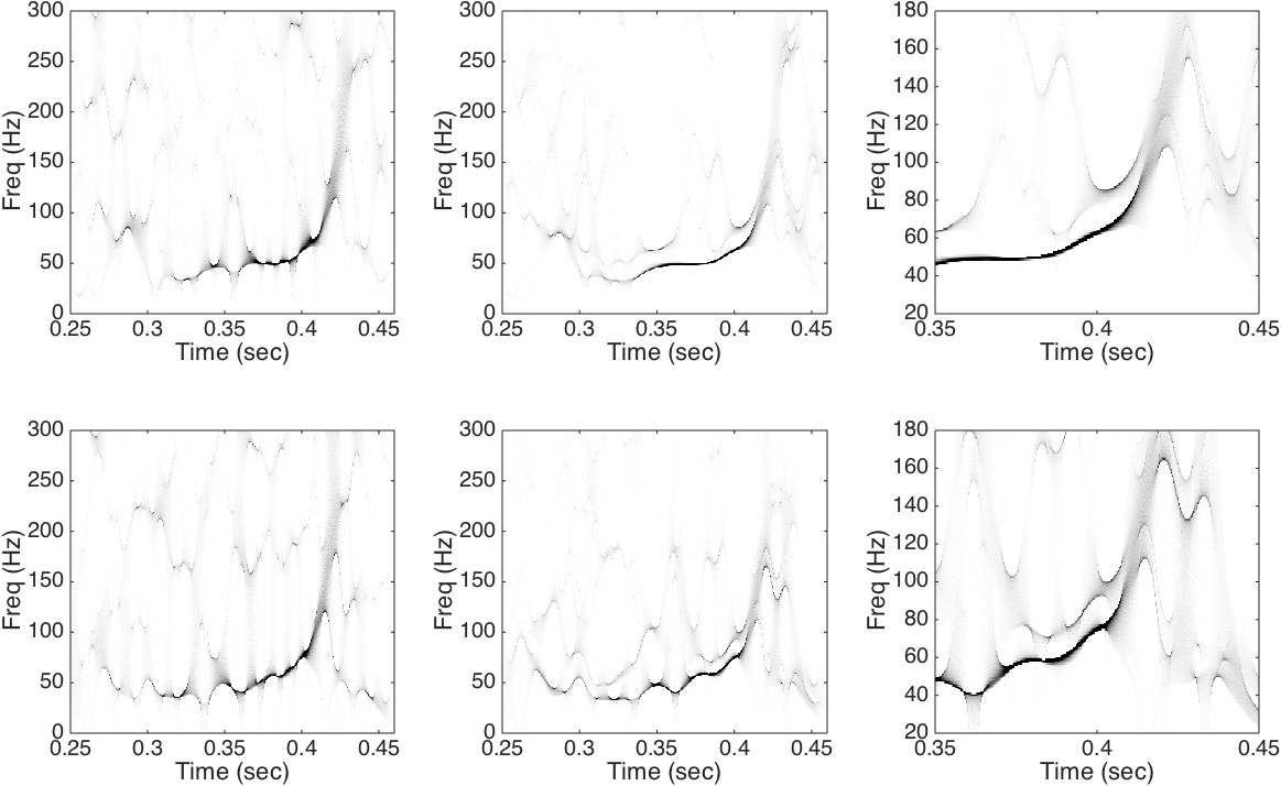
We now apply the Blaschke decomposition to analyze H1 and L1 signals, and show the TF representation determined by SST and the Blaschke TF representation. Since the amplitude of the signal varies, we apply the Blaschke decomposition with . The decomposition results are shown in Figures 13. We could see the chirp behavior after 0.35 seconds in both signals. The decomposed signals seem to have several “phase jumps”, for example around 0.3 second of the first decomposed component of both H1 and L1. These phase jumps could be explained by the inevitable noise in the recorded signal. The SST TF representations and the Blaschke TF representations of of H1 and L1 are shown in 14. For both H1 and L1, compared with the TF representation determined by SST, we could see that the Blaschke TF representation is sharper with less “background speckles” in the TF representation. Note that while the findings match the reported TF representations determined by CWT in [1], to further explore the results shown here and the potential of the proposed method, we need extensive collaborations with field experts, and the results will be reported in the future work.
5.5. Detecting Roots
In this last subsection, we show how the Blaschke decomposition reveals the roots of a given analytic function , when combined with the Poisson convolution.
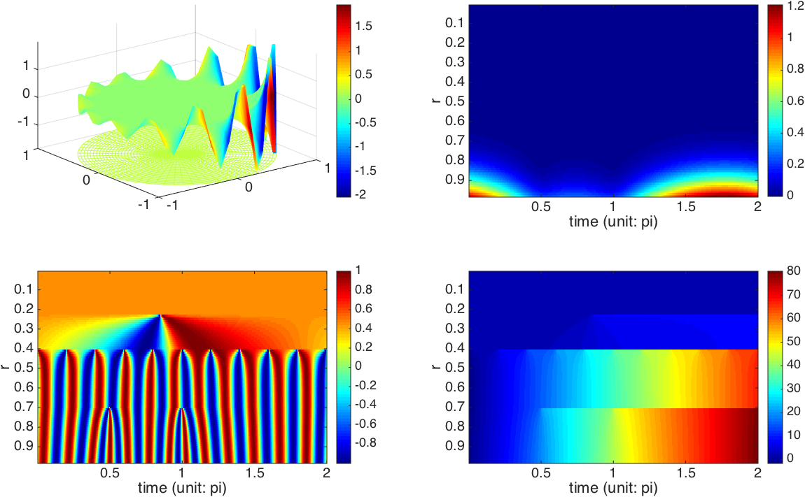
For , denote
where and the Blaschke decomposition of . Consider , where we have 10 roots on the circle of radius , 2 roots on the circle of radius and one root on the circle of radius . According to the discussion in Section 3.5, when we apply the Blaschke decomposition, we should see a “transition” from to , where , where and .
We sample points from uniformly on , and evaluate by the Poisson integral directly by evaluating the Rieman sum, where ranges from to with the uniform grid length . For each , we apply the Blaschke decomposition to evaluate . The results of the Poisson integral, the Blaschke decomposition are shown in Figure 15. Clearly, it is not easy to directly read the root location from . However, the root location information could be clearly seen from reading the “transition” in the phase of . Particularly, when the phase of increases up to , while the phase of increases only up to when and so on. The real part of , when indicates that oscillates with a fast-varying IF around time and , which reflects the roots at and . When , also oscillates with a non-constant IF, but the IF varies more slowly compared with the when . This observation reflects the fact that the non-constant IF is captured by the non-zero roots, and the farther the root is to , the faster the IF varies.
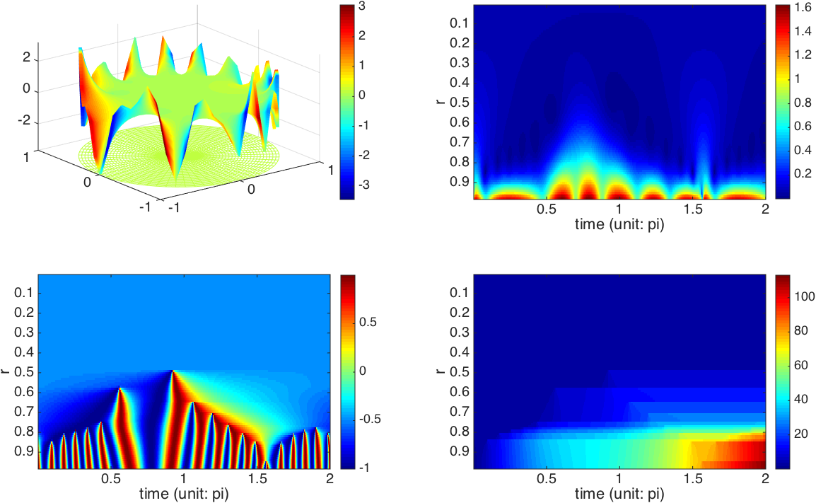
Next, we show the result for defined in (5). We sample at the sampling rate of 128Hz and ; that is, we sample points. The results of the Poisson integral, the Blaschke decomposition are shown in Figure 16. It is clear again that from reading the Poisson integral, little information about roots could be directly obtained. However, we could see several transitions across different in the phase plot of , which provides roots’ locations. While the exact relationship between roots and the analytic function satisfying the adaptive harmonic model is still open, this result shows the potential of applying the Blaschke decomposition to detect the roots of a given analytic function. For example, the nonlinear “strips” in the real of when changes might help quantify the relationship. The study of this relationship will be reported in the future work.
References
- [1] B. P. Abbott and et. al. Observation of gravitational waves from a binary black hole merger. Phys. Rev. Lett., 116:061102, Feb 2016.
- [2] F. Auger, E. Chassande-Mottin, and P. Flandrin. Making reassignment adjustable: The levenberg-marquardt approach. In Acoustics, Speech and Signal Processing (ICASSP), 2012 IEEE International Conference on, pages 3889–3892, March 2012.
- [3] F. Auger and P. Flandrin. Improving the readability of time-frequency and time-scale representations by the reassignment method. IEEE Trans. Signal Process., 43(5):1068 –1089, may 1995.
- [4] P. Balazs, M. Dörfler, F. Jaillet, N. Holighaus, and G. Velasco. Theory, implementation and applications of nonstationary Gabor frames. Journal of Computational and Applied Mathematics, 236(6):1481–1496, 2011.
- [5] Y.-C. Chen, M.-Y. Cheng, and H.-T. Wu. Nonparametric and adaptive modeling of dynamic seasonality and trend with heteroscedastic and dependent errors. J. Roy. Stat. Soc. B, 76:651–682, 2014.
- [6] C. K. Chui and H.N. Mhaskar. Signal decomposition and analysis via extraction of frequencies. Appl. Comput. Harmon. Anal., 40(1):97–136, 2016.
- [7] A. Cicone, J. Liu, and H. Zhou. Adaptive local iterative filtering for signal decomposition and instantaneous frequency analysis. Appl. Comput. Harmon. Anal., in press, 2016.
- [8] R. R. Coifman and S. Steinerberger. Nonlinear phase unwinding of functions. submitted, 2015.
- [9] I. Daubechies. Ten lectures on wavelets. SIAM, 1992.
- [10] I. Daubechies, J. Lu, and H.-T. Wu. Synchrosqueezed wavelet transforms: An empirical mode decomposition-like tool. Appl. Comput. Harmon. Anal., 30:243–261, 2011.
- [11] I. Daubechies and S. Maes. A nonlinear squeezing of the continuous wavelet transform based on auditory nerve models. Wavelets in Medicine and Biology, pages 527–546, 1996.
- [12] I. Daubechies, Y. Wang, and H.-T. Wu. ConceFT: Concentration of frequency and time via a multitapered synchrosqueezing transform. Philosophical Transactions of the Royal Society of London A: Mathematical, Physical and Engineering Sciences, 374(2065), 2016.
- [13] K. Dragomiretskiy and D. Zosso. Variational Mode Decomposition. IEEE Trans. Signal Process., 62(2):531–544, 2014.
- [14] P. Flandrin. Time-frequency/time-scale analysis, volume 10 of Wavelet Analysis and its Applications. Academic Press Inc., San Diego, 1999.
- [15] P. Flandrin. Time-frequency filtering based on spectrogram zeros. IEEE Sig. Proc. Lett., 22:2137–2141, 2015.
- [16] D. Gabor. Theory of communication. part 1: The analysis of information. J. Inst. Elec. Engrs. Part III, 93:429–441, May 1946.
- [17] G. Galiano and J. Velasco. On a non-local spectrogram for denoising one-dimensional signals. Applied Mathematics and Computation, 244:1–13, 2014.
- [18] J. Garnett. Bounded analytic functions. Pure and Applied Mathematics, 96. Academic Press, Inc., New York-London, 1981.
- [19] J. Gilles. Empirical Wavelet Transform. IEEE Trans. Signal Process., 61(16):3999–4010, 2013.
- [20] D. Healy. Phase analysis. talk given at the university of maryland. personal communication.
- [21] D. Healy. Presentation: Multi-resolution phase, modulation, doppler ultrasound velocimetry, and other trendy stuff. personal communication.
- [22] N. E. Huang, Z. Shen, S. R. Long, M.C. Wu, H.H. Shih, Q. Zheng, N.-C. Yen, C. C. Tung, and H. H. Liu. The empirical mode decomposition and the Hilbert spectrum for nonlinear and non-stationary time series analysis. Proc. R. Soc. Lond. A, 454(1971):903–995, 1998.
- [23] K. Kodera, R. Gendrin, and C. Villedary. Analysis of time-varying signals with small bt values. IEEE Trans. Acoust., Speech, Signal Processing, 26(1):64 – 76, feb 1978.
- [24] C.-Y. Lin, L. Su, and H.-T. Wu. Wave-shape function analysis – when cepstrum meets time-frequency analysis. submitted, 2016.
- [25] L. Lin, Y. Wang, and H. Zhou. Iterative filtering as an alternative for empirical mode decomposition. Adv. Adapt. Data Anal., 1(4):543–560, 2009.
- [26] S. Mallat. Group invariant scattering. Pure and Applied Mathematics, 10(65):1331–1398, 2012.
- [27] S. Mann and S. Haykin. The chirplet transform: physical considerations. Signal Process. IEEE Trans., 43(11):2745–2761, 1995.
- [28] M. Nahon. Phase Evaluation and Segmentation. PhD thesis, Yale University, New Haven, 2000.
- [29] N. Pustelnik, P. Borgnat, and P. Flandrin. Empirical mode decomposition revisited by multicomponent non-smooth convex optimization. Signal Processing, 102(0):313 – 331, 2014.
- [30] T. Qian. Intrinsic mono-component decomposition of functions: An advance of fourier theory. Mathematical Methods in the Applied Sciences, 33(7):880–891, 2010.
- [31] B. Ricaud, G. Stempfel, and B. Torrésani. An optimally concentrated Gabor transform for localized time-frequency components. Adv Comput Math, 40:683–702, 2014.
- [32] N. Saito and J. R. Letelier. Presentation: Amplitude and phase factorization of signals via blaschke product and its applications. JSIAM, 2009.
- [33] R.G. Stockwell, L. Mansinha, and R.P. Lowe. Localization of the complex spectrum: the S transform. Signal Process. IEEE Trans., 44(4):998–1001, 1996.
- [34] P. Tavallali, T. Hou, and Z. Shi. Extraction of intrawave signals using the sparse time-frequency representation method. Multiscale Modeling & Simulation, 12(4):1458–1493, 2014.
- [35] B. van der Pol. The fundamental principles of frequency modulation. Electrical Engineers - Part III: Radio and Communication Engineering, Journal of the Institution of, 93(23):153–158, May 1946.
- [36] G. Weiss and M. Weiss. A derivation of the main results of the theory of hp-spaces. Rev. Un. Mat. Argentina, 20:63–71, 1962.
- [37] H.-T. Wu, S.-S. Hseu, M.-Y. Bien, Y. R. Kou, and I. Daubechies. Evaluating physiological dynamics via synchrosqueezing: Prediction of ventilator weaning. IEEE Trans. Biomed. Eng., 61:736–744, 2013.
- [38] H.-T. Wu, R. Talmon, and Y.-L. Lo. Assess sleep stage by modern signal processing techniques. IEEE Transactions on Biomedical Engineering, 62:1159–1168, 2015.
- [39] Z. Wu and N. E. Huang. Ensemble empirical mode decomposition: a noise-assisted data analysis method. Adv. Adapt. Data Anal., 1:1 – 41, 2009.
- [40] S. Xi, H. Cao, X. Chen, X. Zhang, and X. Jin. A frequency-shift synchrosqueezing method for instantaneous speed estimation of rotating machinery. ASME. J. Manuf. Sci. Eng., 137(3):031012–031012–11, 2015.