Factorising the 3D Topologically Twisted Index
Abstract
We explore the path integration – upon the contour of hermitian (non-auxliary) field configurations – of topologically twisted Chern-Simons-matter theory (TTCSM) on times a segment. In this way, we obtain the formula for the 3D topologically twisted index, first as a convolution of TTCSM on times halves of , second as TTCSM on times – with a puncture –, and third as TTCSM on . In contradistinction to the first two cases, in the third case, the vector multiplet auxiliary field is constrained to be anti-hermitian.
1 Introduction
Recently, it has been pointed out a relation between 3D topologically twisted (TT) index of (Benini and Zaffaroni, 2015) and the entropy of supersymmetric black holes (Benini et al., 2015a; Hosseini and Zaffaroni, 2016) via the gauge/gravity correspondence. This is an interesting observation, that could potentially show a way to new insights into the microscopic structure of black holes, via careful analysis of relevant supersymmetric localisation results (Chung and Yoshida, 2016; Nedelin et al., 2016) and through holographic principles (Strominger and Vafa, 1996; Sen, 2008).
The 3D TT index of (Benini and Zaffaroni, 2015)11 1 Strictly speaking is a semi topological A-twist on (Witten, 1991). We will see what this means in a while. is a summation over magnetic fluxes –and integration over the Coulomb branch–
| (1.1) |
where , is the partition function of the Chern-Simons- SYM- matter theory (with semi-topological A twisting (Witten, 1991) over ), about a supersymmetric saddle point that includes, among non trivial values for other fields in the vector multiplet, the following background gauge potential
| (1.2) |
with being a generator having weight vectors in the co-root lattice of the corresponding gauge group . The contour of integration in (1.1) – denoted as JK – encloses the poles selected by a Jeffrey-Kirwan (JK) recipe (See (Jeffrey and Kirwan, 1993; Benini and Zaffaroni, 2015; Closset et al., 2015; Honda and Yoshida, 2015; Closset and Kim, 2016)).
Consistency with Aharony and Giveon-Kutasov dualities suggests the presence of the sum over 1 loop contributions about the fluxes . However, – at least to our knowledge – the origin of the latter sum, is not completely clear when integration over real path of fields is performed, by following the supersymmetric localisation method of (Pestun, 2012).
Let us explain the point made in the last sentence of the previous paragraph in more detail. Once we have defined a localising term for the vector multiplet sector, -( or -), we must specify reality conditions on the fields in the gauge multiplet: . The bosonic part of the aforementioned localising terms must be semi-positive definite and should vanish at specific set of classical configurations: the zero locus. The zero locus is the space of supersymmetric configurations that obey the specific set of reality conditions. The final result for the localised quantity is a sum over the zero locus. Potentials of the form (1.2) are not part of any zero locus – by themselves –, because they do not preserve any of the supercharges at disposal . In fact, the terms when evaluated at (1.2), are proportional to , independent on and consequently suppressed – with respect to the vacuum – when the naive "semiclassical" limit is taken 22 2 Configurations in the zero locus are the ones surviving the large limit. Notice that the gauge connections (1.2) can not depend on , due to the quantisation condition (GNO) for the fluxes . Hence the norm of the classical configuration (1.2), , is exponentially suppressed in any possible limit.. The issue then arises, as to how is it that is possible to get non trivial results from the backgrounds (1.2), in the "semiclassical" limit ?
Potentials (1.2) are supersymmetric when complemented with non trivial profiles of other fields in the vector multiplet. For instance, (1.2) preserve both and (Benini and Zaffaroni, 2015) when
| (1.3) |
Consequently, (1.2) + (1.3) is part of the zero locus of any combination with and arbitrary c-numbers. In (Benini and Zaffaroni, 2015) it was argued that the saddle points in question do contribute to the integration along the real path, even though they are not along the real line of integration, as in (1.3) is complex,. To show that they must contribute, the authors noticed the consequences of integration over the super manifold of zero modes . Specifically, they claimed that integration of along the line with (<0) was independent on . Given that the integrand is a function of then by defining the original "complex contour" gets shifted to the "real" one 33 3 Proper analysis (Benini and Zaffaroni, 2015; Benini et al., 2014; Benini et al., 2015b) reduces the integration over the supermultiplet of zero modes to the JK middle dimensional contour in the complex plane of bosonic expectation values ..
The supersymmetrisation of (1.2) by mean of (1.3) is not possible, should we had chosen to be hermitian. In the latter case there are two choices that supersymmetrise (1.2). Namely, there are two specific real but globally ill defined – they are non periodic – profiles for that do the work
| (1.4) |
Where stands for constant commuting generator and are arbitrary constants. For , the magnetic flux preserves and for , . Thence, naively speaking, one would say that (1.2)+(1.4) is part of the zero locus of the term with vector multiplet fields being real (hermitian). In summary, we have counted three possibilities, that putting aside global issues, could justify the sum over fluxes (1.1).
The reader could wonder whether there exists a constant value for to source the fluxes (1.2). In the case of 3D non TT index, like for instance the superconformal index, there is a constant profile for sourcing the fluxes (1.2) (Imamura and Yokoyama, 2011; Borokhov, 2004; Cremonesi, 2015) (See equation (21) of (Imamura and Yokoyama, 2011)). This potential contribution to the BPS conditions comes from terms in the superalgebra. However, these terms are proportional to and hence are not present in the case of the type semi-topological twisting. In conclusion, the only possible supersymmetriser for the the fluxes (1.2) in the topologically twisted analysis and without considering a complexification of , is something like (1.4).
Notice that (1.4) has explicit dependence on the time coordinate and is non periodic under . One way to solve this problem is to exclude a point out of the . In the latter case, the fluxes will be present and one could ask whether the TT index formula of (Benini and Zaffaroni, 2015) is recovered or not in this case. That will be one of the scopes of this work.
We will also explore whether the aforementioned formula for the TT index can be obtained out of dividing the into two open patches and . As naive intuition suggests, the result for the index will come after "glueing together", in the sense of (Pasquetti, 2012; Beem et al., 2014), the theories on and . We will start by attacking the problem in this way, because then is easier to take the limit on one of the blocks to recover the procedure mentioned in the previous paragraph. For that, necessarily, we will need to compute the partition function of 3D TTCSM on times an open segment .
Before entering in the bulk of the paper, let us explain in more detail one of the technical motivations that drove us to understand these issues. As the supercharges and are nilpotent (the and are our version of the supercharges and defined in equations (2.6) and (2.7) of (Benini and Zaffaroni, 2015)), the localising term used in (Benini and Zaffaroni, 2015), which in our conventions is
| (1.5) | |||||
| (1.6) |
with
| (1.7) |
is not only but -exact.
In virtue of (1.6), the localising action (1.5) is also -exact up to a total derivative. In fact one could have guessed this fact, from the known property – acting on gauge invariant objects –. Strictly speaking, the latter definition of is not ( resp. ) supersymmetric. In fact, from the nilpotency of and the RHS of (1.5) (resp. (1.6)) it follows that is (resp. ) supersymmetric only up to a total derivative.
The flux (1.2) when sourced by a complex value of , (1.2) + (1.3), belongs to the zero locus of (Benini and Zaffaroni, 2015). However, notice that the localising action (1.5) is not positive definite when is assumed to be complex. Nevertheless, this is not a problem to perform localisation. One of our conclusions, is that one can always define a exact term whose bosonic part is semi-positive definite under the reality conditions that define a given BPS configuration. In fact, we checked that (1.2) + (1.3) is not an exception to that rule.
The localisation term (1.5) is both, -exact (precisely) and -exact (up to total derivatives). Thenceforth, is also possible to use the two possible supporting real values of (1.2)+
(1.4) in such a way the magnetic fluxes become -BPS. There seems plausible to expect that with this real BPS configurations, there is not need to relax the reality condition for the auxiliary field in order to recover the sum over fluxes. What we are set to explore with our approach, is whether the final result for the path integral along the real contour will be the same or not obtained in (Benini and Zaffaroni, 2015) – they integrate over a complex contour–. In the least of the ambitions, our scope is to understand what are the assumptions or considerations that allow to recover their result.
Let us argue our point from a different perspective. From the reality condition for the bosonic fields in the gauge multiplet, it follows, that the bosonic part of
| (1.8) |
is positive definite. How could be possible that field configurations with finite energy density belong to the zero locus of the RHS of (1.5)? 44 4 In (Benini and Zaffaroni, 2015) (See also (Closset and Kim, 2016)) the authors define a ”semiclassical limit” in which the one loop determinant contribution cancels out the classical suppression. In the presence of the supermultiplet of zero modes . I would like to thank Francesco Benini for drawing my attention to this point. In this way, they provide an argument in favour of the presence of the sum over fluxes even when the usual localisation arguments seems to say the contrary when integrating over real fields (Honda and Yoshida, 2015). In this work an alternative way to explain the presence of the aforementioned fluxes – following the lines of the usual localisation program – was pursued.
From the point of view of the real saddle points (1.2)+(1.4) the answer to this question comes from the integration of the total derivative term , which is non trivial in this case. Evaluated on a magnetic flux and the corresponding scalar configuration that is needed to preserve either or , the integration of will provide a non trivial contribution that cancels the suppression contribution coming from (1.8). This contribution comes from the term .
This paper is organised as follows. In subsection 2.1 we recast the -superalgebra in terms of a redefined gauge potential, denoted as . This step, together with a proper selection of exact localising term, is essential to deal with the explicit time dependence of the zero locus profile for . It will also allow to absorb some of the effects of such a dependence with the help of gauge degeneracy. However, we stress that can not be absorbed completely Stuckelberg. What we meant to transmit in the previous sentence, is that we can eliminate only the explicit dependence on out of the quadratic operators to compute determinants upon, by a convenient choice of gauge and localising term. In other words, we will fix the imaginary part of in a convenient way, that allows to eliminate the aforementioned -dependent terms in a specific exact localising term 55 5 Semi-positive definiteness of the bosonic part of the exact localising term will not be affected at all by this choice.. It must be noticed that quadratic terms of the form , which are proportional to the magnetic flux, remain inert under such a gauge choice freedom. Such terms will play the role of in (Benini and Zaffaroni, 2015).
A point could be made on whether to relax the reality condition for would mean to diverse or not from the "real" contour of integration. However, the definition of "real" contour comes after gauge fixing is imposed, namely, functional integration is performed over physical degrees of freedom. As the imaginary part of is going to be fixed to a value, there will not be physical fluctuations along it and hence functional integration is performed over hermitian degrees of freedom. But this subjective point aside, the important point in favour of the approach to be followed here, is that semi-positive definiteness of the bosonic part localising term is not sacrificed along the path of integration. Next, we go on to define our localising terms for vector and matter multiplets, as well as Chern-Simons terms. We obtain the -localisation locus for our reality conditions and repeat the same analysis from the supercharge perspective.
Thereafter, we move on to compute the 3D TT partition functions on . We will show, that glueing together the partition functions on and results in the TT Index formula of (Benini and Zaffaroni, 2015).
Our reality conditions for the temporal component of imply that the moduli (the eigenvalues of its expectation value in the direction of a Cartan generator ) must be integrated along the real line; it also implies the annihilation of the VEV of which as will be shown, is the imaginary part of . The selection of the segment of integration for is not fixed a priori. Keeping this issue in mind, we move forward and using the periodicity properties of we define as the segment of integration. In fact the poles in due to the presence of a single pair of chiral-antichiral multiplets, appear with periodicity in the variable . Thence it is plausible to restrict integration to a single cell, as done in (Gadde et al., 2015) (in their case , only poles in the fundamental domain of the corresponding elliptic function are selected). In this way we take into consideration residues coming from a single pole in representation of a matter multiplet and not the full tale of images. This is, the remaining images of the selected pole do not signal the presence of additional matter content. In Appendix B.5, we illustrate how the result coincides with the JK prescription given in (Benini and Zaffaroni, 2015). To see that, one can see how to map the integral over the segment to the integration over a contour closed over the upper half of the complex plane and it is thenceforth reduced to a computation of residues. From this perspective it is clear to see the origin of the so called "boundary contribution" (Benini and Zaffaroni, 2015). We focus on the rank one case.
For completeness, we analyse the index of a massive deformation of with chiral-antichiral multiplets in the fundamental and such other pairs in the anti-fundamental. Even though we will only flavour a , the result of the integration is not vanishing in this case 66 6 The technical reason behind this suspicion is that the Vandermonde determinant would vanish evaluated at a point in the moduli space , should any pair of components and coincide with . . The summation over will spread the poles at of the fundamental matter multiplets in over the circumference of unit radius in such a way a non trivial result is obtained for the topologically twisted index which in our toy example goes like for large .77 7 The segment of integration crosses the poles in this case. Thenceforth, we define the integration as its principal value (PV).
2 The supercharges and
In this section we reconstruct the supercharges and in our conventions, with special emphasis in total derivatives. Because the zero locus background we are about to work with, does not preserve time homogeneity, it will be useful to redefine the gauge potential in a specific way, such that the trouble caused by time dependence of the aforementioned background gets absorbed by gauge degeneracy and a particular selection of exact localising terms. We call those terms "unorthodox". They have a positive definite bosonic action along the path of integration of interest. The exact terms proved to be a more convenient choice than the orthodox ones. In sake of completeness, we compare these "unorthodox" localising terms of vector and matter multiplet with the orthodox ones. All along this section we perform consistency checks that show that the redefinition mentioned above works perfectly. We define also "unorthodox" Chern-Simons terms as well as usual Chern-Simons terms. Finally we write down the that relates -results to -results and .
The first two subsections are intended to a reader interested in technical insights. If the interest is to get the general idea of our analysis, then we recommend to jump to Subsection 2.3 where the summary and scope of the analysis presented in the first two sections is given.
2.1 The supercharge in :
In this subsection we rewrite the -supersymmetry algebra in terms of a redefined gauge section that we denote as . Secondly, we define the corresponding -exact localisation actions for the vector and matter sectors, as well as Chern-Simons term to be used in . Complementarily, in appendix A we show that the bosonic and fermionic parts of the localising actions, with the original form of the algebra (2.9)-(2.1) 88 8 Before recasting it in terms of the redefined potential . , coincide with the corresponding ones in (Benini and Zaffaroni, 2015).
Let us start by a complexified gauge multiplet endowed with the following supersymmetry algebra
| (2.9) |
To us, the symbol will be exclusive to the operation of complex conjugation. What in (Benini and Zaffaroni, 2015) has been called we will call , namely
| (2.10) |
To us, is not an independent field but the complex conjugated of . The covariant derivative is absolute, namely it includes the gauge connection, the Symmetry background gauge connection, the spin connection, flavour background connection (See (A)). The killing spinor is commuting and hence is anti-commuting. More details on our conventions are given in Appendix A.
For convenience, let us show a property of the supersymmetry algebra (2.9) that will result useful later on when dealing with the zero locus that includes the background (1.4). Notice that (2.9) can be rewritten as
| (2.11) |
where is the fully covariant derivative but with a redefined gauge potential constructed out of and . The redefined potential coincides with except for the temporal component
| (2.12) |
is the field strength of .
The explicit form of the killing spinor (A.290), is cardinal in achieving the form (2.11). This is because in order to rearrange the spinor structure and being able to absorb the and derivative terms into the field strength term of the gaugino variation in (2.9) one must use that
| (2.13) |
together with the relations
| (2.14) |
In this paper the numerical indices will refer to flat space indices, so the reader should not confuse quantities such as with , the latter being obtained from the former by mean of the driebeins.
As for the complexified vector multiplet, we are going to be interested in the following reality conditions
| (2.15) |
Notice that the reality condition is imposed upon not upon . In terms of the condition is . However, as will become clear when computing one-loop determinants we are going to gauge fix and thence the imaginary part of will be non physical. The stand for a constant and hermitian generator, namely a real zero mode that we will call .
As for the matter multiplets and , the nilpotent algebra associated to reads
As already said for the gaugini,
| (2.16) |
where refers to (Benini and Zaffaroni, 2015).
For computational convenience we will rewrite (2.1) as
| (2.17) |
were is the fully covariant derivative but with the effective gauge potential defined in (2.12).
We are going to integrate the matter multiplets along the path
| (2.18) |
which guaranties positive semi-definiteness of our . As shall be argued upon in sections to come, we are interested in matter contents that do not create gauge/parity anomaly. This condition imposes a constraint on the gauge representation carried by the matter content (Redlich, 1984a; Redlich, 1984b).
Let us start by writing the localising term for the gauge multiplet
| (2.19) | |||||
| (2.20) |
In a while we will comment about (2.19) and its relation with the term used in (Benini and Zaffaroni, 2015), that we have written in the LHS of (1.5).
In subsections to come the non covariant form of the algebra (2.11) and the localising term (2.19) will be used to compute one loop determinants. This will prove to be useful at the technical level. Mainly because with the aforementioned form of the algebra and localising term, the explicit time dependence of the zero locus background mentioned in the introduction, (1.4), will be implicit.
From the term in the expansion of (2.19), and with the help of (2.11) is straightforward to get the bosonic part
| (2.21) |
It should be stressed that all equalities in this subsection do take into consideration total derivatives. Notice that with the reality conditions (2.15) this bosonic term is positive definite.
As for the fermionic part, one gets
| (2.22) |
with
| (2.23) |
From (2.22) we obtain the fermionic part of (2.19)
Notice that this expression is non covariant. The use of this non covariant form results convenient when computing 1-loop determinants. We stress that should be understood as covariant derivative that includes the magnetic flux potential felt by the effective charge of the corresponding gaugino component. Specifically, the spin connection part of the covariant derivative is included in the latter mentioned magnetic flux contribution. See appendix B.3 for further details in this issue.
In Appendix A.1 we show how to derive the localising action coming from (2.19) but by using the covariant form of the algebra (2.9). Is straightforward to check that the result for the action in the latter case is the same (2.21)+(2.1) but after substitution of (2.12). This coincidence, checks the consistency of using the algebra in terms of the redefined potential (2.11) instead of the usual one in terms of (2.9).
It is also possible to use the orthodox localising term, the one used in (Benini and Zaffaroni, 2015) for instance, which in the conventions used in this paper is given by
| (2.29) |
| (2.30) | |||||
| (2.31) |
with and . Trace over the gauge indices is assumed in (2.30) and (2.31). It is straightforward to show that after replacing the expression for the redefined gauge potential in terms of , (2.12), in (2.31), one obtains the covariant form of the localising action. Namely, the localising term (2.29) worked out with the covariant form of the algebra (2.9)
| (2.32) |
Again, this coincidence checks the consistency of using the algebra in terms of the redefined potential (2.11) instead of the covariant one (2.9).
As one could expect a priori, the difference between the localising term (2.19) and (2.29) is the - exact term
| (2.33) |
which, naively, in virtue of the localisation argument, means both localising terms are set to compute the same observables. However one must not forget that the for the reality conditions (2.15), the bosonic part of the localising term to be used here, (2.19), is positive definite, meanwhile the bosonic part of (2.29) is not.
Next, the same analysis will be performed for the matter sector of the theory. Let us define the following localising term
| (2.34) |
In appendix A.2, it will be seen how this localising term differs from the one used in (Benini and Zaffaroni, 2015), by using the covariant form of the algebra (2.9) and (2.1). The difference being a exact term, as shall be seen below and thenceforth both localising terms are set to compute the same observables.
The expansion of (2.34) under the redefined form of the algebra, (2.11) and (2.17), is given by the sum of the following bosonic and fermionic terms
| (2.35) | |||||
| (2.36) |
The saddle point expansion of these Lagrangians about the localising locus will coincide with the one of (Benini and Zaffaroni, 2015). Notice the presence of the term . This term provides the flux dependence that in (Benini and Zaffaroni, 2015) comes from the complex value of . Specifically the zero locus condition will fix to the density .
To show the difference of the localising term (2.34) with the orthodox one, the one used in (Benini and Zaffaroni, 2015), let us write down the latter one in our conventions. The orthodox localising term for matter in the conventions of this paper is given by the super derivative
| (2.37) |
where the algebra has not been defined yet. We postpone the writing of until next subsection, equation (2.66), in order not to make too clumsy the presentation in this subsection.
| (2.38) | |||||
| (2.39) |
With the use of the redefinition of in terms of (2.12), this expansion presented before coincides with the expansion in terms of the original form of the algebra (2.9) and (2.1) which is given by
| (2.40) | |||||
| (2.41) |
Again, this coincidence checks the consistency of using the redefined form of the algebra (2.17). Let us take a moment aside to comment about the importance of total derivatives when dealing with BPS configurations of the kind (1.4). Notice that should one discard the total derivative term in (2.40) the quadratic expansion about the zero loci of the form (1.2)+(1.4) would not depend on the fluxes . Indeed, discarding such a term would be a mistake, because its integration over is non trivial. This is the reason why using the form (2.38) instead of (2.40) is advisable. However notice that (2.40) has an explicit dependence on that will give rise to an explicit dependence on in the quadratic expansion. Such a dependence can be absorbed by adding up a exact term. The final and homogeneous in time quadratic operator expansion would be coming from the new - exact localising term (2.34) whose bosonic part has been written in (2.35).
The difference between the super-derivative localising term (2.37) and the one to be used to compute one loop determinants (2.34), is the exact term
| (2.42) |
so in virtue of the localisation argument both localising terms are set to compute the same observables. However, as already argued (2.34) is the most convenient choice for our purposes. The exact difference (2.42) follows directly from equation (A.315).
We can also define the "unorthodox" supersymmetric Chern-Simons term
| (2.43) |
is supersymmetric under (2.11). The variation of the bosonic CS part is a multiplication of by a linear combination of and . The variation of the fermionic term, specially because it involves only the product 1010 10 From the algebra (2.11) is easy to see that the variation of involves only a linear combination of and ., is again multiplied by the precise linear combination of and that cancels the variation of the bosonic term. As a classical contribution, the Chern-Simons term will not affect the 1-loop determinants, it will only provide an extra on shell value. This unorthodox CS term proved to be more natural to our analysis than the orthodox one. Its variation gives the total derivative
| (2.44) |
For completeness, we write down the orthodox Chern-Simons term which is symmetric under the covariant form of both algebras and . In our conventions it is given by
| (2.45) |
Its total derivative variation is
| (2.46) |
We will also use the mixed CS term
| (2.47) |
with being the component along of a gauge background connection associated to a topological symmetry (See subsection 2.1.3 of (Benini and Zaffaroni, 2015) for more details). In (Benini and Zaffaroni, 2015) other modified Chern-Simons terms are written. However (2.47) is supersymmetric by itself and it is enough to our purposes. For completeness we write down its total derivative variation
| (2.48) |
The Localisation locus
In this subsection the locus consistent with the reality conditions (2.15) and (2.18) is defined. This information plus gauge fixing conditions, specify the path of functional integration. At last, it is evaluated the localising term for vector and matter sectors around the aforementioned locus.
We start from the -BPS conditions
| (2.49) | |||||
| (2.50) | |||||
| (2.51) | |||||
| (2.52) |
which reduce to
| (2.53) | |||
| (2.54) |
Before imposing reality conditions on the fields, this is the most general zero locus condition. From reality conditions and (2.83)
| (2.55) |
From (2.83), and again the reality conditions (2.15), it follows the set of equations
| (2.56) |
This is the same form of the Bogomolnyi equations reported in equation (9.7) of (Kapustin and Witten, 2007). In the first equation we can substitute by because .
In Appendix (B.1) we elaborate on how one arrives to the non vanishing part zero locus solution on the segment
| (2.57) |
We will use the following gauge potential parameterisation all along this paper
| (2.58) |
At this point we can evaluate the classical Lagrangian densities on the zero locus. From equations (2.21) and (2.43)
| (2.59) | |||||
| (2.60) |
where . In our conventions if and are Cartan generators then . Finally we are ready to write down the classical contributions
| (2.61) |
We will also use the contribution of the topological factor (2.47)
| (2.62) |
to absorb inconvenient phase factors of the same form, like for instance .
2.2 The supercharge in :
In this subsection we first reconstruct the supercharge that anti-commutes equivariantly with the chiral one . Namely
| (2.63) |
where the gauge covariant Lie derivative in the RHS is defined as
| (2.64) |
for every field except for the redefined gauge potential , for which the action is the following one
| (2.65) |
Notice that in the RHS of (2.63) there is not gauge transformation with as parameter. This is because such a gauge transformation is implicit in the hatted potential action upon the corresponding fields. It is straightforward to find, that the super-transformations for the gauge multiplet are given by
| (2.66) |
In this subsection, we will only present the analysis in terms of the redefined potential . The covariant form of the supercharge can be obtained by using the definition (2.12) and the identity (2.14). In Appendix A.3 we compute the orthodox localising term in terms of the covariant form of .
The unorthodox localising term that will be used to compute one loop determinants for the vector multiplet is
| (2.67) | |||||
which after expanded gives the following bosonic and fermionic terms
| (2.68) | |||||
| (2.74) |
In Appendix A.3 we present the analog results that come after use of the orthodox localising term.
As for the matter multiplets the transformations are
| (2.75) |
The localising term to be used in the computation of one loop determinants for matter is
| (2.76) |
whose expansion gives the following bosonic and fermionic parts
| (2.77) | |||||
| (2.78) | |||||
One possible invariant Chern-Simons term to use is
| (2.79) |
whose variation gives the following total derivative
| (2.80) |
The total derivative variation of the covariant Chern-Simons term (2.45) is in this case
| (2.81) |
The total derivative variation of the modified Chern-Simons term (2.47)
| (2.82) |
Following the procedure already detailed in the previous subsection one finds the following zero locus conditions
| (2.83) | |||
| (2.84) |
For the matter multiplet one arrives to based on arguments used in the case of in Appendix B.1. For the vector multiplet and for the reality conditions used in this work, the conditions for the bosons become together with the Bogomolnyi equations
| (2.85) |
The red colour plus sign is written to highlight the difference with the locus conditions (2.56). Repeating the analysis of the previous subsection one obtains to the following form of the locus
| (2.86) |
where again the weights of the generator are GNO quantised and in the Cartan of .
Next we are in conditions to write down the classical Lagrangian densities evaluated on the zero locus. From equations (2.68) and (2.79) we get
| (2.87) | |||||
| (2.88) |
The classical on shell action values are
| (2.89) |
2.2.1 The transformation :
For the reality conditions (2.15) the following transformation maps to and , in the following way
| (2.90) | |||
| (2.91) | |||
| (2.92) | |||
| (2.93) |
and
| (2.94) | |||
| (2.95) |
The complex conjugation plays a role even when supposing the reality conditions (2.15). This is because the supertransformations of real fields will be complex, as one can easily notice by observing carefully the RHS, for instance of (2.11). This transformation can be used as a tool to check the matching of and supersymmetric of exact objects, like for instance the localising actions and their variations. Notice that resembles a transformation, but it is not because and , for instance, are a priori independent degrees of freedom, not complex conjugated to each other.
2.3 What is localisation computing?
This subsection is a summary of results presented in the previous ones. In particular we will stress what are the actions that and localisation integrate out. Both of these localising actions are equivalent up to total derivatives 1111 11 The orthodox ones. The unorthodox ones are not related by a total derivative as we have already seen. The difference between the orthodox and unorthodox terms are and in both ”chiral” and ”antichiral” sectors, respectively. The addition of these exact terms spoils the total derivative relation between ”chiral” and ”antichiral” localising terms. as we have already seen. What we will further remark, is that when placed on a manifold with boundaries, topologically twisted Chern-Simons-matther theory (TTCSM) has two possible versions to be used. We will call these versions as and - TTCSM respectively.
In the end of this subsection we explore how to supersymmetrise the modified Chern-Simons terms on segments, in a gauge covariant way. For that, an additional set of boundary conditions will need to be imposed upon the vector multiplet. As will be discussed in a while, this set of boundary conditions guaranties well definiteness of the variational problem on times a segment in the vector multiplet sector. We will also identify and discuss about a set of boundary conditions for the matter sector that will guaranty both supersymmetry and well definiteness of the variational problem on times a segment.
We can define a exact term that differs from the Lagrangian of SYM Lagrangian on times a segment by a total derivative. Let us explain this last point in more detail. For us, SYM Lagrangian density is defined as
| (2.96) | |||||
| (2.97) | |||||
where trace over the gauge indices in the first line, is implicit. To study the variations of one can use the following identities
| (2.98) |
where and are the orthodox localising terms, which for the vector multiplet are (2.29) and (A.327) respectively, and for the matter multiplet are (2.37) and (A.333) respectively. The currents can be divided into vector and matter part
| (2.99) |
As for the vector currents, one gets
| (2.100) | |||||
| (2.101) |
As for the matter currents one gets
| (2.102) | |||||
| (2.103) |
Relations (2.98) are of special interest, because the (resp. ) ( resp. )-exact term is nilpotent with respect to (resp. ). Consequently, total derivatives do not come out in their SUSY variations. Thence from these equations one immediately reads out the and variations of the Lagrangian .
Thence the and variations of the and actions are
| (2.104) |
The and localisation are set to compute not the partition function of , but instead the path integral of the actions
| (2.105) | |||||
The actions are precisely the orthodox localising terms. The consequence, at the technical level, of the total derivatives that define in terms of is to cancel the classical on shell value of evaluated on BPS configurations with finite flux and henceforth, the latter are not suppressed in the large limit (This cancellation follows through in the same way already explained in the introduction).
We can write down the localising Lagrangian densities associated to (2.105) without explicitly writing the total derivative terms: they are simply the orthodox localising terms.
Summarising, we write down the two different choices of localising terms – from the results in the previous subsections–
The the supersymmetry variations of are zero follows from the nilpotency property . The option to the left (resp. right) in each parenthesis refers to the vector ( resp. matter) multiplet. We must stress that the first and second big parenthesis in each of the lines in (2.3), are not the same. The difference being a (first line) and (second line) exact terms as already shown in previous sections. In the first line for instance such a exact difference is given by
| (2.109) |
As we have already stressed several times in previous subsections, the first option that we have called before "unorthodox" terms, is the convenient one for our purposes and due to technical issues. The currents that define the difference between the Q-exact term and the SYM action that we wrote above, are coming from the "orthodox" terms, but the analog ones coming from the "unorthodox" terms can be easily deduced from the results presented in previous subsections.
To stress differences, we will discern between the 3D TT exact action coming from and by using the following terminology
- •
The theory we will call 3D -TT theory.
- •
The theory we will call 3D -TT theory.
For completeness let us collect here the Chern-Simons terms that define two possible , that were defined in the previous section as
and move on to analyse their variations. Is easy to see that the component coming from the variation of the matter-Chern-Simons term (2.47) is zero (the super variation of these terms is again of the form ) and thence this term does not suffer from supercharge leaking through the extrema of the corresponding patch or .
As for the "unorthodox" Chern-Simons term variations (2.43) and (2.79) there is a non trivial component, that can be easily inferred out of the variations (2.44) and (2.80) to be
| (2.113) |
These contributions can be cancelled with the addition of the following boundary action to the modified CS terms
| (2.114) |
However this term breaks gauge invariance. In (Yoshida and Sugiyama, 2014) the reader can find two procedures to tackle this issue. However, we will solve this problem in a different way.
First we remind that in taking the large limit in localisation we must redefine every field in the theory in the following way
| (2.115) |
where denotes the profile of the field in the BPS state of consideration. Before continuing we stress that apart from the presence of boundary contributions coming from the variations (2.113), no constraint is needed over (2.115) in order to preserve supersymmetry, because we have defined density Lagrangians whose supersymmetric variations vanish trivially.
However, as we want the Chern-Simons term to be supersymmetric, we will impose (2.113) to vanish at and and in consequence we are forced to analyse the consistency of such constraint with the supersymmetry algebra of interest or . Specifically, when is either ( or ) we will always consider
| (2.116) |
Thenceforth, should we impose at the boundaries of the following Dirichlet (D) conditions upon the fluctuations
| (2.117) |
the variation of the Chern-Simons terms (2.113) vanish. After imposing (2.117) for and and given the fact that the are supersymmetric by definition, in order not to break the superalgebra transformations (2.11) and (2.66) at the boundaries and we must impose the - conditions for every other fluctuation in the vector multiplet. This guaranties that the full off shell fields preserve super-transformations at the boundaries and once (2.117) is imposed. For the matter multiplet this is not necessary. In a while, we will see what are the consequences of imposing the -conditions at the boundaries.
So far we have only commented on the conditions that are needed to guaranty supersymmetry on times an interval . Let us pause to comment on how the aforementioned conditions also ensure a well defined variational problem on . First, let us refer to the vector multiplet linear fluctuations that will be denoted as . The boundary term variations of the vector multiplet action (2.19) and Chern Simons (2.43) actions once the EOM’s are demanded, integrate to zero after imposing Dirichlet boundary conditions upon off shell fluctuations. Namely, should we demand the variational problem for the vector multiplet sector is well defined as it stands, because the boundary terms integrate to zero.
The variation of the matter multiplet action (2.34) is a total derivative once the EOM’s are imposed. This total derivative variation integrates to zero on , if we impose the following boundary condition
| (2.118) |
on fields in the matter multiplet and their variations . The choices + and - are independent and in the next section they will be called even and odd respectively. Clearly the + choice guaranties the boundary variations at both extrema to cancel each other, together with the -conditions for the vector multiplet. The choice - does the work too, because the boundary terms are quadratic in matter background - fluctuations as one can directly infer out of (2.35) and (2.36). The variational problem on times the segment of length is well defined with the aforementioned conditions. Clearly (2.118) is consistent with supersymmetry algebrae (2.17) and (2.75) and in consequence they preserve supersymmetry. We finish this section by noticing that the D-conditions
| (2.119) |
also guaranty the variational problem is well defined for matter. However, we will mainly use (2.118), unless we explicitly say we use (2.119).
Two variational problems on
VP-I) To have a well defined variational problem on , we take either the limit of the action coming from the Lagrangian density
| (2.120) |
or of that comes from
| (2.121) |
together with the D-conditions for the vector multiplet fluctuations and (2.118) at . The previous limit produces a well defined variational problem on . However, an important fact we can not overview is that, for instance with , has stationary points that break the periodicity of at , as for instance the BPS configuration (2.57). The fact such solutions break the topology of forces the exclusion of a point out of the in order to have them into consideration. In fact (2.57) is a solution of the EOM’s that come from the "unorthodox" localising term (2.19)(+(2.43)), specifically from (2.21)(+(2.43)) discarding back-reaction from the matter sector and gaugini which are zero in this background. It is easy to see that the linear differential of (2.21) vanishes identically upon evaluation on (2.57). The variation of the CS (2.43) and interaction terms between the vector and matter multiplets, under a variation of the bosonic vector multiplet fields , integrates to if
| (2.122) |
is imposed at the point of . For instance, the total derivative that results (together with an interaction term in the EOM’s times ) from the variation of the term proportional to in (2.38), integrates to if . In conclusion, (2.57) is a minimum of the "unorthodox" with , under variations that obey the Dirichlet condition at the point of . However (2.57) with is not periodic on and in conclusion is singular with . On the
- •
matter sector we can again impose Dirichlet boundary conditions (2.119)
- •
or the less restrictive condition (2.118).
Notice that the latter set of conditions allows for discontinuity of the fields at .
The weak point of this approach is that in order to keep non trivial fluxes one must sacrifice continuity at the point where the D-condition is imposed for the off shell fluctuations . In other words, in this case we must consider with the point excluded.
VP-II) We can define a different variational problem on that allows for the presence of minima that are non trivial BPS configurations, with flux on and respect the periodicity of . First we define the Lagrangian density
where ( resp. ) is ( resp. ) supersymmetric up to a total derivative that integrates trivially with the forthcoming conditions. Second, we define matching (continuity) conditions from one side to the other of the junction points
| (2.126) |
The matching conditions (2.126) select the following BPS configurations
Additionally, we demand the off shell variations to vanish at the junction points and , namely
| (2.130) |
Out of the equations labeled in (2.3), it is straightforward to check that the D-conditions (2.130) guaranty that the total derivative part of the off shell variations of integrates to zero on . Of course (2.115) needs to be satisfied too and in the case of the matter multiplet we impose on top of that
| (2.131) |
When condition (2.131) is imposed on top of (2.115), it kills any possible non trivial BPS configuration coming from the matter sector. In subsection 3.1 we will show how (2.131) is consistent with the previously mentioned set of boundary conditions for the matter sector: (2.118). In fact the results in subsection 3.2, allow to quantise this last variational problem by demanding even (resp. odd) condition (2.118) on top of (2.131) when ( resp. ). In subsection 3.3 it will be shown that the quantisation of (2.3) mentioned in the previous sentence, results in the sum over fluxes that we have called 3D TT index on , after localising to the BPS configurations (2.3). In the very end, supersymmetric localisation reduces the problem to quantum mechanics on with Dirichlet conditions on antipodal points.
2.4 The "complex" path of integration: The proper localising term
In this subsection we write down the localising term for the vector multiplet that must be used when the path of integration is the one proposed in (Benini and Zaffaroni, 2015). As for the matter multiplet one can use any of the localising terms written down in previous sections. The reality conditions for the vector multiplet in this case are
| (2.132) |
The right localising term to use is
| (2.133) | |||||
We say is the right one, because it has positive definite bosonic part along (2.132). The difference between (2.133) and (2.19) is the following exact term
| (2.134) |
The expansion of (2.133) with the form of the algebra (2.11) gives the following bosonic
| (2.135) |
and fermionic parts
| (2.136) |
Notice that only a pair of fermionic DOF’s remains dynamical in this localising action. This is reflection of the cohomological cancellations, in fact these are the DOF’s orthogonal to . When computing the one loop determinants, we will see how this fact is cardinal to obtain the correct result given in (Benini and Zaffaroni, 2015). The and are fermionic zero modes of (2.136). In order no to get a non vanishing result we must not integrate over and .
We can also use the localising term analog to the one used in Appendix A.1 (A.306), which as explained there, must not be confused with (2.133), namely
| (2.137) | |||||
| (2.138) |
After expanding this term with the help of the covariant form of the algebra (2.9) we obtain similar bosonic and fermionic parts as in (2.135) and (2.136) respectively
| (2.139) |
The determinant of the Dirac matrix in (2.4) is formally zero, because the mode are zero modes of the corresponding localising operator. In order no to get a non vanishing result we will not integrate over and .
The bosonic term (2.139) is not positive definite under the conditions (2.132) but instead under
| (2.145) |
We prefer to use the path of integration (2.132), thenceforth (2.133) is the proper choice and from now on when we refer to the complex path of integration we intend the use of that localising term.
The zero locus configurations in the path (2.132) are given by the fluxes on
| (2.146) |
where
| (2.147) |
is the combination of a couple of GNO quantised elements, coming from the real configuration for (2.57) and coming from the complex configuration for
| (2.148) |
From now on we will focus on the real path of integration introduced in previous sections (2.15). However, the computations of one loop determinants for the matter sector are equivalent in both paths of integration (2.15) and (2.132). The subtle difference comes out in the computation of the vector multiplet one loop determinants. For completeness of analysis, in Appendix B.4 we compute the one loop determinants of the vector multiplet in the complex path (2.132), namely with the terms (2.135) and (2.136).
3 The 3D TT Index on : "real" vs "complex" path
In this section we write down the two path integral representations of the index that we promised. The first representation will be a "product" of two blocks. The two blocks being the partition functions of the TT theory on with being a semicircle 1414 14 The and TT theories localise to the same result when placed on times an open segment with the boundary conditions we are choosing.. There will be two possibilities of matching the fluxes from one side to the other. If the match from to is continuous, then we are quantising the variational problem VP-II. The latter, is a functional integration over the real path of fields of the theory (2.3) on . In this way we reproduce the result of (Benini and Zaffaroni, 2015) but integrating along a section of hermitian fields.
Thereafter, we write down a second representation: The path integral of, either or -TT theory on which is nothing but the quantisation of the variational problem VP-I on . In this way we conclude that in order to have coincidence between the integration along the "real" and "complex" paths of integration when we integrate the theory VP-I along the former path 1515 15 Along the complex path of integration in order to have fluxes, we just need to consider the regular BPS solutions (2.148) as done in (Benini and Zaffaroni, 2015)., we must consider contributions coming from real BPS configurations that do not belong to but to .
3.1 Functional space of integration: boundary state on
The main scope of this subsection is to define the functional space of integration we will use to compute the gaussian path integrals defining the one loop determinants needed in the "semiclassical" limit of localisation. On passing by, we highlight one of the positive outcomes of considering localising density lagrangians with vanishing supersymmetric variations (even taking into consideration total derivatives): The wave function of a boundary state.
Let us start by thinking about what we called the "3D TT theory"
| (3.149) |
defined on . The analysis for the TT theory is completely analog and hence can be reproduced following the same line of reasoning. In this subsection we consider the Chern Simons coupling to vanish, namely .
The action defined by the Lagrangian density above (excluding the Chern-Simons term whose variation will be discussed below), is invariant and the domain space is compact; consequently we are not forced to impose boundary conditions for the vector and matter multiplets. Namely supersymmetry and finiteness of the action are already guarantied. The integral over will be a functional of the set of boundary conditions we choose.
Let us denote the set of asymptotic behaviours we would like to impose about or by
| (3.150) |
with being the localisation "Planck scale" parameter and an index running over the set of saddles. Equation (3.150) can be interpreted as a branching of the boundary asymptotic behaviour at or in terms of the redefinition of fields used in order to take the semiclassical limit of localisation.
Let us denote by the path integral of and by the same functional integral, but after imposing the boundary conditions at for the integrated fields. When the localisation limit is performed upon , as summarised in this equation below
| (3.151) |
one remains with a functional of the -BPS charges and the boundary data . Notice that we refer to as an asymptotic behaviour. This is because the boundary data encoded in could be given by values of the fields but also by the values of - derivatives of the fields at and . The function is called the wave function of the boundary state: the state defined by the boundary conditions . In bra and kets terminology, is the saddle approximation to around -th BPS state with boundary data .
From now on, we will use the following terminology
- •
The bras of , := - wave functions of the boundary state .
- •
The kets of , := - wave functions of the boundary state .
Notice that we have omitted the suffices and in the bra and ket respectively. The bra and ket denote the partition function with domain and respectively; however, at some points we will use the suffices in order to avoid confusion.
The partition function on is recoverable out of the space of wave functions of boundary states. In fact, when we take the Chern Simons coupling to vanish (), the partition function on is
Wave function of boundary state
Let us illustrate with a rather simple example of the matter multiplet sector with r-charge and without flavour charges around a BPS solution (2.57) with flux
| (3.152) | |||||
| (3.153) | |||||
| (3.154) |
with
| (3.155) | |||||
with 1616 16 Note that our is the one used in (Benini and Zaffaroni, 2015). and
| (3.159) | |||||
| (3.160) |
Notice that in our convention, , whereas for the convention used in (Benini and Zaffaroni, 2015), 1717 17 The lowers the eigenvalues of the part of , namely the magnetic Laplacian on , from by , namely to . In contradistinction, it raises the magnetic level of the spin spherical harmonics by a unit, namely from to . The opposite statement can be said for . In summary, the action of the operators on magnetic spherical harmonics can be represented as with being the spin spherical harmonic in . . The boundary term in (3.154) has two components, the first one, comes from the partial integration that was performed in order to arrive to the more appealing form of the action (3.153) and the second comes from the specific term used to localise, which in this case was (2.35)+(2.36). Notice that the total derivative coming from the bosonic part of (2.35) integrates trivially on . Our boundary conditions guaranty the vanishing of the aforementioned boundary term.
We define the space of functional integration on to be
| (3.174) |
A very important point is that for the even and odd quantisations (3.174), and , the boundary term (3.154) vanishes identically.
We have omitted the direct sums that act upon each of the internal factors in the direct products inside the first parenthesis, in order not to make too clumsy the notation. The is defined as follows
The relative differences between the magnetic level of the spin spherical harmonics in (3.174) is determined from consistency with the supersymmetry transformations (2.17). For instance from the part of the algebra (2.17) and after the redefinition (2.115) one gets
From the third line we conclude that when the magnetic level associated to the fluctuation is assumed to be , the one associated to is and the one associated to is . Then by analysing the of algebra (2.75) and after the redefinition (2.115) one closes the cycle to magnetic levels written in (3.174) after supposing the level of to be .
The operators and have the following non vanishing expectation values on the relevant spin spherical harmonics in (3.174)
| (3.192) |
The basis vectors being normalised as follows
| (3.193) | |||||
| (3.194) |
Under these orthonormalisation conditions the sandwich of and between states with different labels , vanishes.
Let us explain the meaning of the ’s in () in the case . The meaning of the in the alternative case follows straightforwardly. For instance, when , there is not "chiral" mode but there is "antichiral" mode (Benini and Zaffaroni, 2015). In this case the ’s at the positions , and of the corresponding matrix in () denote the absence of these components due to the lack of "chiral"(resp. "antichiral") mode . Notice that the determinant of the fermionic Dirac matrix in the first line of (), coincides with the eigenvalue of the bosonic operator (3.192) . As is the bosonic operator (complex scalar) action (3.153) and the Dirac operator () is the fermionic counterpart in (3.153) one could naively conclude that bosonic and fermionic determinants of (3.153) should cancel each other out due to the fact mentioned in the previous sentence. However, as will be shown in a while, cancellation between bosonic/fermionic determinants does not follow, due to the lack of "chiral/antichiral ground state" at level . The dots in the second and third line of () represent the absence of such "chiral/antichiral" ground state at the respective spin level (Benini and Zaffaroni, 2015).
Let us continue with our example of boundary state. Should we select the following boundary conditions at both and
| (3.195) |
the functional space (3.174) collapses to that single state with the following semiclassical distribution density
| (3.196) |
where by we mean the expectation values posted in (3.192). By and in (3.195), we mean the asymptotic behaviour of in a vicinity of and . Notice that the selection of the mode in (3.195), determines not only the value of but also their derivatives at and .
On the and KK mode space
The KK basis states in spaces (3.174) are not physical when one works with hermitian fluctuations (because they are complex). This is the case of the vector multiplet fluctuations. However these complex KK states can be used in any case, to compute the determinant of . It is convenient to work with these modes, because they are eigenstates and thence further diagonalisation procedures are not needed. The complex space spanned by these complex basis states is
| (3.197) |
In the case of hermitian fluctuations one needs to restrict to the subspace defined by
| (3.198) |
which is the real vector space
Notice that when (3.1) contracts to
| (3.202) |
In (3.1) and (3.202) one can further restrict to or or a combination of them by imposing Dirichlet or Neumann boundary conditions upon the fluctuations at and . Specifically
As already explained at the end of the previous section, we will use the first of these restrictions for the vector multiplet case, in order to annihilate the boundary variations of the modified Chern-Simons term in a gauge invariant way. We stress that, for the matter multiplet, the selection of or KK modes does not have to do with preservation of supersymmetry, even though both choices preserve supersymmetry. In previous sections we argued that the selection of one of the quantisations even/ odd has to do with the correct definition of variational problem. In this section the evident consequence of the choices even/ odd is the cancelation of the boundary term (3.154). Moreover, let us stress, that in order to have an orthonormal basis of KK modes on the interval we must choose either even or odd quantisation but we can’t have both at the time. In the latter line of thought, the choice of even or odd is a freedom we have, in order to define the functional space of integration .
3.2 3D TT index on times an interval
In this subsection we write down the relevant one loop determinants on and . The functional integration of (3.153) (together with integration over the boundary conditions ) over the functional space (3.174), is easy to perform with the use of (3.192). The final result for the one loop determinant around the BPS configuration is
| (3.210) | |||||
To arrive to this formula above one must write down the quotient between the fermionic
| (3.215) |
and bosonic determinant (inverse of the partition function of the complex scalar)
| (3.216) |
The determinants (3.215) and (3.216) are computed out of the relevant matrix elements, which are given in equations () and (3.192). In this case . Notice that we have dropped some minus signs. Those signs can be absorbed by the transformations which are involutions of the set of KK modes and weights we are going to multiply over. At this point, is straightforward to check that
| (3.217) |
To obtain (3.210) we multiply over the modes belonging to the preferred KK spectrum: even or odd.
After an analog computation, but for the vector multiplet, as described in details in Appendix B.3, one gets
In analog way as previously described in the case of , on one obtains for the matter multiplet the following contribution coming from the one loop super-determinant
| (3.226) | |||||
and for the vector multiplet
Notice, that the functional form of the and one loop determinants are the same. In fact, one obtains the same answer by using either or at each of the segments. The same holds for Chern-Simons contributions. Henceforth, one can use any of the supercharges to perform localisation on one side or the other, the result is the same. The one point that must not be forgotten is that we are considering different theories at and and hence there is not relation between BPS solutions on one side or the other, yet.
Notice that these expressions for the one loop contributions are not regularised yet. Also in order not to make the presentation too clumsy we have omitted the product over weights and . We will include these products in the final expressions.
As a final thought, we try to elucidate whether the even quantisation could or could not be obtained out of the odd one by a shift of the holonomies. Notice that even and odd even one loop determinants are equivalent if there exists a shift of the holonomies such that and
| (3.231) | |||
| (3.232) |
with . Generically, such with do not exist. In this section we restrict ourselves to the analysis of simple Lie algebra’s . Let us focus on the particular case and which reduces (3.231) to
which is solved by
If we choose the matter representation to be the ones with HW (fundamental) or (antifundamental) then (3.2) solves (3.232) too. However, (3.2) does not solve (3.232) generically. For instance, if we choose other irreps like for instance or or whose set of non zero weights are
is easy to check, that (3.2) does not solve (3.232). In conclusion, even and odd one loop determinants are not (generically) related to each other by a shift in the holonomy .
We are now in conditions to write down the partition function along the "real path" of the 3D TT theory on with both even and odd quantisation. After collecting Chern Simons part and one loop determinants for vector and matter multiplets the final result can be written as follows
| (3.255) |
where
| (3.256) |
In obtaining the final expressions (3.255)-(3.256) we have used the substitution . We have used the letter to denote the partition function on segments (3.255), because (3.255) can be thought of as a block in a sense that will be explained in the next paragraph.
3.3 Factorisation of the 3D TT Index: Variational problem VP-II
Let us summarise what we have done and what we want to do next to end up this section. So far, we have computed the partition function along "real path" on halves of . A natural question that comes to mind, is whether one can express the formula for the partition function on given in (Benini and Zaffaroni, 2015) (with the sum over fluxes included) as a product of partition functions along the "real path" of some theories on halves of : blocks. As reviewed in 2.4, the formula of (Benini and Zaffaroni, 2015) can be interpreted as the partition function of the corresponding Lagrangian (2.137) along a "complex path" (2.145). The previously mentioned factorisation, can be obtained out of localisation of the partition function associated to the variational problem VP-II. In summary, what we will find is that the sum over fluxes that we have called the TT index (Benini and Zaffaroni, 2015), can be seen as the localisation of the path integral along the real path of the variational problem VP-II.
Let us start by shallowly reviewing some analog results in the literature. Some cases have been studied, where a partition function of theories on certain compact spaces , factorises to a "product" of two blocks (holomorphic) and (antiholomorphic). Without entering in details, these blocks are expressed as
| (3.257) |
a sum over the smooth BPS vacua of the localisation formula for the partition function of the original theory placed on about the vacuum . The "product" of blocks is not defined through a simple multiplication but as a convolution with kernel that can be schematically represented as
| (3.258) |
That proposal was introduced and thoroughly studied in (Pasquetti, 2012; Beem et al., 2014) and in several latter contributions, and states that the path integration of generic theories on compact manifolds "factorise" in terms of the so called holomorphic and antiholomorphic blocks with specific kernel .
In analog but different fashion and from the results presented in the previous subsection, we are able to show that the formula given in (Benini and Zaffaroni, 2015) for the 3D TT index that we will denote from now on as , can be factorised as follows
| (3.259) |
where and are the two variants of partition functions of the 3D TT theory on that we defined in the previous subsection.
Let us work out the RHS of the precise proposition
| (3.260) | |||||
where the blocks are defined in (3.255). Let us work out piece by piece, the integrand of the RHS in the first line of (3.260), which reduces to
| (3.261) |
Is easy to see that the partition function associated to the variational problem VP-II is the sign choice in the second block in (3.261) with the further selection of even and odd KK modes in and , respectively. At this point we can discard the sign option, however we will keep it till the end to make an interesting observation.
The product of the Chern-Simons classical part in and in (3.261) is
| (3.262) |
The product of the matter sector determinants in and is
| (3.263) | |||||
| (3.264) | |||||
| (3.265) | |||||
| (3.266) |
where is an arbitrary constant that comes from the regularisation of the product over the KK modes . From the second line to the third we have assumed that the set of weights remains invariant under the transformation . By we intend the exclusion of the vanishing weight. The result for the vector multiplet 1-loop determinant is obtained in the same way and it coincides with (3.266) after particularising to and the weights to the non zero roots .
Final formula
Having the tree level Chern-Simons phases and one loop contributions, we are in conditions to write down the final result of the RHS of (3.260)
| (3.267) |
After particularising to and we finally obtain
| (3.268) |
with . The reality condition on the fields (2.15), specifically the one on , implies the moduli components must be integrated along real segments. Equation (3.267) is a sum of Fourier transforms of 1-loop determinants. The experienced reader could be puzzled about the absence of the VEV of . In our computation, dependence with no derivative acting on was completely absorbed in the redefined potential . Thenceforth the VEV of is the and in consequence it is annihilated by our reality conditions (2.15). In Appendix (B.5) we show how this path of integration coincides with the Jeffrey-Kirwan (JK) up to the so called "boundary contributions".
Equation (3.267) together with (3.268) and the JK prescription is precisely the result for the 3D TT index obtained in (Benini and Zaffaroni, 2015) or equivalently the result of 3D TT index integrated along the path (2.132). In appendix B.4 we explain how to obtain the vector multiplet one loop determinant along the complex path (2.132), which is the only result that could possibly differ with the computation along the real path (2.15), because in both cases the localising term (expanded about the relevant BPS saddles) and reality conditions for the matter multiplet are the same and consequently the one loop determinants for matter are the same. Finally, after regularisation, one arrives to (3.267) after integration along (2.15). We do not repeat the intermediate steps (results) described in the previous sentences because they are the same steps (results) that we have already performed (obtained) in the analysis of integration along the real path (2.15) in this section to arrive to (3.267)-(3.268). In equation (3.269) we will summarise how to obtain the integration along the "real path" (2.15) on with a point excluded, out of the variational problem VP-I and previous results in this section.
Notice that we have selected one block with even quantisation and the other one with odd in such a way the product of 1 loop determinants becomes the 1 loop determinant on . As argued in the vicinity of equation (3.231), for generic matter gauge representations the combination (even ,odd) is the only way to obtain the 1 loop determinant on out of the three possible products (even, even), (odd, odd) and (even ,odd).
3.4 Localisation of the variational problem VP-I
As motivated in the Introduction, one of our initial goals was to see from scratch whether the result of integration along the complex path (2.132) coincides with integration along the real path (2.15) of (2.120). In this subsection we focus on the quantisation of the variational problem VP-I and as we shall see below the results coincide, but only if when integrating along the real path we include real BPS configurations that are singular on .
Let us show the aforementioned coincidence by analysing the results we have obtained in this section. The integration along the real path of fields after localising upon non trivial fluxes (2.57)( resp. (2.86)) that are real ( resp. )-BPS configurations and singular on (regular on ) is the partition function on a segment of length , namely
| (3.269) | |||||
The explicit expression of was written down in (3.256). Then by using the same regularisation recipe used in (3.266) we obtain the same result (3.268), as if we had integrated along the complex path (2.132) or (2.145).
In this way, we have shown that in order to have coincidence between integration along the real path (2.15) and integration along the complex path (2.132) we must include in the former (when working with the variational problem VP-I), real BPS solutions that do not live on : (2.57) or (2.86) with ; but on . Namely we are forced to exclude a point out of .
Brief observation
First, let us summarise what we have deviced in order to obtain sum over fluxes when integrating along the real path:
- •
1) We have localised with different supercharges on both half-circles say and : and and match fields continuously from on side to the other. In summary, to quantise the variational problem VP-II with even and odd KK modes on and respectively.
- •
2) To use VP-I and exclude a point out of .
To finish up this section we comment about what could be the meaning of the minus sign choice on (3.260). In this paper we restrain to make a brief comment, we hope however to come back to these issues in future work. Let us end up this section by briefly elaborating upon a singular real BPS configurations we dealt with. Let us focus on the factorised representation (3.260) of with minus sign choice
| (3.270) |
We interpret the even and odd blocks (3.270) as coming from the localisation formula on the two halves of , and , indistinctly, about vacua with flux and respectively. As briefly stated in the paragraph below equation (3.2), we can indistinctly use either or at both halves of to obtain the even/odd blocks. If we use on both half-circles, then following what we have learnt in section 2.1, specifically equation (2.57), we can write down the -BPS vacua we localise about on each half as
We draw attention to the fact that (3.4) is a singular solution of the Bogomolnyi equation (2.56). In fact, (3.4) is a ’t Hooft modified solution to the Bogomolnyi equations on with ’t Hooft insertions at and . A ’t Hooft insertion/operator, as defined in Section 9 of (Kapustin and Witten, 2007), induces a discontinuity in the -magnetic flux at a specific point in . These operators generate singular solutions to the Bogomolnyi equations on which are called ’t Hooft modified. In (3.4) the insertion at changes the flux from to and the one at changes it back from to . In the conclusions we will mention a potential extension originated out of the latter observation. However, as it is not the scope of the present work, we will not elaborate more on this issue, we leave that to future work.
4 A toy example
4.1 Mass deformation of with fundamental and antifundamental matter multiplets
As promised, we finalise by exploring the large behaviour of an example of unitary matrix model in question. We focus on a massive deformation of with chiral-antichiral pairs in the fundamental and matter multiplets in the anti fundamental. By massive deformation we mean the presence of a flavour Wilson line along , , with . This is equivalent to consider massive matter content with mass . As we shall commute the summation with the integration , we will see that the "positive" chiral-antichiral poles will get relocated after summation is performed upon the integrand.
In this case we have integrations (for a while we will replace by )
where . The indices are summed over the region . This is the region where the positive charges have poles. After solving the geometric series one obtains
It is convenient to change variables to . Thence
with
| (4.277) |
and . Ignoring the potential poles at in the integrand of () (as in (Benini and Zaffaroni, 2015) for ) and from the Cauchy theorem, it comes out
| (4.278) |
Where with are the roots of (4.277) 1818 18 In the cancellation of the Vandermonde determinant there comes out a phase that we have implicitly absorbed with the topological phase. . Is easy to show that the partition function (4.278) can be written as
| (4.279) |
where
| (4.280) |
| (4.281) | |||||
| (4.282) | |||||
| (4.283) |
and
| (4.284) |
is the density of zeroes of the polynomial . The path is the support of in the complex plane . We comment next on the support for large values of .
For complex flavour lines with (), the polynomial is self-reciprocal, namely
| (4.285) |
It is theorem that such polynomials have either all their zeroes at or they distribute symmetrically with respect to . In the former case, the necessary and sufficient condition is that must have its zeroes in the interior of or onto . Here will not attempt to use these analytical facts, we will just try a numerical exploration of this toy model. For a nice read on a recent perspective on the topic of self-reciprocal polynomials and their zeroes, please refer to (Suzuki, 2012).
In figure 1 we show the zeroes of in the complex plane , for and and respectively. We have stopped at because beyond this value the numerical result provided by Mathematica was not trustable enough. In the case of small we have always found that the support of zeroes of is .


We have been able to check numerically that generically for , as shown in figure 2 for the case , the real parts of , and saturate for large enough . The smaller the , the larger the mass, the larger the maximal we were able to explore in each case. In summary
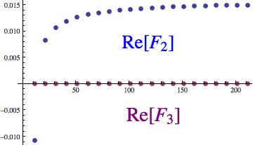
| (4.286) |
in contradistinction to the twisted ABJM case studied in (Benini et al., 2015a; Hosseini and Zaffaroni, 2016) but a priori expected from comparison with similar hermitian models (Marino, 2004; Mizoguchi, 2005). The dots in (4.286) represent terms without dependence on the magnetic fluxes . Specifically for and generic choice for there remains a universal contribution proportional to , as straightforward to infer out of (4.279) and (4.280).
5 Summary
The main scope of this work was to find an alternative path integral representation to justify the presence of the sum over fluxes in the topologically twisted index of (Benini and Zaffaroni, 2015) upon integration over real fields and without sacrificing positive definiteness of the bosonic part of the localising action.
An important point we stress upon, is that on the real path, the space of zero locus solutions of the localising term used in (Benini and Zaffaroni, 2015) is defined by the Bogomolnyi equations. On the set of smooth solutions to these equations is given by the set of flat connections on –which is trivial – and constant values for and . In approaching the problem with the same supercharge all along –namely following the approach that we have called VP-I–, one needs to exclude a point out of the in order to consider solutions with fluxes on , or equivalently, to consider real BPS vacua which are singular on . In the latter case, we have checked that the expression for the 3D TT Index of (Benini and Zaffaroni, 2015) is recovered after integration over the real path of fields by following the usual localisation method and without the need to sacrifice positive definiteness of the bosonic part of the action. We have shown the mechanism behind making these singular solutions part of the vanishing locus of the corresponding positive definite localising terms – on the "real" path (as explained in the introduction)–.
Following the same line of reasoning, we constructed and integrated out the localising term with positive definite bosonic part along the complex path of integration, reproducing in alternative manner the result of (Benini and Zaffaroni, 2015).
We have found the TT Index on times an open segment by carefully managing total derivatives. We have checked that the 3D TT Index on of (Benini and Zaffaroni, 2015) can be factorised into two blocks: the partition functions of TT theory on and TT theory on , respectively, upon localisation of the variational problem VP-II. At the level of one loop determinants, the matching condition (2.126) must be enlarged with the selection of complementary sets of KK modes on and . We have dubbed such modes as even and odd for obvious reasons that were explained in subsection 3.1.
The selection of a glueing prescription among BPS vacua from one side to the other , is specified by the matching condition (2.126) and implies the identification of fluxes from one side to the other. The selection of sign in (3.260) corresponds to localising the variational problem VP-II – mentioned in the previous paragraph –, specifically to the matching conditions (2.126). Instead, the choice on (3.260) seems to be related to allowing ’t Hooft modified solutions of the Bogomolnyi equations. An interesting point to pursue in the future, could be to study the dual description of theories that allow more general ’t Hooft modified BPS vacua. The aforementioned generalisations, are deformations of the 3D TT index and it would be interesting to interpret the presence of such domain walls or ’t Hooft deformations in the holographic dual set up. It would be interesting to provide an interpretation of the latter generalisations, from the point of view of microstate counting or deformations of supersymmetric black holes (Benini et al., 2015a; Hosseini and Zaffaroni, 2016; Benini and Zaffaroni, 2016; Gnecchi et al., 2016). Those interesting lines of analysis will be pursued elsewhere.
Acknowledgments
The author thanks Francesco Benini for his comments and suggestions, Victor I. Giraldo Rivera and Lorenzo di Pietro for their careful reading and critics on a previous version of the manuscript and to Leopoldo A. Pando Zayas, Junya Yagi, M. Nouman Muteeb and Antonio Sciarappa for useful conversations at different stages of this work. Thanks a lot to an anonymous referee for critics and suggestions and to Massimo Porrati and Sameer Murthy for drawing my attention to a subtle and important point. A grateful acknowledgement to The Abdus Salam ICTP, scientific and administrative staffs, for their kind hospitality during a couple of months of work. The work of the author is supported by CONICET.
Appendix A Geometry and Conventions
In (Benini and Zaffaroni, 2015) it was proposed a formula for the partition function of a gauge theory with two supercharges , with the same R-charge, on
| (A.287) |
, and , and type A semi-topological twisting along . Namely with a background gauge potential
| (A.288) |
with being the torsionless spin connection of (A.287).
The supercharges and are parameterised by two killing spinors (KS) and with R-charge . The KS satisfy the following equations
| (A.289) |
where and are the Pauli matrices. Under (A.288) the solution to the KS equations are with a constant eigenspinor of , with eigenvalue respectively
| (A.290) |
We will represent flat and curved indices by numbers and greek letters respectively. Our convention for spinor bilinear are summarised in the following set of definitions
This is the same definition written down in equation A.2 of (Closset et al., 2013). By complex conjugation , we mean transconjugation on the gauge algebra representation. As already mentioned in the bulk of the manuscript, the transformation parameter spinors are commuting. Physical spinor fields are anti commuting, hence transformation parameter spinors and physical spinor fields commute. For self completeness we write down the following set of identities
| (A.294) |
As for the covariant derivatives
In due time, the spin connection shall be absorbed in the magnetic flux term by a redefinition of -charge. The difference between the effective -charge felt by a "spin up" and "down" chiral spinor, like for instance the one between the components of the gaugino and , will be .
The gauge field strength components
| (A.298) |
A.1 Gauge Multiplet
In this appendix in essence we will follow the early literature on the topic, specifically (Kapustin et al., 2010; Alday et al., 2013; Peeters, 2007). Let the covariant derivative on the gaugini be defined as
| (A.299) |
As mentioned before, the spin connection shall be absorbed in the magnetic flux term by a redefinition of -charge. The difference between the effective -charge felt by a "spin up" and "down" chiral spinor, like for instance the components of the gaugino and , will be .
In our conventions the ’s are the Pauli matrices are hermitian. Let us define the object
| (A.300) |
that will be part of the definition of localising term
| (A.301) |
We stress, that the must not be confused with the operation. In fact is very similar to (the difference being for complexified fields). The former is obtained from the latter by substituting , and in (A.300) by their complex conjugated , and .
We stress that the object defined in Subsection 2.1 and the one defined in this subsection are no the same; their difference is
| (A.302) |
This difference arises because in (2.20) we substitute and by and respectively. Meanwhile in (A.300) we substitute and by and respectivelyWe apologise for the abuse of notation.
From (A.302) we conclude that the difference between the exact terms
| (A.303) |
is again exact and not only closed. After continuing the computation of the bosonic and fermionic parts with (2.19) instead of (A.301) and by using the covariant form of the algebra (2.9), we arrive to the same result obtained in subsection 2.1, where after using (2.12) we obtained (2.21) and (2.1). Instead of reporting the previously mentioned computation, in this subsection we report the computation that follows from the use of (A.301). As a nice difference we will obtain a covariant localising term in contradistinction with the analog results (2.21) and (2.1). However, as shall be seen in a while, this new term is not positive definite under the reality conditions (2.15). Instead, it will be positive definite under the more orthodox reality conditions
| (A.304) |
In the results to come, the reader will find the killing vector , which is defined as
| (A.305) |
| (A.308) | |||||
| (A.309) |
The boundary term is congruent with the equivalent C.6 in (Drukker et al., 2014). In this case the localising action is
| (A.310) |
From (A.306) is straightforward to see that this localisation action vanishes evaluated at the configurations (1.4).
A.2 Matter multipets
Let the covariant derivatives be
| (A.311) |
where is a background flavour connection.
Let us split the orthodox localising Lagrangian for matter (2.37) into parts and , where
| (A.312) |
with
| (A.313) | |||||
| (A.314) | |||||
| (A.315) |
Expanding this localising terms, we get the following bosonic and fermionic terms
| (A.316) | |||||
| (A.317) |
| (A.318) | |||||
| (A.320) |
The second term in (A.316) and the first in (A.318) combine to give
| (A.321) |
after using
| (A.322) |
The and above, are the field strengths of the and flavour background connections respectively.
The third and fourth terms in (A.316) combine with the third term in (A.318) to give a total derivative
| (A.323) |
After adding up (A.316) and (A.318)
| (A.324) | |||||
After adding up (A.317) and ()
| (A.325) |
is the same as equation (2.17) of (Benini and Zaffaroni, 2015) up to total derivatives that can be immediately read out of (A.324) and (A.325).
| (A.326) |
A.3 The orthodox localising terms
For completeness of presentation in this section we post the orthodox localising terms for vector and matter multiplets. For the vector multiplet
| (A.327) |
After expanding this term one gets
| (A.328) | |||||
| (A.329) |
From (2.29) and (A.327) and after using the following identities
| (A.330) | |||||
| (A.331) |
one arrives to the expected result
| (A.332) |
In (A.331) it is used the fact is only charged under the dynamical gauge group. Namely neutral under and flavour symmetries. The orthodox localising term for matter is
| (A.333) |
After expanding this term one gets
| (A.334) |
From (2.34) and (A.333) and after use of the following identity
| (A.335) |
one gets the expected result
| (A.336) |
Appendix B 1-loop determinants and JK Contour
B.1 Zero locus analysis
To solve the zero locus equations (2.56) we have first to fix the gauge. We choose
| (B.337) |
with . From the Bianchi identity of it follows that , next we suppose the fields and are single valued on and thenceforth it follows that and are also single valued. From the condition in the previous equation it follows that
| (B.338) |
Equation (B.338) together with the second line in (2.56) and (B.337) gives
| (B.339) |
What we have not mentioned so far is the dependence on and of , and . Here we will assume the GNO condition
| (B.340) |
for the constant magnetic flux – for instance, the latter assumption guaranties invariance under large gauge transformations of the classical Chern-Simons contribution–. The in (B.340) stands for an arbitrary weight of the corresponding Lie algebra. The equation for in (B.340) is uniquely solved – under GNO conditions – for specific values of and (up to trivial gauge transformations) that will be defined below.
The only missing equation can be solved uniquely for (by demanding independence of on and ),
| (B.341) |
with , and in the Cartan sub algebra of , and
The gauge invariant classes of saddle points (B.340)-(B.341) can be parameterised by the following gauge potentials
| (B.342) |
were , and represent mutually commuting elements of the gauge algebra. As already said, we stress that the weight vector components of the generators are supposed to be GNO quantised – the weights of belong to the Co-root lattice–.
As for the matter multiplets, let the contour of integration for the fields , , and be (2.18). The -BPS configurations along the path (2.18) are given by (2.54). Notice that the condition holds independently of the reality condition on . We remark this fact, because later on it will be needed to turn on a complex flavour line along . The result of the zero locus analysis presented in this section still holds in that case.
We must also notice, that to make an arbitrary linear variation of the matter action (2.35)+(2.36) at the zero locus (2.83)+(2.54)
| (B.343) |
vanish, it is needed the scalar fields to be solutions of
| (B.344) |
Otherwise the zero locus (2.54) will not be stable.
However as we are going to integrate along the path (2.18) it follows that at the zero locus (2.54) the following conditions hold,
| (B.345) |
In fact (B.345) coincides with the -BPS conditions for and consequently, it is a solution of the EOM coming from (B.344). This is guarantied from the fact that for the reality conditions (2.18) and saturates for the BPS real configurations (2.54). In words, the unique solution (saddle point) to
| (B.346) |
along (2.18) is (2.54). In a generic path of integration this will not be case.
As in (Benini and Zaffaroni, 2015), we will avoid the zones in the Coulomb branch that allow for non trivial solutions to (2.54). From the integration on of the zero locus equations (2.54) and (B.345) follows
| (B.347) |
where by we mean the product associated to the gauge representation carried by and . If the non trivial components and do not share a common zero eigenvalue under the action the matter multiplet zero locus is
| (B.348) |
Condition (B.348) eliminates the quadratic mixing of matter and gauge fluctuations around saddle points. We consider gauge representations where (B.348) is the only solution to (B.347) at least for some region of values of the moduli and . For example, with and in the adjoint where stands for the commutator , clearly (B.348) does not hold as the only solution of (B.347). For other irreps (B.348) generically holds in some region of the moduli space .
B.2 Integrality condition on
We remind here the definition of Chevalley basis of a semi-simple Lie algebra of rank which is generated by the set of generators with commutation relations
| (B.349) |
where
| (B.350) |
are the components of the Cartan matrix of . The roots are . The remaining generators are generated by the adjoint actions
| , | (B.351) | ||||
| , | (B.352) |
The remaining structure constants can be derived out of (B.349). They are integers too.
The acting onto a state in a representation with eigenvalues under the action of , with will define a new state, with eigenvalues with respect to . In similar fashion the ’s acting onto the state will define a new state with eigenvalues of shifted from to . From this analysis and (B.350), one can conclude that highest weight representations (and their sums) will necessarily obey
| (B.353) |
for every weight , in the basis in which the algebra takes the form (B.349). This is, a highest weight will necessarily obey because their Dynkin labels are positive integers ( with 2020 20 This is because we have defined with identified, in this way, as the dual to the Cartan generator . can also be thought as a state with eigenvalues under . Each one of the states is a HW state of an irreducible representation, better known as fundamental. Specifically, they carry a ”spin ” representation of the whose Cartan generator is . In our conventions the weight vector (fundamental) of the state is simply . From this point on, we will abuse of to denote the weights (fundamental) of its dual state. by definition. Additionally, every weight in the HW representation is obtained out of by performing a multiple subtraction of the roots (). Thence from (B.350) it follows (B.353).
Finally we show a property that was used in the main body of the manuscript. Let be a generic element in the Cartan. We remind that for and mutually commuting elements of the algebra then
| (B.354) |
Thenceforth
| (B.355) |
and we conclude that any function is invariant under .
B.3 1-loop determinants on
In this subsection we first show that the quadratic expansion of the chiral multiplets unorthodox () localising term around the ()-locus that we have found in previous subsection, coincides with the quadratic expansion obtained in (Benini and Zaffaroni, 2015) (In their case, when the zero mode vanishes and supersymmetry gets restored). We consider in the case of and in the case of . Namely we will study both versions, the 3D and TT theories on . The result of using either or is the same in the end.
As shall be noticed below, the 1 loop determinant of a vector multiplet is periodic along the real direction of the moduli with periodicity (Our conventions can be found in appendix B.2). As for matter multiplets, the period is related to both gauge invariance and absence of parity anomaly. In fact, a matter multiplet in a complex representation will have, generically, a 1 loop contribution with a period of . Indistinctly, under a shift of in , or under a parity inversion , the one loop contribution of a mode with gauge weight , that is an integer power of , changes by a factor of to that same power. That minus sign could survive in specific representations and in that case, the consequence of its presence is two-folded: 1-loop gauge and parity anomaly.
There are various ways to ensure the absence of the aforementioned gauge/parity anomaly out 2222 22 A sufficient condition without the use of Chern-Simons terms can be found in (Hori and Romo, 2013). We can also solve the gauge/parity anomaly by the use of Chern-Simons terms, however we don’t want to impose any constraint on the Chern-Simons content of the theory and consequently we must constraint the gauge representation carried by the matter content.. One possible solution is to consider matter multiplets in real representations. Another possibility would be to consider more than one matter multiplet in such a way their anomalies cancel each other out. One such example comes from considering two matter multiplets in complex conjugated representations of the gauge group in question. As shall be explicitly seen in the case of gauge group the product of the fundamental and antifundamental matter multiplets’ 1 loop factors becomes instead of periodic. Finally, we also elaborate about an issue pointed out in (Benini and Zaffaroni, 2015), the possible presence of "boundary contributions" and their geometrical meaning.
Let us start by the matter multiplet. The bosonic and fermionic parts of the action for quadratic fluctuations coming from (2.35) (after trivial integration by parts) and from (2.36), are
| (B.356) | |||||
| (B.357) |
with
| (B.362) |
In contradistinction with the operators coming out of (A.324) and (A.325)2323 23 This is, by discarding in those equations total derivatives. that for the zero locus we are considering provide non trivial contributions. , found after working with the form of the algebra (2.1), these operators do not look like the analog ones in (Benini and Zaffaroni, 2015). However as we shall see next, when evaluated on their corresponding zero loci, they will be the same. The term in (B.362) provides the contribution that in the approach followed by (Benini and Zaffaroni, 2015), comes from the non trivial (complex) saddle value of the auxiliary field that we have written in (1.3). Specifically, from the quadratic term proportional to in (A.324). When evaluated in their corresponding supersymmetric zero loci, the operators (B.362) are the same as the analog ones in (Benini and Zaffaroni, 2015) and thenceforth is straightforward to check that the final result for the 1-loop determinant is the same after changing by
| (B.363) |
with . Where is a representation of the gauge algebra. In subsection 3.1 we have computed this one loop contribution for . The computation is completely analog in this case. See appendix A.3 in (Benini and Zaffaroni, 2015) for other approaches to derive (B.363).
Now let us show that in the Chevalley basis (See appendix B.349) and for non gauge/parity anomalous gauge representations, or as supposed in this work, representations that remain invariant under the inversion , the 1 loop determinant for the chiral multiplet is invariant under the transformation . An important property to keep in mind is that
| (B.364) |
were is any of the Cartan generators. In arriving to (B.364) we have used the property , that comes from the fact that the scalar product between the weights in a given representation and the fundamental weights of the algebra obeys the integrality condition , that we have elaborated upon in appendix B.2. From (B.364) and it follows that if representation is invariant under then
| (B.365) |
and consequently
| (B.366) |
Similarly from (B.364) and is immediate to prove that where by and we mean the one loop contributions of a couple of chiral multiplets with coincident quantum numbers but with complex conjugated gauge representations and .
While analysing the JK procedure and the potential presence of the so called "boundary contributions", we will find useful to know about the asymptotic behaviour in the limit . Also, as we shall see next, this asymptotic behaviour for involves only through the constant phase . As already argued when we use a complex representation for the matter sector we should also add up a complementary matter multiplet in the complex conjugated representation with the same additional charges (R-charge, etc). So, to illustrate clearly, we start by writing down a particular example of (B.363) for matter in the fundamental and anti-fundamental of
| (B.367) |
where and , are a flavour complex Wilson line along and flux onto , respectively. Notice that for with the asymptotic expansion of the product
| (B.368) |
will only depend on through the phase that can be absorbed with the topological holonomy (2.62). Thence, as the integrand will be independent on and blindly following the argument given in section 2.3.4 of (Benini and Zaffaroni, 2015) if we will simply ignore the presence of "boundary contributions". To the reader which is not familiar with this terminology, it shall be seen in a while what is meant by "boundary contributions". Notice that it does not matter whether one takes the plus or minus sign in the limit, the asymptotic behaviour (B.368) will not approach zero.
Next, we move on to the study the 1 loop contribution of the vector multiplet. We expand the localising term (2.21), around the zero locus (B.342) to get
where in this section .
In (B.3) we have integrated by parts , and . This discarded total derivative vanishes because we are considering (D,D) boundary conditions for the vector multiplet in order to annihilate the supersymmetric variation of the modified Chern-Simons terms.
The BRST term is
| (B.386) |
and the non “covariant" BRST transformations are
| (B.387) |
After imposing the gauge fixing condition
| (B.388) |
the quadratic expansion for bosonic density of Lagrangian is
| (B.389) |
where
| (B.390) | |||||
| (B.391) |
The basis of functions on to use in this case will be
| (B.392) |
with
| (B.393) |
The and grow at step 1. We consider the roots to be outside of the Cartan sub algebra values, in order not to get a vanishing determinant. The above are the spin spherical harmonics (See (Wu and Yang, 1976; Benini and Cremonesi, 2015; Doroud et al., 2013)). The magnetic levels in (B.392) are selected from demanding consistency with supersymmetry, as we shall explain in a while.
After the change of variables on each patch
| (B.394) |
the functional integration over (notice this change of variable has unit Jacobian) gives
| (B.395) |
The operator is invertible provided
| (B.396) |
If (B.396) holds then (B.395) is finite. Condition (B.396) kills the zero modes of and implies the elimination of the Cartan roots (weights) .
The contribution (B.395) cancels out the functional integration of , the Fadeev-Popov determinant, which equals , over the same functional space. Finally, we integrate over the functional space in to get
| (B.397) |
The quadratic density Lagrangian for the gaugino fluctuations was written in (B.3). Notice that the off diagonal operator does not affect the value of the determinant to compute. In this sense, the use of the non covariant localising term (2.19) and (2.67) simplifies the job of computing one loop determinants. One must compute the determinants on by expanding the space of functions on spanned by the following basis of functions
| (B.398) |
and
| (B.399) |
The relative magnetic levels are obtained from consistency with the supersymmetry transformations (2.11) and (2.66). Specifically from their term after expanding with (2.115) one gets
| (B.400) |
From the equations in the first and third lines we can infer that the magnetic levels of and must coincide with the ones of and . From the second line we conclude that , and have coincident magnetic level. A similar analysis with the BRST transformation shows that and must have the same magnetic level as which must be the same as . After analysing the terms in the expansion of algebras one concludes that the magnetic levels are the ones written in (B.392) and (B.398).
After functional integration of the quadratic localising action of the gaugino and antigaugino linear fluctuations one gets the factors
| (B.401) |
whose product with (B.397) simplifies to
| (B.402) | |||||
Where is the set of roots and is the Weyl vector (). The arbitrary regularisation constant for the vector multiplet is defined to be for convenience. Finally, we obtain the known answer
| (B.403) |
B.4 Vector multiplet 1- loop determinant in the complex path of integration
The quadratic actions coming out of the localising terms (2.135) and (2.136), along the complex path (2.132) and after gauge fixing condition (B.388) is imposed, are
| (B.404) | |||||
| (B.405) |
where
| (B.406) |
The integrates trivially. The integration of and gives after following the same steps outlined in the previous subsection
| (B.407) |
The integration of and , multiplied by the integration of and following from the BRST action (B.386) gives
| (B.408) |
As already mentioned, we will not integrate over the zero modes and in order not to obtain vanishing results. The product of the two contributions (B.408) and (B.407), was already shown in the previous subsection to be (B.403), hence concluding our analysis of the complex path of integration used in (Benini and Zaffaroni, 2015). The analysis and results of the one loop contribution of the matter and Chern-Simons terms in the complex path, are equivalent to the analysis and results that were already presented for the real path of integration, so we do not repeat them.
B.5 A Jeffrey Kirwan Contour
One possible choice of segment of integration for the moduli is
| (B.409) |
From the usual Jeffrey Kirwan (JK) perspective, the selection of the chamber (B.409) is analog to the selection of a reference vector with components . Integration over the set of contours (B.409) can be mapped to the computation of residues generated by a set of charges (weights) .
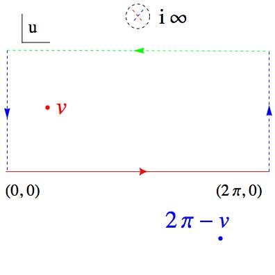
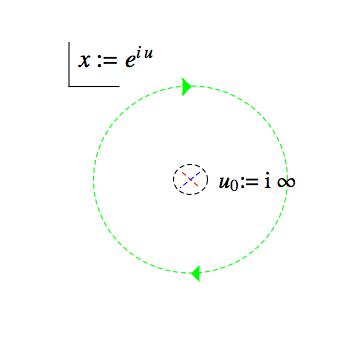
We say that the set of charges , with , generate a residue around a point if the integrand of the partition function looks like
| (B.410) |
in a vicinity of , with and such that
| (B.411) |
Condition (B.411) is necessary to have a non trivial integration form (B.410). It is not sufficient because could "accidentally" vanish. Each one of the , is a vector of elements. By , in (B.411), we mean the determinant of the matrix whose columns (or raws) are the vectors with .
The Jeffrey Kirwan recipe amounts to select residues generated by provided
| (B.412) |
In words, condition (B.412) selects residues coming from poles associated to positively charged chiral (). This is, iff then . The reference vector must not belong to the boundary of the Cone.
Let us see for the case of rank one gauge group how the selection of segment (B.409) can be identified with the JK procedure just reviewed. For that we define the auxiliary closed contour composed by the union of (B.409) and
| (B.413) | |||||
| (B.414) | |||||
| (B.415) |
In the sake of clarity of presentation we have depicted this closed contour in figure 3 to the left. If the integrand of (3.267) is - periodic, integration over the segments and cancel out 2525 25 They run in opposite direction. and
| (B.416) |
From (B.416) and taking the limit we conclude that
| (B.417) | |||||
| (B.418) |
where by we mean the sum of residues on the upper half plane but discarding the potential "boundary contribution" (as called in (Benini and Zaffaroni, 2015))
| (B.419) |
This contribution can be computed by performing the exponential map . In this way the line , the green line in figure 3, is mapped to a circumference centred at . Consequently equates to the residue of the integrand in the new coordinates , at .
Before moving on, let us comment about the relation between our procedure of integration and the JK prescription given in (Benini and Zaffaroni, 2015). Each factor in the matter one loop determinant (B.363) has a pole at provided . After turning on the complex flavour lines with and the poles coming from positive (negative) charges which originally are sitting at get shifted to () which is in the upper (lower) half complex plane , and hence enclosed (excluded) by . Namely our selection of encloses the poles associated to positive charges . This is the same result one gets by applying the JK prescription with . The other choice corresponds to close the segment (B.409) over lower half of the complex plane. We will not treat the case of higher rank gauge groups, in any deepness, but the graphical analysis can be generalised to that case.
References
- Benini and Zaffaroni (2015) F. Benini and A. Zaffaroni, JHEP 07, 127 (2015), arXiv:1504.03698 [hep-th] .
- Benini et al. (2015a) F. Benini, K. Hristov, and A. Zaffaroni, (2015a), arXiv:1511.04085 [hep-th] .
- Hosseini and Zaffaroni (2016) S. M. Hosseini and A. Zaffaroni, (2016), arXiv:1604.03122 [hep-th] .
- Chung and Yoshida (2016) H.-J. Chung and Y. Yoshida, (2016), arXiv:1605.07165 [hep-th] .
- Nedelin et al. (2016) A. Nedelin, F. Nieri, and M. Zabzine, (2016), arXiv:1605.07029 [hep-th] .
- Strominger and Vafa (1996) A. Strominger and C. Vafa, Phys. Lett. B379, 99 (1996), arXiv:hep-th/9601029 [hep-th] .
- Sen (2008) A. Sen, JHEP 11, 075 (2008), arXiv:0805.0095 [hep-th] .
- Witten (1991) E. Witten, (1991), arXiv:hep-th/9112056 [hep-th] .
- Jeffrey and Kirwan (1993) L. C. Jeffrey and F. C. Kirwan, in eprint arXiv:alg-geom/9307001 (1993).
- Closset et al. (2015) C. Closset, S. Cremonesi, and D. S. Park, JHEP 06, 076 (2015), arXiv:1504.06308 [hep-th] .
- Honda and Yoshida (2015) M. Honda and Y. Yoshida, (2015), arXiv:1504.04355 [hep-th] .
- Closset and Kim (2016) C. Closset and H. Kim, (2016), arXiv:1605.06531 [hep-th] .
- Pestun (2012) V. Pestun, Commun. Math. Phys. 313, 71 (2012), arXiv:0712.2824 [hep-th] .
- Benini et al. (2014) F. Benini, R. Eager, K. Hori, and Y. Tachikawa, Lett. Math. Phys. 104, 465 (2014), arXiv:1305.0533 [hep-th] .
- Benini et al. (2015b) F. Benini, R. Eager, K. Hori, and Y. Tachikawa, Commun. Math. Phys. 333, 1241 (2015b), arXiv:1308.4896 [hep-th] . CITATION = ARXIV:1308.4896;
- Imamura and Yokoyama (2011) Y. Imamura and S. Yokoyama, JHEP 04, 007 (2011), arXiv:1101.0557 [hep-th] .
- Borokhov (2004) V. Borokhov, JHEP 03, 008 (2004), arXiv:hep-th/0310254 [hep-th] .
- Cremonesi (2015) S. Cremonesi, J. Phys. A48, 455401 (2015), arXiv:1505.02409 [hep-th] .
- Pasquetti (2012) S. Pasquetti, JHEP 04, 120 (2012), arXiv:1111.6905 [hep-th] .
- Beem et al. (2014) C. Beem, T. Dimofte, and S. Pasquetti, JHEP 12, 177 (2014), arXiv:1211.1986 [hep-th] .
- Gadde et al. (2015) A. Gadde, S. S. Razamat, and B. Willett, JHEP 11, 163 (2015), arXiv:1506.08795 [hep-th] .
- Redlich (1984a) A. N. Redlich, Phys. Rev. Lett. 52, 18 (1984a).
- Redlich (1984b) A. N. Redlich, Phys. Rev. D29, 2366 (1984b).
- Kapustin and Witten (2007) A. Kapustin and E. Witten, Commun. Num. Theor. Phys. 1, 1 (2007), arXiv:hep-th/0604151 [hep-th] .
- Yoshida and Sugiyama (2014) Y. Yoshida and K. Sugiyama, (2014), arXiv:1409.6713 [hep-th] .
- Suzuki (2012) M. Suzuki, ArXiv e-prints (2012), arXiv:1211.2953 [math.CA] .
- Marino (2004) M. Marino (2004) arXiv:hep-th/0410165 [hep-th] .
- Mizoguchi (2005) S. Mizoguchi, Nucl. Phys. B716, 462 (2005), arXiv:hep-th/0411049 [hep-th] .
- Benini and Zaffaroni (2016) F. Benini and A. Zaffaroni, (2016), arXiv:1605.06120 [hep-th] .
- Gnecchi et al. (2016) A. Gnecchi, U. Gursoy, O. Papadoulaki, and C. Toldo, (2016), arXiv:1604.04221 [hep-th] .
- Closset et al. (2013) C. Closset, T. T. Dumitrescu, G. Festuccia, and Z. Komargodski, JHEP 05, 017 (2013), arXiv:1212.3388 [hep-th] .
- Kapustin et al. (2010) A. Kapustin, B. Willett, and I. Yaakov, JHEP 03, 089 (2010), arXiv:0909.4559 [hep-th] .
- Alday et al. (2013) L. F. Alday, D. Martelli, P. Richmond, and J. Sparks, JHEP 10, 095 (2013), arXiv:1307.6848 [hep-th] .
- Peeters (2007) K. Peeters, (2007), arXiv:hep-th/0701238 [HEP-TH] .
- Drukker et al. (2014) N. Drukker, T. Okuda, and F. Passerini, JHEP 07, 137 (2014), arXiv:1211.3409 [hep-th] .
- Hori and Romo (2013) K. Hori and M. Romo, (2013), arXiv:1308.2438 [hep-th] .
- Wu and Yang (1976) T. T. Wu and C. N. Yang, Nucl. Phys. B107, 365 (1976).
- Benini and Cremonesi (2015) F. Benini and S. Cremonesi, Commun. Math. Phys. 334, 1483 (2015), arXiv:1206.2356 [hep-th] .
- Doroud et al. (2013) N. Doroud, J. Gomis, B. Le Floch, and S. Lee, JHEP 05, 093 (2013), arXiv:1206.2606 [hep-th] .