IFIC/16-42
Unifying leptogenesis, dark matter and high-energy neutrinos with right-handed neutrino mixing via Higgs portal
Abstract
We revisit a model in which neutrino masses and mixing are described by a two right-handed (RH) neutrino seesaw scenario, implying a strictly hierarchical light neutrino spectrum. A third decoupled RH neutrino, with mass , plays the role of cold dark matter (DM) and is produced by the mixing with a source RH neutrino, with mass , induced by Higgs portal interactions. The same interactions are also responsible for decays. We discuss in detail the constraints coming from DM abundance and stability conditions showing that in the hierarchical case, for , there is an allowed window, , necessarily implying a contribution, from DM decays, to the high-energy neutrino flux recently detected by IceCube. We also show how the decays of the two coupled RH neutrinos can explain the matter-antimatter asymmetry of the universe via leptogenesis in the quasi-degenerate limit. In this case, the DM mass should be within a tighter range 300 GeV 300 TeV. We discuss the specific properties of this high-energy neutrino flux and show the predicted event spectrum for two exemplary cases. Although DM decays, with a relatively hard spectrum, cannot account for all the IceCube high-energy data, we illustrate how this extra source of high-energy neutrinos could reasonably explain some potential features in the observed spectrum. In this way, this represents a unified scenario for leptogenesis and DM that could be tested during the next years with more high-energy neutrino events.
1 Introduction
The possibility of explaining the dark matter (DM) and baryon asymmetry of the universe within a unified picture is an attractive idea, intensively explored during recent years [1]. This is also motivated by the simple observation that baryons and DM give a similar contribution to the cosmic energy budget.
Moreover, since both DM and baryon asymmetry of the universe require new physics, it is conceivable that they should be ultimately explained within a common model. An extension of the standard model (SM) is also required by neutrino masses and mixing established by neutrino oscillation experiments and, therefore, it is quite natural to look at neutrino physics as a possible source for cosmological DM and matter-antimatter asymmetry.11 1 Curiously within errors one has , where and are the atmospheric and solar neutrino mass scales, respectively. The simplest way to describe neutrino masses and mixing is by adding to the SM Lagrangian right-handed (RH) neutrino Yukawa couplings and a Majorana mass term. In the seesaw limit one obtains the seesaw formula for the low-energy neutrino mass, nicely explaining why left-handed (LH) neutrinos are much lighter compared to all other massive fermions [2].
It is then natural to think whether heavy RH neutrinos can play a cosmological role. In the traditional high-energy scale leptogenesis scenario [3], RH neutrino decays are the source of the observed baryon asymmetry. In the MSM scenario [4], the lightest RH neutrino with (keV) mass can play the role of DM, with the correct abundance produced by active-sterile neutrino mixing. At the same time, the mixing between the two heavier RH neutrinos can also produce the observed baryon asymmetry [5]. In this model, however, the neutrino Yukawa couplings are many orders of magnitude smaller than those of all other particles and somehow the original motivation of the seesaw is not addressed.22 2 However, in Ref. [6] it was shown how the specific MSM neutrino Yukawa matrix could arise as a consequence of a lepton number symmetry slightly broken by the Majorana mass terms and Yukawa coupling constants. For more details on the MSM model we refer the reader to Ref. [7].
As a remedy, it was proposed [8] that if one of the RH neutrinos decouples and it is stable on cosmological time scales, it could play the role of DM and the same mixing among RH neutrinos could also reproduce the correct DM abundance. This is possible if one introduces a non-renormalizable operator , a simple example of Higgs portal models [9], arising from new physics at some scale with additional couplings . The presence of this new interaction would enhance medium effects opening a new production mechanism from RH-RH neutrino mixing (occurring much above the electroweak scale) rather than from RH-LH neutrino mixing (occurring much below the electroweak scale), as in the MSM. At the same time it would also be responsible for the DM RH neutrino, with mass , eventually to decay, producing high-energy neutrinos33 3 For limits on DM decays with neutrino detectors, see Refs. [10, 11, 12, 13]. and it was pointed out44 4 In Ref. [8] it was noticed that a possible explanation of the PAMELA excess would also imply a potential signal at the IceCube detector. that this flux could be detectable at neutrino telescopes such as IceCube [8].
Intriguingly, the IceCube detector has recently detected the first ever high-energy neutrino events of extraterrestrial origin [14, 15], i.e., that cannot be accounted for by the known atmospheric neutrino flux. The energies of these events are as high as , i.e., within the natural range of masses needed by the mechanism of cold DM from RH neutrino mixing, as we will discuss in detail. Indeed, very heavy DM decays have been proposed to account for part or all of these events [16, 17] and different constraints, within different models, have been presented [18, 19, 20, 21, 22, 23, 24, 25, 26, 27, 28, 29], showing that this could be a potential explanation of the observed events (or part of them). Encouraged by this phenomenological picture, in this paper we revisit the cold DM RH neutrino mixing scenario discussing a few important aspects and showing how to test it with high-energy neutrino detectors such as IceCube and also showing explicitly how the same set up can accommodate the matter-antimatter asymmetry of the universe via leptogenesis, as first pointed out55 5 A cosmologically stable RH neutrino playing the role of DM has also been proposed within left-right symmetric models [30], also in combination with leptogenesis [31], and within a hybrid seesaw model [32]. in Refs. [8, 33, 34].
The paper is organised as follows. In Section 2 we review the idea of the seesaw mechanism with one decoupled RH neutrino and the cold DM RH neutrino mixing scenario. In particular we discuss in detail how in the simplest scenario, in order to reproduce the correct DM abundance with a cosmologically stable candidate, has to be in the range GeV– EeV in the hierarchical case, for . We also discuss a few ingredients, some of which represent quite plausible possibilities, that might relax the constraints especially in the quasi-degenerate limit with . In Section 3 we show how the observed matter-antimatter asymmetry can be explained in this model via leptogenesis and in this case the range for restricts to TeV–10 PeV intriguingly overlapping with the range of neutrino energies detected at IceCube. In Section 4 we discuss the features of the predicted high-energy neutrino flux and its related event spectrum in the IceCube detector, for two exemplary cases for which the DM mass is above a few 100 TeV. We compare these results with the observed event spectrum and show that, although a DM-only signal cannot explain the 4-year IceCube spectrum, it could help to explain some of its features. Finally, in Section 5 we draw our conclusions.
2 The cold DM RH neutrino mixing scenario
In this section, we revisit the DM RH neutrino scenario [8], combine all constraints using the most recent data and we finally discuss some plausible viable scenarios and the allowed range of values for . In particular we show that relaxing the assumption of ultra-relativistic thermal abundance at the resonance, the hierarchical case () becomes viable extending the range of allowed values for .
2.1 From the minimal seesaw Lagrangian to Higgs portal interactions
We assume the usual minimal SM extension with three RH neutrinos with Yukawa couplings and a Majorana mass matrix . After spontaneous symmetry breaking, the Higgs vacuum expectation value (vev) generates a neutrino Dirac mass so that the neutrino mass terms can be written as ()
| (1) |
where with , in a basis where the Majorana and charged lepton mass matrices are diagonal. In the seesaw limit, , the set of neutrino masses splits into a light neutrino set with masses given by the seesaw formula
| (2) |
where is the leptonic mixing matrix and for the light neutrino masses we adopt the convention . From neutrino oscillation experiment global analyses we know that [35, 36] , where for normal ordering (NO) and for inverted ordering (IO), and for NO and for IO, where .
We parameterise the mixing matrix in the usual way for NO,
| (3) |
where , , is the Dirac phase and and are the two Majorana phases. For IO, since we use the convention , this has to be cyclically permuted such that
| (4) |
The best fit values and () confidence level (C.L.) ranges of the reactor, solar and atmospheric mixing angles for NO (left column) and IO (right column), are given by [35, 36]
| (5) |
where the LID method of the NOA -appearance data has been considered. In addition, current experimental data also start to set constraints on the Dirac phase and the best fit values and C.L. intervals are found to be, for NO and IO respectively,
| (6) |
though all values are still allowed at C.L. for NO and for IO. On the other hand, although the best fit in this analysis is obtained for IO, none of the two orderings is clearly favoured over the other (using different methods gives rise to different results in this respect [35, 36]).
We assume that one of the three RH neutrinos, , has Yukawa couplings small enough to guarantee its stability on cosmological time scales so that it is a potential DM candidate [8]. In this case, necessarily, the neutrino Dirac mass matrix has to be written in one of the three following forms,
| (7) |
corresponding effectively to a two-RH neutrino model in which either the lightest RH neutrino , the next-to-lightest or the heaviest is decoupled and has to be identified with .66 6 These special forms can be easily justified imposing for example a symmetry under which is odd and the other two RH neutrinos are even. The same forms have also been considered in a different context in order to have resonant leptogenesis testable at colliders [37]. These three forms for , with three texture zeros, can be parameterised in terms of nine physical parameters, since three phases can be always reabsorbed in the LH neutrino fields. In the Yukawa basis the Dirac mass matrix is diagonal and we can express it as , with . The transformation from the basis where the charged lepton and Majorana mass matrices are diagonal to the Yukawa basis can be described in terms of two unitary matrices, and , acting respectively on the LH and on the RH neutrinos, explicitly
| (8) |
Our working assumption, Eq. (7), necessarily implies and consequently, from the seesaw formula, Eq. (2), one has : in our scenario light neutrinos are strictly hierarchical, either normal hierarchy (NH) or inverted hierarchy (IH). The matrix is the RH neutrino mixing matrix and connects the Yukawa eigenstates to the mass eigenstates : (). It can be regarded as the analogue of the leptonic mixing matrix for the light neutrinos and it can be similarly parameterised by three mixing angles and three phases. If , then is strictly stable and it coincides exactly with , implying that the two mixing angles of with the other two RH neutrinos vanish.
We can also conveniently express in the orthogonal parameterisation [38],
| (9) |
where is the orthogonal matrix encoding information on the RH neutrino total decay widths and total asymmetries. The three forms for in Eq. (7) necessarily imply, respectively, the three following forms for :
| (10) |
where is a complex angle and is a discrete parameter and the two possible values correspond to two different distinct branches of , with positive and negative determinant respectively [39]. Notice that the nine (real) parameters needed to parameterise the Dirac mass matrix are in this case given by five parameters in the leptonic mixing matrix (three mixing angles, one Dirac phase, one Majorana phase), two LH neutrino masses, and , and finally two real parameters in the complex mixing angle .
If Eq. (7) is assumed to hold exactly, then would be strictly stable. However, in this case could not be produced by any interaction, except maybe via gravitational ones, for example at the end of inflation, if it has a mass close to the inflaton mass [40]. In that case, would likely be identified with the heaviest RH neutrino, . At the same time, it would be questionable whether such a particle would exist at all, not having any interaction. One could think of solving both problems by perturbing the form Eq. (7) for the Dirac mass matrix, introducing some tiny Yukawa coupling . In this case would decay with a lifetime (after EW symmetry breaking)
| (11) |
From the latest IceCube results, as we will discuss in detail, one has to require , so that the DM Yukawa coupling would be
| (12) |
which is too tiny to think of any DM production mechanism via Yukawa interactions. One possible solution, the so called MSM model [4], is to have the lightest RH neutrino sufficiently light to dominantly decay into three ordinary neutrinos, in a way that . At the same time, in this way the LH-RH neutrino mixing angle is enhanced and this would induce a sizeable RH neutrino production from mixing. The conditions for the cosmological stability and the correct DM abundance can then be satisfied for a mass of the lightest RH neutrino in the keV range.
However, this solution has the disadvantage of a drastic suppression of all three Yukawa couplings compared to those of all other massive fermions. An alternative possibility is to produce , not necessarily the lightest, through the mixing with the other (two) thermalised RH neutrinos [8]. However, in this case it is easy to see that the mixing cannot be the minimal mixing encoded in the matrix, defined by Eq. (8), which describes the mismatch between the Yukawa basis and the basis where the RH neutrino mass matrix is diagonal. This is so since the mixing angles of with the other two RH neutrinos would be (), too tiny to produce a sizeable abundance, as . For all practical purposes, we can then neglect such small mixing angles and consider .
A way out is to introduce non-standard RH neutrino interactions originating from new physics at an effective scale . At lower energies, this gives rise to a non-renormalizable effective operator, an example of Higgs portal interactions [9], which in the Yukawa basis can be written as77 7 Here, we do not refer to any specific model generating this interaction and, therefore, we will treat as a free phenomenological parameter. Below, we will give an example of a simple model able to justify the large values of that we will obtain. () [33, 8, 41]
| (13) |
Let us show that when introducing this new non-standard interaction, the RH neutrino mixing can lead to the correct abundance.
2.2 Estimation of the abundance
In general, the new interaction couplings are non-diagonal in the Yukawa basis and this can provide an efficient source for the RH neutrino mixing. Indeed they would give a contribution to the effective matter potential of the RH neutrino, which in the Yukawa basis is given by [8]
| (14) |
On the other hand, the Yukawa interactions clearly produce a diagonal contribution to the RH neutrino Hamiltonian in the Yukawa basis given by [42]
| (15) |
where is the energy and RH neutrinos are assumed to be in ultra-relativistic thermal equilibrium (of course, this is not true for , since in this case ). In the mass eigenstates basis one also has the usual kinetic contribution.
Let us assume that the mass eigenstate corresponding to mixes with just one of the other two thermalised (mass eigenstate) RH neutrinos. This would play the role of the source RH neutrino, that we refer to as , and which is in general a linear combination of and .
In this way, we have a simple two-neutrino mixing formalism, neglecting for the time being the mixing with the third RH neutrino mass eigenstate (the interfering RH neutrino). We will comment on this at the end of this section, showing that indeed the mixing with this RH neutrino can be neglected, since only the mixing with one RH neutrino can satisfy simultaneously all constraints. However, in Section 3 we will see that plays a crucial role for leptogenesis (and of course, it is in any case necessary in order to reproduce correctly the neutrino oscillation experimental data).
The source RH neutrino has a Yukawa coupling where is the index corresponding to the mass eigenstate coinciding with . If we introduce the effective neutrino mass and parametrise it as , then we can write88 8 For example, if we again consider the third form for in Eq. (7) corresponding to the third form for in Eq. (10) and identify with , then the effective neutrino mass can be expressed in terms of as (16) Clearly, one has , corresponding to . There is no upper bound for but values correspond to , necessarily implying a fine-tuning in the seesaw formula at the level of .
| (17) |
In this way, following the standard procedure, we can write the Hamiltonian for the mixed RH neutrinos in the mass eigenstate basis as
| (18) |
where we defined and we (reasonably) assumed that non-standard interactions are much smaller than Yukawa interactions, such that within the relevant temperature range (see below). In the ultra-relativistic limit we can then write and . As usual, subtracting a contribution to proportional to the identity that does not contribute to the mixing, we are left with the effective mixing Hamiltonian
| (19) |
where we defined . If we now describe the neutrino spectrum by its average momentum, , and introduce the dimensionless effective potential and the effective mixing angle , due to the presence of the non-standard interactions, we can recast as
| (20) |
The energy eigenstates in matter have energies and . While the temperature drops down, these tend to get closer to the mass eigenstates and and
| (21) |
The mixing angle is given by
| (22) |
Notice that also the mixing angle in vacuum is a function of the temperature. If , equivalent to having , there is a resonance for . This resonance condition is verified for a specific value of the temperature:
| (23) |
It is also useful to introduce the quantity
| (24) |
showing that for a fixed and decreasing , then decreases (i.e. increases). This observation will be useful when we will discuss the hierarchical case .
At , the coupled RH neutrino , the interaction eigenstate, is assumed in thermal ultra-relativistic equilibrium (later on we will see that a lower value of the abundance is also possible and even preferred) and this basically coincides with the matter eigenstate with energy . Since the process is highly non-adiabatic, does not track the matter eigenstate while the temperature drops down. In this way, at , just a small fraction of is converted non-adiabatically into the DM RH neutrinos, , the interaction eigenstate that in the absence of mixing would coincide with the mass eigenstate . Let us stress that even after spontaneous symmetry breaking, at zero temperature, there is still a tiny non vanishing mixing angle, , such that (the genuine DM state) does not exactly coincide with but also has a tiny component, which is one of the reasons why it is not strictly stable as we will see. The fraction of converted into can be calculated using the Landau-Zener formula99 9 See Ref. [33] for a derivation within the density matrix formalism.
| (25) |
where is the adiabaticity parameter at the resonance, defined as (see, e.g., Ref. [43])
| (26) |
Then, a straightforward calculation gives first
| (27) |
| (28) |
and then, using , we finally find1010 10 Here we correct the factor in the denominator given in Ref. [8], that was instead of .
| (29) |
where is the expansion rate at the resonance and is the number of degrees of freedom at the resonance. This can be assumed to have approximately the SM value plus the contribution from the , so that . In this way we obtain
| (30) |
For the DM abundance one obtains the simple relation
| (31) |
where is the DM-to-photon number ratio at the end of resonant conversion. Since we are assuming that at the resonance the ’s are fully thermalised, then and, using Eq. (25), one obtains
| (32) |
From Eq. (24), we can express in terms of ,
| (33) |
Plugging this expression into Eq. (30) and re-expressing in terms of , we find
| (34) |
In the quasi-degenerate limit, the ratio is simply . The assumption that is in ultra-relativistic thermal equilibrium at the resonance imposes both a lower bound and an upper bound on . The condition that they are ultra-relativistic simply requires , since for larger values, the abundance is Boltzmann suppressed.
There is also a less trivial lower bound. In our setup, the only interactions that can thermalise are the Yukawa couplings. Assuming that after inflation the abundance is negligible1111 11 This is a logical self-consistency condition: if we postulate that some external mechanism produces some amount of , then the same external mechanism could be invoked to produce also . A possibility is that, at the end of inflation, the inflaton field does not couple to but only to and in this case, one could even assume an abundance above the thermal value. We will be back to this point at the end of this section. then would thermalise at , defined as that value of such that for initially vanishing abundance. Since we are assuming ultra-relativistic thermal equilibrium, then we have to impose .
Inverse decays would thermalise at [44], where . However, when scatterings involving top quarks and gauge bosons are also taken into account, the thermalisation is more efficient and , valid for . Further analyses have included more processes and finite temperature effects, such as thermal masses, typically enhancing RH neutrino production and thus, going in the direction of yielding smaller values of [46]. The latest analysis, employing a closed path formalism [47], finds for the total production rate , which is equivalent to , and implies . Notice that, in principle, , and consequently , can be made arbitrarily small by making arbitrarily large, but a value , corresponding to , necessarily involves some amount of fine-tuning in the seesaw formula. In any case, it is convenient to treat, for the time being, as a free parameter since it plays a crucial role. Moreover, when we will discuss the case of dynamical abundance at the resonance, we will show that it is possible to have arbitrarily small values of , although below .
Plugging now the expression for , Eq. (34), into the DM abundance, Eq. (32), one obtains
| (35) |
Latest Planck satellite results find for the DM abundance (combining temperature and polarization anisotropies and gravitational lensing) [48],
| (36) |
This implies that the correct value of to reproduce the observed DM abundance is given by
| (37) |
showing that the mechanism can reproduce the correct DM abundance for reasonable values of .1212 12 One has values GeV. If , quite small couplings are required. However, even if one imposes , it is not difficult to build models with an effective scale of energy . For example in GUT theories the RH neutrinos can couple, with a small Yukawa coupling , to a heavy scalar with mass and this via an one-dimensional trilinear coupling to the SM Higgs via a tadpole graph. In this case, integrating out the heavy scalar, one obtains [34].
In the hierarchical case, . If is set to , then . These values imply unacceptably high values of the reheat temperature, since it is required at the end of inflation. This was the argument used in [8] to rule out the hierarchical case. However, as we said, we will show that values are actually possible if the assumption of ultra-relativistic thermal abundance at the resonance is relaxed. Interestingly, in light of current IceCube high energy neutrino data, we will see that this will rescue the possibility to open a window for , without any additional non-minimal ingredient or resorting to theoretical uncertainties.
On the other hand, in the quasi-degenerate case, one has , so that we can write
| (38) |
This shows that, for a fixed value of and a sufficiently small value of , it is always possible to satisfy the condition for ultra-relativistic thermal equilibrium, .
We have now to worry whether the same new interactions responsible for the production of the abundance can spoil the DM stability on cosmological scales giving unacceptably short lifetimes with high-energy neutrino flux in disagreement with the IceCube data. Of course, at the same time, this instability also represents an opportunity to identify a potential observable contribution to the detected IceCube high-energy neutrinos, as first pointed out in Ref. [8]. This implies that the model has predictive power and can be tested.
2.3 DM decays
The decays can proceed through two dominant decay channels [8, 33, 34]. The first channel is due to the mixing itself that produces the observed DM abundance. Indeed, after electroweak spontaneous symmetry breaking, though the finite temperature-induced mixing is negligible, the operator in Eq. (13) still generates a mixing (in vacuum) between and with mixing angle1313 13 It is possible to derive this expression going through the usual lines already reviewed to derive .
| (39) |
where is the total decay width for GeV [50].
In this way, does not exactly coincide with the stable neutrino mass (and Yukawa) eigenstate , but has a tiny (fast-decaying) component that would decay quickly into gauge bosons and leptons. As we describe below, the flavour composition of the produced light neutrinos could play an interesting role in the analysis of the high-energy neutrino flux predicted by the mechanism. The decay rate for this process of DM decay via mixing is then simply given by [33, 34]
| (40) |
This can be translated into an expression for the DM lifetime
| (41) |
where
| (42) |
Moreover, since
| (43) |
the first term can be neglected and we can write, using Eqs. (17) and (33)
| (44) | |||||
Finally, imposing the condition in Eq. (37) on in order to obtain the correct DM abundance, the DM lifetime can be written as
| (45) |
As we discuss below, IceCube data constrain and, therefore, a lower bound on is obtained
| (46) |
where we defined . There is another competing decay channel: the 4 body-decay process ().1414 14 In case of emission, would be replaced by , i.e., . For GeV, the decay rate for this process is approximately given by
| (47) |
and this implies a DM lifetime
| (48) |
For the value of to reproduce the correct DM abundance, Eq. (37), and for , one finds the upper bound
| (49) |
This upper bound is quite stringent but it can be circumvented by requiring GeV (which implies the quasi-degenerate limit ), since in this way the process is kinematically forbidden. This condition translates into another upper bound
| (50) |
Therefore, the upper bound is given by . For one has , whereas for lower values of one has and thus, if the four-body decay channel is open, a weaker upper bound is found. Of course, in the hierarchical limit, , one always has .
Along with two- and four-body decays, there would be also three-body decays, . This decay channel is, however, sub-dominant with respect to four-body decays and we will not consider it. In Fig. 1 we show the diagrams for the different processes in which could decay.1515 15 Annihilations should also be considered but these are subdominant, although potentially they might give a signal in dense environments in particular cases.
The existence of solutions satisfying all discussed physical constraints necessarily requires and, in this case, an allowed window, , opens up. Let us now split the discussion, first considering the quasi-degenerate limit for and then the hierarchical limit with .
2.4 The quasi-degenerate case:
Here, we describe the constraints on for the quasi-degenerate case under different assumptions, as for instance on the initial abundance. As an independent parameter, in addition to , in this case it is more convenient to use rather than or or and it is useful to invert Eq. (38) and write
| (51) |
Let us now discuss different possibilities highlighting some issues and indicating the remedies.
- (i)
Initial thermal abundance. If has a thermal abundance for arbitrarily small values of , then can be treated as independent free parameter.1616 16 As usual, such early thermalisation can be justified in terms of extra gauge interactions associated to annihilations of in left-right symmetric models which thermalise [51]. Of course, in this case should be a singlet under these new gauge interactions. In this case, an allowed window of values starts to open up when
(52) which is obtained for
(53) and
(54) Since , for the range of allowed masses enlarges and the upper bound gets more relaxed, though notice that for , corresponding to TeV, the quasi-degenerate limit does not hold any more. However, we will extend the result to the hierarchical case in Section 2.5. In any case this scenario has the clear drawback that the required small values of imply equally small values of and therefore, some additional interaction able to thermalise (but not ).
- (ii)
Initial vanishing abundance. Alternatively, one can wonder whether, starting from an initial vanishing abundance, the Yukawa interactions could produce an ultra-relativistic thermal abundance, without any extra-interaction. Using , the larger the value of , the smaller the value of and hence, the smaller the value of could be (recall that ). However, the larger the value of , the more stringent the upper bound , Eq. (49), and with the condition , an allowed range opens up when
(55) for . For larger values of , although the allowed window for enlarges, the upper bound becomes even more stringent and our approximations for the calculation of the DM lifetime break down for different reasons. In such a case, becomes lighter than the Higgs boson and also three-body decays become dominant. Moreover, note that for such low values of sphalerons are not effective and leptogenesis is not viable. In addition, such large values of imply a huge amount of fine tuning in the seesaw formula. Therefore, this solution is not particularly appealing.
- (iii)
Relaxing the ultra-relativistic thermal abundance condition for initial vanishing abundance. So far, we have assumed to be in ultra-relativistic thermal equilibrium at the resonance, so that the correct abundance of is produced with the highest value of which implies the longest DM lifetime. However, the strong dependence of the lifetime1717 17 This derives from , Eq. (39) and (43), so that higher resonant temperatures imply smaller mixing between and . on , , actually suggests that if the abundance is not too suppressed for , the lower abundance can be compensated by a stronger coupling (lower ) without spoiling the DM stability. Let us see this quantitatively. The abundance can be described in terms of the kinetic equation [44]
(56) where and , with and defined as the total decay and scattering rates ( and processes), respectively. For and assuming an initial vanishing abundance, the first term describing decays can be neglected and the production from the thermal bath is described simply by (using the normalisation )
(57) Since , one obtains the simple solution
(58) which shows that for there is a linear suppression of the abundance. Now, using this solution to re-write in Eq. (31), the Eq. (37) for has to be replaced () by
(59) Consequently, the lower bound, Eq. (46), valid for , becomes
(60) and the upper bound, Eq. (49),
(61) where has been replaced by . The advantage is that now does not depend on any more and can be taken arbitrarily small, albeit with the condition on the reheat temperature . Imposing again and using , this time the allowed window opens up at
(62) which is realised for
(63) and implies
(64) This shows that this solution does not satisfy the quasi-degenerate limit, , and has to be treated more carefully within the hierarchical case, which we discuss in the next subsection, where we see how an allowed window indeed exists and gets enlarged for .
If one compares this solution for with Eq. (52), obtained in the case of free and ultra-relativistic thermal abundance, clearly the accessible values of are more constrained, but the required small values of are now perfectly justified. However, there are still a few options that have to be considered and that can rise the scale for in the quasi-degenerate case.
- (iv)
Non-thermal abundance. We have so far assumed either an initial vanishing abundance or a thermal abundance. One could think of a scenario in which, at the end of inflation, part of the inflaton energy density is transferred to ’s, so they might have an initial abundance effectively much higher than their ultra-relativistic abundance [45]. The resonant conversion could then occur in the stage when the SM content has quickly thermalised via gauge interactions, while ’s still have a large non-thermal abundance. This possibility can be simply described by introducing a new parameter , such that and . In this way, the value for the energy scale for the correct DM abundance, Eq. (37), gets simply multiplied by a factor . Consequently, the lower bound , Eq. (46), is relaxed by a factor , while the upper bound , Eq. (49), is relaxed by a factor . Imposing again , now one finds an allowed window when
(65) which is obtained for
(66) while in Eq. (54) gets relaxed by . For sufficiently large values of , the upper bound is more relaxed than and an allowed window opens up when
(67) for
(68) with . For example, for a value (corresponding to an initial non-thermal abundance times larger than the ultra-relativistic thermal equilibrium value 1818 18 For such a high value of initial non-thermal abundance, one would have an initially -dominated universe, unless one has a model with a much higher number of degrees of freedom compared to the SM at very high temperatures. In this case the calculation of the effective potentials and all consequent results, including how the bounds relax with should be revisited. Therefore, the results should be considered more robust for , corresponding to .) one has and PeV for . This option has the drawback that if some external mechanism generates an initial abundance, the same mechanism might also directly create the final DM abundance. However, there are more (appealing) ways to justify the same results with values of the new parameter , which would allow accessing values of above the value TeV found in Eq. (62) for .
- (v)
Non-standard expansion rate. Another modification of the minimal scenario that can lead to an increase of the efficiency of the mechanism of DM production is given by the possibility that, at resonance, the cosmological evolution is not in the standard radiation-dominated regime with , but expansion is slower and is smaller, which would imply the resonant conversion to be more adiabatic (cf. Eq. (29)). For example, this could happen during a phase transition. In this case, however, entropy production could dilute the abundance. Therefore, the initially produced DM abundance could be larger by a factor , corresponding to an increase of by a factor , and thus, a longer DM lifetime (weaker couplings) is possible. Numerically, the conclusions are the same as those in point (iv), simply with a different physical interpretation for . Of course, such a non-standard expansion rate is not easy to motivate and should be understood as a caveat we mentioned for completeness.
- (vi)
Theoretical uncertainties: improved kinetic description might enhance the efficiency of the mechanism. Our description of non-adiabatic transitions, , is based on the Landau-Zener formula in the monochromatic approximation at zero temperature. These results should be checked within a more rigorous quantum kinetic formalism, which accounts for different effects such as finite temperature effects, that might reasonably go into the direction of enhancing the fraction of converted into . From this point of view, it should be noticed from Eqs. (25), (34) and (37), that, at the resonance, one has typical values , i.e. just a tiny fraction of ’s is converted into , so one could legitimately wonder whether subtle effects might actually play an important role in the calculation of the correct abundance. In this case, a value of the parameter , introduced in (iv), can also be regarded as a parameterisation of the theoretical uncertainties and values cannot be excluded.
- (vii)
Running of at low energies. Because of radiative corrections, arising within a specific model from the presence of possible states between the high resonance energy scale and low energies, the value of might vary from very high temperatures at resonance to low energies, and in particular it can increase leading to longer DM lifetimes. This effect would reconcile the DM abundance and DM stability conditions at higher values of and it can again be encoded in terms of the parameter introduced in point (iv) so that the same numerical arguments apply. This possible physical justification of values seems to us quite plausible.
- (viii)
as a sub-dominant DM component. If constitutes only a fraction of the observed DM abundance, i.e. , and since the neutrino flux from decays is proportional to , the lower limit on is correspondingly reduced by a factor . Thus, we can identify with the parameter in point (iv). In this case, although the mechanism is not able to reproduce the whole DM relic density, it would still be motivated by the possibility to reproduce the matter-antimatter asymmetry via leptogenesis with testable signatures in neutrino telescopes.
- (ix)
Initial vanishing abundance and . As we have seen in point (iii), for and initial vanishing abundance (lower dynamical abundance at resonance), the produced DM abundance, though suppressed, can still reproduce the observed one. In this case, small values of are perfectly justified. We now consider the calculation in point (iii), but introducing the parameter , that encodes different possible physical effects. For , one obtains
(69) and thus,
(70) (71) while does not change and for realistic values, , . In this way, imposing as usual , an allowed window opens up at
(72) which is obtained for
(73) and gets relaxed by a factor with respect to the value found for , Eq. (64). For moderate values , one has TeV and , so that one is correctly in the assumed quasi-degenerate limit. We will see however that, generalising the discussion to the hierarchical case, for , much higher values of can be easily reached even for .
- (x)
Mixing with a second thermalised RH neutrino ? We have assumed that the new interactions, thanks to the coupling , mix the mass eigenstate only with , but not with , which implies a negligible coupling . One might wonder whether turning on such a coupling might have a beneficial effect, somehow helping to relax the tension. However, at this stage, it should be clear that things can only get worse with a second coupling, since all the same constraints would also apply to this second mixing with an effective scale . Since all constraints coming from the mixing with are weakened by taking the minimal value of , it is easy to see that it would actually be impossible to have simultaneously a minimal . Therefore, necessarily we have to assume (or equivalently ), so that the second mixing is negligible.
We have seen that, assuming the quasi-degenerate limit, , the requirement of simultaneously reproducing the correct DM relic abundance and satisfying the stability conditions is possible, either for initial thermal abundance (with TeV for ) or for initial vanishing abundance but only if (in this case TeV). On the other hand, as we going to show in Section. 2.5, even for , when relaxing the quasi-degeneracy assumption, much higher values of are possible.
2.5 The hierarchical case ()
If we let , the bounds obtained in the quasi-degenerate case get considerably relaxed. Indeed, assuming ultra-relativistic thermal equilibrium at the resonance, one can see from Eq. (46) that and from Eq. (49) that , so both the lower and the upper bound get relaxed. This time, it is more convenient to use (in addition to ) as independent parameter, rather than , which are related via Eq. (24). Analogously to the quasi-degenerate case, now we determine the critical values for for which an allowed window opens up, for the different cases already discussed in the quasi-degenerate case, including those that can be parameterised in terms of .
Let us first consider the case of initial thermal abundance. One finds a trivial lower bound , while there is still an upper bound
| (74) |
that relaxes for increasing . On the other hand, from Eq. (24), one can see that , so when imposing GeV, the upper bound is obtained, which implies . However, as already mentioned for the quasi-degenerate limit, assuming an initial thermal abundance is not a particularly attractive case.
Let us now consider the more interesting case of initial vanishing abundance already considered in the quasi-degenerate case (see Section 2.4, case (iii)). This time one has to be careful in noticing that the kinetic equation (57) is still valid but with the replacement . For this reason this time one has that the abundance at the resonance is given by
| (75) |
Taking into account this effect and taking into account one (or more) of the possible effects discussed in the quasi-degenerate case and that can be all together parameterised in terms of a coefficient , one obtains
| (76) |
From this equation, using the Eq. (24) to express in terms of , one finds the lower bound
| (77) |
If we now consider the upper bound from four-body decays, the upper bound found in point (ix) for the quasi-degenerate case gets relaxed by a factor . Explicitly,
| (78) |
If we again impose , combining Eq. (24) with (78), we obtain this time the upper bound corresponding to .
The situation (for initial vanishing abundance) is summarised in Fig. 2 for . The different constraints in the plane vs. are shown in the top panel for different values of . We show the allowed regions (in color) for a conservative value .
First of all one can see that a window starts to open up for at . In the central panel we plotted vs. for the same values of . From this plot, one can easily determine . The figure also confirms the upper bound , which corresponds to from the requirement .
In conclusion, we can say that the scenario of DM from RH neutrino mixing, implies a natural window on that is quite an interesting feature of the model, since it naturally predicts high-energy neutrinos from DM decays in the energy range explored by IceCube, as first noticed in Ref. [8]. Intriguingly, as we are going to discuss, this also links neutrinos at the high energies detected by IceCube to TeV leptogenesis.
3 Matter-antimatter asymmetry from leptogenesis
So far, for the production, we have considered only two mixed RH neutrinos with a mass splitting . Now, we also want to take into account the presence of the third interfering RH neutrino, , with mass (in any case necessary to reproduce correctly the solar and atmospheric neutrino mass scales), in order to have an interference with the source RH neutrino giving rise to non-vanishing asymmetries for the generation of a matter-antimatter asymmetry via leptogenesis [8]. As we explained in point (x) in the previous section, it is better to have negligible mixing between and in order not to increase DM instability.
Since the matter-antimatter asymmetry of the universe is observed today in the form of a baryon asymmetry, this is related to the baryon abundance measured by the Planck satellite given by 1919 19 This is the result obtained by combining Planck satellite data on temperature and polarization anisotropies and lensing. [48]. This can be simply converted into the baryon-to-photon number ratio using
| (79) |
where GeV/cm3 is the critical energy density of the universe at the present time, [48] is the Hubble constant, , in units of and is the nucleon mass. Let us see how we can explain this number with leptogenesis at the energy scale enforced by the DM constraints discussed in the previous section.
Since the mixing angle is tiny, now we can completely neglect the mixing due to the non-standard interactions responsible for production and focus just on the interference between and . Moreover, since has to be heavier than , in principle, there are two cases: either or . In the first case, leptogenesis would occur through the interference between the lightest and the heaviest RH neutrino. In the second case, it would occur via the interference of the two lightest RH neutrinos. The model is effectively a two-RH neutrino model, since is basically decoupled.
A detailed analysis of leptogenesis in the hierarchical case of the two-RH neutrino model [39] results in a lower bound, GeV in the NH case and GeV in the IH case, and thus, the well known lower bound [52] is in this case even more stringent. Therefore, since from the DM abundance analysis and needs to be well below GeV, at most at the PeV scale, then one is necessarily lead to consider the quasi-degenerate limit for and , so that the RH neutrino asymmetries are enhanced [53, 54].
Results on leptogenesis beyond the hierarchical limit, taking into account flavour effects and assuming a two RH neutrino model, were presented in Ref. [55]. It was shown that, in the degenerate limit, when [56], the lower bound on is very similar to that one for the unflavoured case, just a factor two weaker, and the asymmetry is . Therefore, in our case, since the lower bound has to be relaxed by about five orders of magnitude, we can anticipate that . As we discussed, in order to satisfy all DM constraints for initial vanishing abundance with and thus, necessarily , as . Of course, there are still two possibilities: either is the lightest state, i.e., and , or the next-to-lightest, i.e., and . These two possible cases for the RH neutrino mass spectrum are shown in Fig. 3.
Therefore, the interference between the two lightest RH neutrinos generates the matter-antimatter asymmetry. The Dirac neutrino mass matrix and, correspondingly, the orthogonal matrix, are then given by the third case in Eq. (7) and Eq. (10), respectively.
Let us verify this estimate by performing a quantitative analysis. Since, as we have seen, the upper bound requires PeV, even allowing for a large , then leptogenesis necessarily occurs in the fully three-flavoured regime [57], so that the asymmetry is the sum of the three contributions from the three charged lepton flavours. At the same time, the asymmetry is the sum of the contribution from the lightest RH neutrino, , and the contribution from the next-to-lightest RH neutrino, . Therefore, we can write the final asymmetry as
| (80) |
The six individual different contributions can be expressed as
| (81) |
where we have introduced the flavoured decay parameters
| (82) |
and and are the flavoured decay rates into leptons and anti-leptons, respectively. The equilibrium neutrino mass is given by
| (83) |
The efficiency factors can be calculated using
| (84) |
where, in our case, . This simple expression is strictly valid for initial RH neutrino thermal abundance but since, in any case, the wash-out for the two RH neutrinos adds up and it is necessarily strong in each flavour, there is basically no dependence on the initial RH neutrino abundance. Indeed, notice that, since , we are in the degenerate limit, where the wash-out of the two RH neutrinos adds up [56]. The flavoured asymmetries are defined as ( and )
| (85) |
where are the total decay rates and the decay parameters are defined as . They can be calculated using [53]
| (86) |
where we introduced
| (87) |
| (88) |
and
| (89) |
Since, in the degenerate limit, the efficiency factor is the same for both RH neutrino contributions (in each flavour), we can rewrite Eq. (80) as
| (90) |
Moreover, considering that and that in the degenerate limit and , the two RH neutrino contributions, for each flavour , add up (they do not cancel out) and
| (91) |
We can now write the different quantities using the orthogonal parameterisation, since this allows us to specify clearly the dependence on the low-energy neutrino parameters. The total and flavoured decay parameters can be written as
| (92) |
We can also write
| (93) | |||||
| (94) |
Finally, defining
| (95) |
and considering that the baryon-to-photon number ratio at recombination is given by , one obtains
| (96) |
where the function has quite a complicated dependence on the different parameters (, , , ). Similar analytical expressions have been given in Ref. [39] for the hierarchical case.
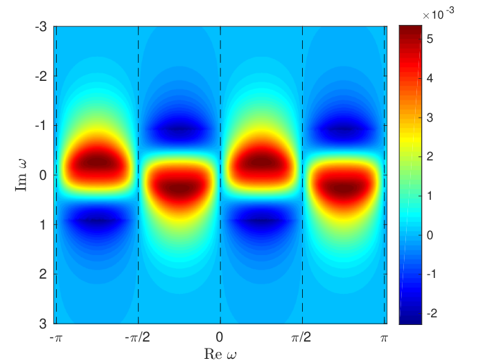
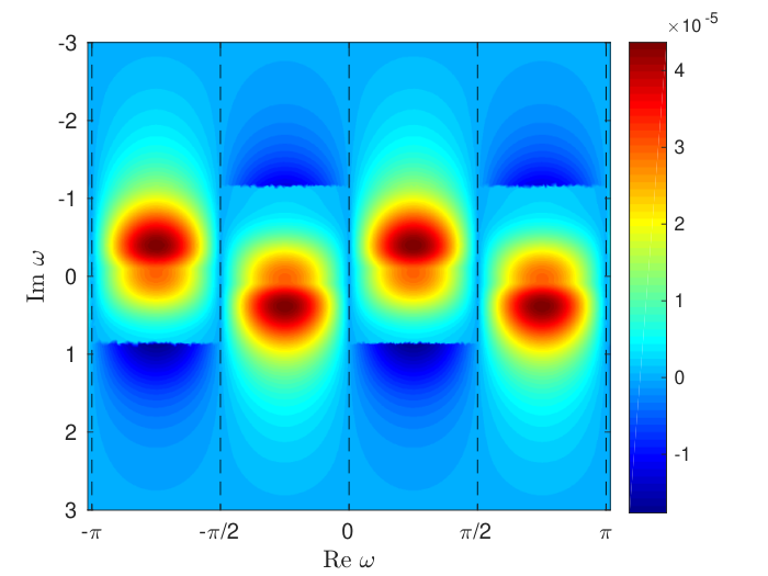
In Fig. 4, we show the maximal values
| (97) |
where we have used the best-fit values of Ref. [35] for the mixing angles. We show density plots for NH (left panel) and IH (right panel), assuming (the contour plots for are obtained from those for with the transformation ). The value of determines the value of that is needed in order to correctly reproduce the observed asymmetry. Explicitly, for NH (IH),
| (98) |
where () is the maximum value of .
Interplay between leptogenesis and dark matter results
This result clearly confirms what we anticipated, that necessarily . It should also be noticed that since the wash-out is necessarily strong, with , then and this implies the bulk of the asymmetry to be generated at temperature around [44]. From this, imposing conservatively2020 20 The factor provides a conservative lower bound, . When the lower bound is saturated, although of the lepton asymmetry generated within the interval is not converted into a baryon asymmetry, the residual small fraction of the asymmetry generated outside this interval, at higher temperatures , is still converted into a baryon asymmetry and can reproduce the observed asymmetry by further compensating with a value of lower than the one in Eq. (98). GeV, one obtains a lower bound, GeV. This lower bound on , combined with the Eq. (78) for , for initial vanishing abundance, implies an upper bound , which corresponds to . This upper bound is illustrated by the bottom panel of Fig. 2 (for , where we simply plotted vs. for different values of .
Notice also that in the case of initial vanishing abundance, Eq. (78), combined with , implies the upper bound
| (99) |
so that the scale of leptogenesis is within the range – TeV. In the case of initial thermal abundance the Eq. (74) implies the upper bound
| (100) |
so that the scale of leptogenesis is within the range – TeV.2121 21 From Eq. (17) for , that can be extended to by just replacing with an analogous quantity , one can see that this corresponds to Yukawas for initial (thermal) -abundance. This shows that imposing leptogenesis, also in this model one still needs some reduction of the neutrino Yukawa couplings compared to the other massive fermions, although slightly less than in the MSM. This reduction should be addressed within some full model, able also to specify the origin of the new interactions. In this way, we have shown that the model can explain both the DM abundance and the matter-antimatter asymmetry in a unified scenario.2222 22 In this analysis, we have neglected the contribution to the matter-antimatter asymmetry from neutrino mixing itself [5, 37, 58]. This contribution might relax the constraint on , Eq. (98), but has no impact on the obtained constraints from DM and on the properties of the high-energy neutrinos testable at IceCube.
In Table 1 we summarise the results for the allowed window on both for the quasi-degenerate and for the hierarchical case (imposing also successful leptogenesis) for the same values of as in Fig. 2.
| 2.3 | 10 | 1000 | |||
|---|---|---|---|---|---|
| 1 | NON VIABLE | — | NON VIABLE | ||
| 10 | — | 3— | — |
In Table 2 we summarise the allowed windows for the different relevant quantities of the model as indicated for the case of initial vanishing abundance and for .
| — | — | |
| — | — | |
| — | — | |
| — | — | |
| — | — |
From these two tables one can see how, in the case of a mild hierarchy , one has (for ) and . In this way, one can think of containing all new physics below , so that electroweak scale stability can be obtained with a reasonable fine-tuning without the necessity of resorting to specific solutions, such as a supersymmetric extension, to the naturalness problem. On the other hand, for one introduces a new very high energy scale, above , associated to and, if one wants to address naturalness, an extension, such as supersymmetry, would be desirable. In this case the discussed constraints would get modified along similar lines extensively studied already in the case of leptogenesis [59]. The modifications could be again parameterised in terms of a contribution to the parameter , that in the case of supersymmetry would likely be quite mild ().
4 High-energy neutrinos from DM decays and IceCube data
In this section, we finally discuss the contribution to the very high-energy neutrino flux from DM decays and its properties, comparing the predictions with the most recent IceCube high-energy starting event (HESE) data [49]. As we discussed in Section 2.3, dominantly decays through two-body and four-body processes (see Fig. 1). In this section we consider two-body decays, which occur via the mixing of with leptons, Higgs and gauge bosons, with ratio of branching ratios at the source [50], ,
| (101) |
We first discuss the flavour composition of the (almost monochromatic) neutrinos directly produced by decays, with its distinctive features, and next we derive the event energy spectrum showing two representative choices of plus an astrophysical power-law flux, that altogether predict an spectrum in good agreement with the 4-year IceCube data.
4.1 Flavour composition of hard neutrinos
Whereas gauge bosons and Higgs decays generate a softer neutrino flux with flavour composition at production, neutrinos produced directly from decays retain information of the Yukawa structure of the model (see Eq. (7)) and thus, are of particular interest. These hard neutrinos are also generated from four-body decays, , but in this case, their relevance is further diluted compared to the softer neutrinos. They have the highest kinematically allowed energies , so they are expected to produce the events from DM decays with the highest energies. Therefore, statistics permitting, by analysing the events close to the high-energy endpoint of the spectrum, information about the flavour composition and thus, about the Yukawa structure, might be inferred. However, let us note that depending on the type of interaction and on the flavour of the incoming neutrino, the deposited energy in the detector (which is the current observable used by the IceCube collaboration) might be quite different from the actual neutrino energy. Indeed, only for electron neutrino and antineutrino charged-current interactions off nucleons, the energy deposited in the detector is close to the neutrino energy. This makes the discrimination of the contribution from the neutrinos at the kinematical threshold a very challenging task, certainly not possible with current data. However, despite these intrinsic experimental difficulties in detecting these (almost monochromatic) neutrinos, we still think it is interesting to discuss their flavour composition, showing that, at production, it can be quite different from the standard mechanisms. Let us then first discuss their flavour composition at production and then at Earth.
4.1.1 Flavour composition of hard neutrinos at production
The flavour composition of monochromatic neutrinos at production is determined by the -flavour branching ratios ()
| (102) |
where or is the index corresponding to . Let us now express the ’s in terms of the low-energy neutrino parameters using the convenient orthogonal parameterisation. Taking for the third form in Eq. (7), recalling that , from the orthogonal parameterisation in Eq. (9), one straightforwardly finds
| (103) |


Notice that the denominator is . This expression clearly implies the upper bound
| (104) |
Using the C.L. lower bounds on the mixing matrix elements of the global fit of [35], one obtains
| (105) |
In the left (right) panel of Fig. 5, we show the allowed regions at C.L., C.L. and C.L. (according to the -projections provided in Refs. [35, 36]) for the flavour fractions at the source, , for NH (IH). One can see that, as expected, these plots respect the analytical bounds found in Eqs. (105).
In Section 4.2, as our benchmark scenario we consider the flavour composition of these hard neutrinos to be .
4.1.2 Flavour composition of hard neutrinos at Earth


In order to compute the final flavour composition at the detector, for all the fluxes in this work, we assume standard neutrino oscillations without exotic interactions. In this case, the neutrino flavour states produced at the source are subject to averaged oscillations in their way to the Earth. Therefore, the probability for a neutrino to arrive at the detector with flavour , if it was produced with flavour , is given by
| (106) |
and correspondingly the flavour composition at Earth, in terms of the flavour composition at the source, is given by
| (107) |
The flavour composition at Earth of the monochromatic neutrinos from DM decays is shown in Fig. 6. Looking at the plot for NH (left panel), we find the main constraint on the flavour composition to be in the electron component, which is restricted to be . This feature can be qualitatively understood in the following way. Using the fact that and the normalization of , i.e., , one can derive the following expression for the electron flavour content at the detector:
| (108) |
where , and . Thus, the total electron component at the detector is quite insensitive to the muon component at the source, and we arrive at the approximate relation
| (109) |
i.e., the electron component at the detector can be between about 0.2 and 0.6. Our model predicts for NH , i.e., also . For IH the restrictions are much less pronounced, as can be seen from Fig. 6 (right panel).


Finally, in Fig. 7, we compare the predictions of our model for the flavour composition at detection of the monochromatic neutrinos at the high-energy end of the DM decay spectrum to some of the standard reference cases. The flavour compositions at the source of the cases we consider are: (pion beam), (muon damped), and (neutron decay).
Finally, let us stress again that the ranges of the flavour composition shown in Figs. 5-7 only correspond to the almost monochromatic flux at the high-energy end of the DM decay spectrum. Given the relatively hard neutrino spectrum produced from gauge boson decays and the IceCube detector capabilities, it will be extremely challenging to single out this contribution. On the other hand, this could offer important information about the specific Yukawa structure, a definite feature of the model.
4.2 Event energy spectrum
Here we consider two representative cases for the DM mass and lifetime and compute the event spectra from two-body DM decays, as described above, expected after 4 years of data taking in IceCube. Since the DM signal alone does not represent a good fit to the entire data sample, we also consider an astrophysical contribution with a power-law flux.
The flux from DM decays has two contributions: galactic and extragalactic,
| (110) |
The decays of DM particles at cosmological distances produce a nearly isotropic neutrino and antineutrino flux, which is given by
| (111) |
where is the fraction of DM density today, is the Hubble expansion rate as a function of redshift, with and [48] (best fit values). The neutrino energy spectrum (of each flavour) from DM decays, , depends on the DM decay channel and on the DM mass, but in our notation we omit to make these dependences explicit. We use the tabulated results in Ref. [61], which include electroweak corrections [62] and were computed using PYTHIA 8.135 [63], and are provided for annihilations of DM particles with mass up to TeV (or DM decays up to TeV) and rescale them for higher masses, as done in Ref. [17]. Let us note that this procedure tends to slightly overestimate the final flux, although the precise factor depends on the decay channel and extrapolated value of the DM mass. Thus, our quoted values for the DM lifetime would need to be correspondingly scaled down by the same factor.
In addition to the extragalactic signal, DM decays in the Milky Way would also produce a flux of neutrinos and antineutrinos, which would be higher in the Southern hemisphere. Unlike the extragalactic flux, the shape of the galactic flux is not distorted by the redshifting of the signal, which implies differences also in the energy spectrum. The neutrino and antineutrino flux in a direction with galactic coordinates produced by DM decays in our own halo is given by
| (112) |
where is the DM density profile of the Milky Way as a function of the distance from the galactic centre, . For a given distance over the line-of-sight, , the galactocentric distance depends on the galactic longitude, and the galactic latitude, , as
| (113) |
where kpc is the distance from the Sun to the galactic centre [64].
For the DM distribution in our galaxy we adopt a generalised Navarro-Frenk-White [65] density profile,
| (114) |
with a scale radius kpc, and a local DM density GeV/cm3 [66]. Let us note, however, that the linear dependence on the density of the flux from DM decays, unlike the quadratic dependence of the flux from DM annihilations, implies smaller uncertainties from the poorly known shape of the DM profile and thus, the precise choice of the DM distribution in the halo is less relevant. In any case, these uncertainties would affect the normalization and the angular dependence of the flux, but not the overall shape of the energy spectrum of the galactic signal.
In Fig. 8, assuming NH and the best fit values in Eqs. (5), we show the flavour-averaged neutrino flux, , at Earth after propagation for two different DM masses and lifetimes: TeV and s (black curves) and PeV and s (red curves). 2323 23 From Table 1 one can see that, for initial vanishing abundance, the first case can explain both dark matter and leptogenesis if , one has then to resort to some of the cases discussed in Section 2.4. The second case would on the other hand require values , too large to be realistic. Both cases can explain just dark matter either, in the first case, with or, in the second case, with a plausible value . From this point of view the model certainly prefers the first case, i.e., solutions with (100 TeV). Of course for initial thermal abundance both cases would be able to explain both dark matter and matter-antimatter asymmetry of the universe with . In the left panel we depict the galactic (dashed curves) and extragalactic (dot-dashed curves) contributions, as well as the total flux (solid curves), whereas in the right panel we show the soft component (dashed curves), i.e., neutrinos from gauge bosons, Higgs and leptons decays and from the related electroweak corrections, and the hard component (dot-dashed curves), i.e., neutrinos produced at the decay vertex (including the related electroweak corrections). We note that the galactic flux dominates over the extragalactic contribution and that the soft component of the flux dominates over the hard one, except at the highest energies, close to the kinematical threshold.
Finally, we also compute the event energy spectra for these fluxes and compare them with the 4-year IceCube HESE data. As we note below, the DM decay signal cannot explain all the observed events, so another component of the flux is required. Therefore, in addition to the events from DM decays, we add the contribution from an astrophysical flux described by a power-law spectrum,
| (115) |
where is the normalization of the flux, in units of . For this astrophysical neutrino flux we assume the canonical flavour composition at Earth, .
In this work we do not attempt to perform a fit to this combined model (DM decays plus power-law flux), but simply to show some exemplary cases (see, however, Ref. [68]). Therefore, after choosing some representative values for the DM parameters, we fix the normalization of the astrophysical flux by imposing the total number of events in the electromagnetic(EM)-equivalent deposited energy range — to be equal to the sum of the DM decay and astrophysical signals plus the expected backgrounds. For the atmospheric muon and neutrino backgrounds we scale the 3-year (988 days) IceCube expected numbers [14] to obtain the 4-year (1347 days) expectations, i.e., we consider 3.3 atmospheric neutrino events and 0.6 atmospheric muon events. In order to compute the event spectra of the signal and the background contributions, we closely follow the approach of Ref. [69], which in turn represents an update of the detailed calculations described in Ref. [70] (see also Refs. [71, 72]), with some additional improvements. In this work, we use the angular and energy information of the spectra.
The event spectra for two cases: ; and ; , are shown (black histograms for the flux from DM decays and green histograms for the astrophysical flux), in Fig. 9 and Fig. 10, respectively. In both figures, we also show the background event spectra (red and blue histograms) and the total expected event spectra (purple histogram), along with the spectrum obtained using the preliminary IceCube best fit for in the EM-equivalent deposited energy interval [60 TeV 3 PeV] (gray histogram) and the 4-year data points [49]. Note that, for these values of the DM lifetime, the diffuse ray background is well above the expected DM signal [13, 23, 24].
In Fig. 9 we see that the DM signal (for TeV and ) represents the dominant contribution between 40 TeV and 150 TeV, whereas the hard astrophysical power-law flux () would explain the high-energy part of the observed event spectrum. The small low-energy excess of events with respect to the 3-year results can be nicely explained by neutrinos from DM decays within the scenario described in this paper. This also implies that the astrophysical neutrino flux does not have to be as soft as the result of the fit with only such a flux [49, 69]. On the other hand, this hard spectrum is in agreement with the results obtained for the through-going muon sample [15, 73], with a per-flavour normalization which is slightly lower, yet compatible within errors. Moreover, let us also note that the through-going muon sample is sensitive mainly to energies from a few 100 TeV to a few PeV, which are precisely the energies in which the astrophysical flux in Fig. 9 is the dominant one. In addition, this hard astrophysical spectrum would not overshoot the -ray cascade limit [74, 75, 76], or the data from air-showers arrays in galactic cases [77, 78], if sources (where neutrinos are mainly produced from pion decays) are to explain this flux.
Finally, in Fig. 10 we show the event spectra for a heavier DM candidate in combination with a softer power-law flux. In this case, the low-energy events can be explained by the astrophysical flux (), whereas the prediction of the hard DM decay signal (for PeV and ) is in agreement with the highest-energy data. However, notice that the (almost) monochromatic flux of hard neutrinos does not translate into a bump in the total event energy spectrum. This is partly due to the particular flavor composition we chose, . On the other hand, the natural kinematical cutoff in the event spectrum from DM decays (4 PeV in this case) could also explain the non-observation of events around the Glashow resonance energy ( PeV) and, in this case, the through-going muon data could be explained by the hard spectrum from DM decays2424 24 However, it is not possible to explain in this way the recently announced through-going muon event with deposited energy of 2.6 PeV [79], which is most likely produced by a 10 PeV muon neutrino (or a tau neutrino with higher energy) [80, 81], unless one considers a much heavier DM candidate. Note, as well, that the kinematical cutoff would not solve the current tension between the lack of Glashow events and the observation of this very energetic through-going muon track., instead. Let us finally note that we have not shown the results for lighter , usually quoted in the literature [17, 21, 22, 26] when considering earlier IceCube data. However, it does not represent a better agreement with data than the case shown in Fig. 10. Given the soft event spectrum resulting from the 4-year IceCube HESE data, decays from such a DM candidate, cannot explain the entire observed event spectra anymore.
5 Conclusions and final remarks
As we discussed in detail, in the scenario of cold DM from RH neutrino mixing, the same new interactions are responsible both for production and DM decays, with much stronger predictive power compared to models one can imagine where there is one kind of interaction responsible for production and another responsible for decays (e.g., some tiny small Yukawa coupling) where one has in any case freedom to reproduce both DM abundance and a contribution to IceCube neutrinos.
Therefore, finding viable solutions which are able to accommodate leptogenesis, a good DM candidate and are testable signal with neutrino telescopes is highly non-trivial. This is thanks to the possibility to generate the abundance when the is still not fully thermalised, an observation that makes viable the hierarchical case with . Physically, this relaxes the bounds since can be light with a small Yukawa coupling for higher , both things helping DM stability (see Eqs. (44) and (47)) and efficiency of production (see Eq. (30)).
In this way, even starting from initial vanishing abundance, there is an allowed range for the DM mass that, depending on the ratio , extends from GeV to about PeV (for ). On the other hand, the higher the value of , the narrower the allowed range of masses. For instance from the Fig. 2 one can see that for s, the case with and would be ruled out. More generally the upper bound for would become more and more stringent. In addition, the existence of a DM candidate nicely combines with a two-RH neutrino scenario of (resonant) leptogenesis to successfully reproduce the correct baryon asymmetry at a scale below TeV (1 PeV) for initial vanishing (thermal) abundance. In this case, the allowed range of values for narrows to TeV — 300 TeV, for , in order to have so that a lepton asymmetry can be reprocessed into a baryon asymmetry.
A contribution from decays to the high-energy neutrino flux can help reproducing the IceCube data in addition to an astrophysical component that is, in any case, necessary. Without performing a dedicated fit to the data, we have shown the contribution from DM decays to the energy spectrum for two exemplary masses, TeV and PeV, that could help explaining some of the features in the current HESE data. However, we have not investigated which case is statistically preferred (see Ref. [68]). Nevertheless, we do not find that a mass of PeV, discussed in the literature, is particularly favoured with the current data and definitely it cannot explain the entire event spectrum.
In principle, neutrinos produced directly from the decays of via retain information on the Yukawa couplings and might be singled out from the rest at energies close to . Albeit challenging, this is an interesting possibility, as the flavour composition typically differs from conventional astrophysical flavour ratios. During the next years it will be interesting to see whether more high-energy neutrino events are detected, which could support (depending on the flavor composition) the presence of a component originating from the decays of DM RH neutrinos produced by mixing with source RH neutrinos.
Acknowledgments
This paper is dedicated to the memory of Alexey Anisimov. Our work relies on many of his ideas and results. We also wish to thank Bhupal Dev, Arman Esmaili, Steve King, Stefano Morisi, Nobuchilka Okada and Apostolos Pilaftis for useful comments. PDB acknowledges financial support from the NExT/SEPnet Institute. PDB is also grateful to the Mainz Institute for Theoretical Physics (MITP) for its hospitality and its partial support during the completion of this work. PDB and PL acknowledge financial support from the STFC Consolidated Grant ST/L000296/1. SPR is supported by a Ramón y Cajal contract, by the Spanish MINECO under grants FPA2014-54459-P and SEV-2014-0398 and by the Generalitat Valenciana under grant PROMETEOII/2014/049. This project has also received funding from the European Union’s Horizon 2020 research and innovation programme under the Marie Sklodowska-Curie grant agreement No 690575 and No 674896. SPR is also partially supported by the Portuguese FCT through the CFTP-FCT Unit 777 (PEst-OE/FIS/UI0777/2013).
References
- [1] For recent reviews see, e.g., H. Davoudiasl and R. N. Mohapatra, New J. Phys. 14 (2012) 095011 [arXiv:1203.1247 [hep-ph]]; K. Petraki and R. R. Volkas, Int. J. Mod. Phys. A 28 (2013) 1330028 [arXiv:1305.4939 [hep-ph]].
- [2] P. Minkowski, Phys. Lett. B 67 (1977) 421; T. Yanagida, in Proceedings of the Workshop on Unified Theory and Baryon Number of the universe, eds. O. Sawada and A. Sugamoto (KEK, 1979) p.95; P. Ramond, Invited talk given at Conference: C79-02-25 (Feb 1979) p.265-280, CALT-68-709, hep-ph/9809459; M. Gell-Mann, P. Ramond and R. Slansky, in Supergravity, eds. P. van Niewwenhuizen and D. Freedman (North Holland, Amsterdam, 1979) Conf.Proc. C790927 p.315, PRINT-80-0576; R. Barbieri, D. V. Nanopoulos, G. Morchio and F. Strocchi, Phys. Lett. B 90 (1980) 91; R. N. Mohapatra and G. Senjanovic, Phys. Rev. Lett. 44 (1980) 912.
- [3] M. Fukugita and T. Yanagida, Phys. Lett. B 174 (1986) 45.
- [4] T. Asaka, S. Blanchet and M. Shaposhnikov, Phys. Lett. B 631 (2005) 151 [hep-ph/0503065].
- [5] E. K. Akhmedov, V. A. Rubakov and A. Y. Smirnov, Phys. Rev. Lett. 81 (1998) 1359 [hep-ph/9803255].
- [6] M. Shaposhnikov, Nucl. Phys. B 763 (2007) 49 [hep-ph/0605047].
- [7] D. Gorbunov and M. Shaposhnikov, JHEP 0710 (2007) 015 Erratum: [JHEP 1311 (2013) 101] [arXiv:0705.1729 [hep-ph]]; L. Canetti, M. Drewes and M. Shaposhnikov, New J. Phys. 14 (2012) 095012 [arXiv:1204.4186 [hep-ph]].
- [8] A. Anisimov and P. Di Bari, Phys. Rev. D 80 (2009) 073017 [arXiv:0812.5085 [hep-ph]].
- [9] B. Patt and F. Wilczek, hep-ph/0605188.
- [10] S. Palomares-Ruiz, Phys. Lett. B 665 (2008) 50 [arXiv:0712.1937 [astro-ph]].
- [11] L. Covi, M. Grefe, A. Ibarra and D. Tran, JCAP 1004 (2010) 017 [arXiv:0912.3521 [hep-ph]].
- [12] A. Esmaili, A. Ibarra and O. L. G. Peres, JCAP 1211 (2012) 034 [arXiv:1205.5281 [hep-ph]].
- [13] K. Murase and J. F. Beacom, JCAP 1210 (2012) 043 [arXiv:1206.2595 [hep-ph]].
- [14] M. G. Aartsen et al. [IceCube Collaboration], Phys. Rev. Lett. 111 (2013) 021103 [arXiv:1304.5356 [astro-ph.HE]]. M. G. Aartsen et al. [IceCube Collaboration], Science 342 (2013) 1242856 [arXiv:1311.5238 [astro-ph.HE]]; M. G. Aartsen et al. [IceCube Collaboration], Phys. Rev. Lett. 113 (2014) 101101 [arXiv:1405.5303 [astro-ph.HE]].
- [15] M. G. Aartsen et al. [IceCube Collaboration], Phys. Rev. D 89 (2014) 6, 062007 [arXiv:1311.7048 [astro-ph.HE]]. M. G. Aartsen et al. [IceCube Collaboration], Phys. Rev. Lett. 115 (2015) 8, 081102 [arXiv:1507.04005 [astro-ph.HE]].
- [16] B. Feldstein, A. Kusenko, S. Matsumoto and T. T. Yanagida, Phys. Rev. D 88 (2013) 1, 015004 [arXiv:1303.7320 [hep-ph]].
- [17] A. Esmaili and P. D. Serpico, JCAP 1311 (2013) 054 [arXiv:1308.1105 [hep-ph]].
- [18] Y. Bai, R. Lu and J. Salvado, JHEP 1601 (2016) 161 [arXiv:1311.5864 [hep-ph]].
- [19] A. Bhattacharya, M. H. Reno and I. Sarcevic, JHEP 1406 (2014) 110 [arXiv:1403.1862 [hep-ph]].
- [20] C. Rott, K. Kohri and S. C. Park, Phys. Rev. D 92 (2015) 2, 023529 [arXiv:1408.4575 [hep-ph]].
- [21] A. Esmaili, S. K. Kang and P. D. Serpico, JCAP 1412 (2014) 12, 054 [arXiv:1410.5979 [hep-ph]].
- [22] C. S. Fong, H. Minakata, B. Panes and R. Zukanovich Funchal, JHEP 1502 (2015) 189 [arXiv:1411.5318 [hep-ph]].
- [23] K. Murase, R. Laha, S. Ando and M. Ahlers, Phys. Rev. Lett. 115 (2015) 7, 071301 [arXiv:1503.04663 [hep-ph]].
- [24] A. Esmaili and P. D. Serpico, JCAP 1510 (2015) 10, 014 [arXiv:1505.06486 [hep-ph]].
- [25] S. M. Boucenna et al., JCAP 1512 (2015) 12, 055 [arXiv:1507.01000 [hep-ph]].
- [26] Y. Daikoku and H. Okada, Phys. Rev. D 91 (2015) 7, 075009 [arXiv:1502.07032 [hep-ph]].
- [27] M. Chianese, G. Miele, S. Morisi and E. Vitagliano, Phys. Lett. B 757 (2016) 251 [arXiv:1601.02934 [hep-ph]].
- [28] M. R. Fiorentin, V. Niro and N. Fornengo, arXiv:1606.04445 [hep-ph].
- [29] P. S. B. Dev, D. Kazanas, R. N. Mohapatra, V. L. Teplitz and Y. Zhang, JCAP 1608 (2016) 08, 034 arXiv:1606.04517 [hep-ph].
- [30] K. S. Babu, D. Eichler and R. N. Mohapatra, Phys. Lett. B 226 (1989) 347.
- [31] N. Cosme, L. Lopez-Honorez and M. H. G. Tytgat, Phys. Rev. D 72 (2005) 043505 [hep-ph/0506320]; N. Sahu and U. A. Yajnik, Phys. Lett. B 635 (2006) 11 [hep-ph/0509285].
- [32] P. H. Gu, M. Hirsch, U. Sarkar and J. W. F. Valle, Phys. Rev. D 79 (2009) 033010 [arXiv:0811.0953 [hep-ph]].
- [33] A. Anisimov, hep-ph/0612024.
- [34] A. Anisimov, P. Di Bari, “A Unified picture of Leptogenesis and Dark Matter”, November 2008, unpublished.
- [35] M. C. Gonzalez-Garcia, M. Maltoni and T. Schwetz, JHEP 1411 (2014) 052 [arXiv:1409.5439 [hep-ph]].
- [36] I. Esteban, M. C. Gonzalez-Garcia, M. Maltoni, I. Martinez-Soler, T. Schwetz, NuFIT 2.1: Three-neutrino fit based on data available in May 2016, http://www.nu-fit.org.
- [37] P. S. Bhupal Dev, P. Millington, A. Pilaftsis and D. Teresi, Nucl. Phys. B 886 (2014) 569 [arXiv:1404.1003 [hep-ph]]; P. S. B. Dev, P. Millington, A. Pilaftsis and D. Teresi, Nucl. Phys. B 897 (2015) 749 [arXiv:1504.07640 [hep-ph]].
- [38] J. A. Casas and A. Ibarra, Nucl. Phys. B 618 (2001) 171 [hep-ph/0103065].
- [39] S. Antusch, P. Di Bari, D. A. Jones and S. F. King, Phys. Rev. D 86 (2012) 023516 [arXiv:1107.6002 [hep-ph]].
- [40] D. J. H. Chung, E. W. Kolb and A. Riotto, Phys. Rev. D 59 (1999) 023501 [hep-ph/9802238].
- [41] F. Bezrukov, D. Gorbunov and M. Shaposhnikov, JCAP 0906 (2009) 029 [arXiv:0812.3622 [hep-ph]].
- [42] H. A. Weldon, Phys. Rev. D 26 (1982) 1394. H. A. Weldon, Phys. Rev. D 26 (1982) 2789. H. A. Weldon, Phys. Rev. D 28 (1983) 2007.
- [43] E. K. Akhmedov, hep-ph/0001264.
- [44] W. Buchmüller, P. Di Bari and M. Plümacher, Annals Phys. 315 (2005) 305 [hep-ph/0401240].
- [45] G. F. Giudice, A. Notari, M. Raidal, A. Riotto and A. Strumia, Nucl. Phys. B 685 (2004) 89 [hep-ph/0310123].
- [46] M. Shaposhnikov, JHEP 0808 (2008) 008 [arXiv:0804.4542 [hep-ph]]; A. Salvio, P. Lodone and A. Strumia, JHEP 1108 (2011) 116 [arXiv:1106.2814 [hep-ph]]; D. Besak and D. Bodeker, JCAP 1203 (2012) 029 [arXiv:1202.1288 [hep-ph]].
- [47] B. Garbrecht, F. Glowna and P. Schwaller, Nucl. Phys. B 877 (2013) 1 [arXiv:1303.5498 [hep-ph]].
- [48] P. A. R. Ade et al. [Planck Collaboration], Astron. Astrophys. 594 (2016) A13 arXiv:1502.01589 [astro-ph.CO].
- [49] M. G. Aartsen et al. [IceCube Collaboration], arXiv:1510.05223 [astro-ph.HE].
- [50] A. Atre, T. Han, S. Pascoli and B. Zhang, JHEP 0905 (2009) 030 [arXiv:0901.3589 [hep-ph]].
- [51] M. Plümacher, Nucl. Phys. B 530 (1998) 207 [hep-ph/9704231].
- [52] S. Davidson and A. Ibarra, Phys. Lett. B 535 (2002) 25 [hep-ph/0202239]; W. Buchmüller, P. Di Bari and M. Plümacher, Nucl. Phys. B 643 (2002) 367 Erratum: [Nucl. Phys. B 793 (2008) 362] [hep-ph/0205349]. S. Blanchet and P. Di Bari, JCAP 0703 (2007) 018 [hep-ph/0607330].
- [53] L. Covi, E. Roulet and F. Vissani, Phys. Lett. B 384 (1996) 169 [hep-ph/9605319].
- [54] A. Pilaftsis, Phys. Rev. D 56 (1997) 5431 [hep-ph/9707235]; A. Pilaftsis, Int. J. Mod. Phys. A 14 (1999) 1811 [hep-ph/9812256].
- [55] S. Blanchet and P. Di Bari, Nucl. Phys. B 807 (2009) 155 [arXiv:0807.0743 [hep-ph]].
- [56] S. Blanchet and P. Di Bari, JCAP 0606 (2006) 023 [hep-ph/0603107].
- [57] R. Barbieri, P. Creminelli, A. Strumia and N. Tetradis, Nucl. Phys. B 575 (2000) 61 [hep-ph/9911315]; O. Vives, Phys. Rev. D 73 (2006) 073006 [hep-ph/0512160]; E. Nardi, Y. Nir, E. Roulet and J. Racker, JHEP 0601 (2006) 164 [hep-ph/0601084]; A. Abada et l., JHEP 0609 (2006) 010 [hep-ph/0605281]; S. Blanchet and P. Di Bari, JCAP 0703 (2007) 018 [hep-ph/0607330]; S. Blanchet, P. Di Bari and G. G. Raffelt, JCAP 0703 (2007) 012 [hep-ph/0611337]. A. De Simone and A. Riotto, JCAP 0702 (2007) 005 [hep-ph/0611357]; B. Garbrecht, F. Glowna and P. Schwaller, Nucl. Phys. B 877 (2013) 1 [arXiv:1303.5498 [hep-ph]].
- [58] See M. Drewes, B. Garbrecht, D. Gueter and J. Klaric, arXiv:1606.06690 [hep-ph] and references therein.
- [59] P. Di Bari, arXiv:hep-ph/0406115; C. S. Fong, M. C. Gonzalez-Garcia, E. Nardi and J. Racker, JCAP 1012 (2010) 013 [arXiv:1009.0003 [hep-ph]]; P. Di Bari and M. Re Fiorentin, JCAP 1603 (2016) 03, 039 [arXiv:1512.06739 [hep-ph]].
- [60] L. Mohrmann [IceCube Collaboration], PoS ICRC 2015 (2016) 1066 [arXiv:1510.05223 [astro-ph.HE]].
- [61] M. Cirelli et al., JCAP 1103 (2011) 051 Erratum: [JCAP 1210 (2012) E01] [arXiv:1012.4515 [hep-ph]].
- [62] P. Ciafaloni et al., JCAP 1103 (2011) 019 [arXiv:1009.0224 [hep-ph]].
- [63] T. Sjostrand, S. Mrenna and P. Z. Skands, Comput. Phys. Commun. 178 (2008) 852 [arXiv:0710.3820 [hep-ph]].
- [64] S. Gillessen et al., Astrophys. J. 692 (2009) 1075 [arXiv:0810.4674 [astro-ph]].
- [65] L. Hernquist, Astrophys. J. 356 (1990) 359; J. F. Navarro, C. S. Frenk and S. D. M. White, Astrophys. J. 462 (1996) 563 [astro-ph/9508025]. J. F. Navarro, C. S. Frenk and S. D. M. White, Astrophys. J. 490 (1997) 493 [astro-ph/9611107].
- [66] M. Pato, F. Iocco and G. Bertone, JCAP 1512 (2015) 12, 001 [arXiv:1504.06324 [astro-ph.GA]].
- [67] G. J. Feldman and R. D. Cousins, Phys. Rev. D 57 (1998) 3873 [physics/9711021 [physics.data-an]].
- [68] A. Bhattacharya, A. Esmaili, S. Palomares-Ruiz and I. Sarcevic, in preparation.
- [69] A. C. Vincent, S. Palomares-Ruiz and O. Mena, Phys. Rev. D 94 (2016) 2, 023009 arXiv:1605.01556 [astro-ph.HE].
- [70] S. Palomares-Ruiz, A. C. Vincent and O. Mena, Phys. Rev. D 91 (2015) 10, 103008 [arXiv:1502.02649 [astro-ph.HE]].
- [71] O. Mena, S. Palomares-Ruiz and A. C. Vincent, Phys. Rev. Lett. 113 (2014) 091103 [arXiv:1404.0017 [astro-ph.HE]].
- [72] S. Palomares-Ruiz, O. Mena and A. C. Vincent, Proceedings of the International Conference on High Energy Physics 2014 (ICHEP 2014), Nucl. Part. Phys. Proc. 273-275 (2016) 433-439 [arXiv:1411.2998 [astro-ph.HE]]. A. C. Vincent, S. P. Ruiz and O. Mena, Proceedings of the 50th Rencontres de Moriond Electroweak interactions and unified theories, pp. 407-412, 2015, arXiv:1505.03355 [astro-ph.HE]. S. Palomares-Ruiz, Proceedings of the 30th International Workshop on High Energy Physics: Particle and Astroparticle Physics, Gravitation and Cosmology: Predictions, Observations and New Projects (IHEP 2014), pp. 271-275, 2015.
- [73] M. G. Aartsen et al. [IceCube Collaboration], Astrophys. J. 809 (2015) 1, 98 [arXiv:1507.03991 [astro-ph.HE]].
- [74] K. Murase, M. Ahlers and B. C. Lacki, Phys. Rev. D 88 (2013) 12, 121301 [arXiv:1306.3417 [astro-ph.HE]].
- [75] X. C. Chang and X. Y. Wang, Astrophys. J. 793 (2014) 2, 131 [arXiv:1406.1099 [astro-ph.HE]].
- [76] S. Ando, I. Tamborra and F. Zandanel, Phys. Rev. Lett. 115 (2015) 22, 221101 [arXiv:1509.02444 [astro-ph.HE]].
- [77] M. Ahlers and K. Murase, Phys. Rev. D 90 (2014) 2, 023010 [arXiv:1309.4077 [astro-ph.HE]].
- [78] O. E. Kalashev and S. V. Troitsky, JETP Lett. 100 (2015) 12, 761 [arXiv:1410.2600 [astro-ph.HE]].
- [79] S. Schoenen and L. Raedel. 2015. L. [IceCube Collaboration], Astronomer’s Telegram, 7856, 1.
- [80] M. D. Kistler and R. Laha, arXiv:1605.08781 [astro-ph.HE].
- [81] M. G. Aartsen et al. [IceCube Collaboration], arXiv:1607.08006 [astro-ph.HE].