In this paper we present an algorithm for computing a middle levels Gray code in optimal time and space.

Clearly, the running time of this algorithm is ${\mathcal{O}}(1)$ on average per generated bitstring for $\ell=\Omega(n)$, and the required initialization time ${\mathcal{O}}(n)$ and the required space ${\mathcal{O}}(n)$ are also optimal.

We implemented our new middle levels Gray code in C++, and we invite the reader to experiment with this code, which can be found and run on the Combinatorial Object Server website [cos]. As a benchmark, we used this code to compute a middle levels Gray code for $n=19$ in 20 minutes on a standard desktop computer. This is by a factor of $72$ faster than the 24 hours reported in [MN18] for the algorithm from Theorem 2, and by four orders of magnitude faster than the 164 days previously needed for a brute-force search [SA11]. Note that a middle levels Gray code for $n=19$ consists of $N=137.846.528.820\approx 10^{11}$ bitstrings. For comparison, a program that only consists of a loop with a counting variable running from $1,\ldots,N$ and nothing else was only by a factor of $5$ faster (4 minutes) than our middle levels Gray code computation on the same hardware. Roughly speaking, we need about 5 arithmetic operations for producing the next bitstring in the Gray code.

We now also obtain efficient algorithms for a number of related Gray codes that have been constructed using Theorem 1 as an induction basis. These Gray codes consist of several combined middle levels Gray codes of smaller dimensions. Specifically, it was a long-standing problem (see [Sim91, Hur94, Che00, Che03]) to construct a Gray code that lists all $k$-element and $(n-k)$-element subsets of $[n]$, where $n\geq 2k+1$, by either adding or removing $n-2k$ elements in each step. This was solved in [MS17], and using Theorem 3 this construction can now be turned into an efficient algorithm. Moreover, in [GM18] Theorem 3 is used to derive constant-time algorithms for generating minimum-change listings of all $n$-bit strings whose weight is in some interval $[k,l]$, $0\leq k\leq l\leq n$, a far-ranging generalization of the middle levels conjecture and the classical problems (2) and (3) mentioned before.

In this work we restrict our attention to computing one particular ‘canonical’ middle levels Gray code for any $n\geq 1$, even though we know from [Müt16] that there are double-exponentially many different ones (recall [MN18, Remark 3]).

We shall see that most steps of our algorithm require only constant time ${\mathcal{O}}(1)$ in the worst case to generate the next bitstring, but after every sequence of $\Theta(n)$ such ‘fast’ steps, a ‘slow’ step which requires time $\Theta(n)$ is encountered, yielding constant average time performance. Therefore, our algorithm could easily be transformed into a loopless algorithm, i.e., one with a ${\mathcal{O}}(1)$ worst case bound for each generated bitstring, by introducing an additional FIFO queue of size $\Theta(n)$ and by simulating the original algorithm such that during every sequence of $d$ ‘fast’ steps, $d-1$ results are stored in the queue and only one of them is returned, and during the ‘slow’ steps the queue is emptied at the same speed. For this the constant $d$ must be chosen so that the queue is empty when the ‘slow’ steps are finished. This idea of delaying the output to achieve a loopless algorithm is also used in [HR16] (see also [Sed77, Section 1]). Even though the resulting algorithm would indeed be loopless, it would still be slower than the original algorithm, as it produces every bitstring only after it was produced in the original algorithm, due to the delay caused by the queue and the additional instructions for queue management. In other words, the hidden constant in the ${\mathcal{O}}(1)$ bound for the modified algorithm is higher than for the original algorithm, so this loopless algorithm is only of theoretical interest, and we will not discuss it any further.

Our algorithm for computing a middle levels Gray code implements the strategy of the short proof of Theorem 1 presented in [GMN18]. In the most basic version, the algorithm computes several short cycles that together visit all bitstrings of length $2n+1$ with weight $n$ or $n+1$. We then modify a few steps of the algorithm so that these short cycles are joined to a Gray code that visits all bitstrings consecutively.

Let us briefly discuss the main differences between the algorithms from Theorem 2 and Theorem 3 and the improvements that save us a factor of $n$ in the running time. At the lowest level, the algorithm from Theorem 2 consists of a rather unwieldy recursion, which for any given bitstring computes the next one in a middle levels Gray code. This recursion runs in time $\Theta(n)$, and therefore represents one of the bottlenecks in the running time. In addition, there are various high-level functions that are called every $\Theta(n)$ many steps and run in time $\Theta(n^{2})$, and which therefore also represent $\Theta(n)$ bottlenecks. These high-level functions control which subsets of bitstrings are visited in which order, to make sure that each bitstring is visited exactly once.

To overcome these bottlenecks, we replace the recursion at the lowest level by a simple combinatorial technique, first proposed in [MSW18] and heavily used in the short proof of Theorem 1 presented in [GMN18]. This technique allows us to compute for certain ‘special’ bitstrings that are encountered every $\Theta(n)$ many steps, a sequence of bit positions to be flipped during the next $\Theta(n)$ many steps. Computing such a flip sequence can be done in time $\Theta(n)$, and when this is accomplished each subsequent step takes only constant time: We simply flip the precomputed positions one after the other, until the next ‘special’ bitstring is encountered and the flip sequence has to be recomputed. The high-level functions in the new algorithm are very similar as in the old one. We cut down their running time by a factor of $n$ (from quadratic to linear) by using more sophisticated data structures and by resorting to well-known algorithms such as Booth’s linear-time algorithm [Boo80] for computing the lexicographically smallest rotation of a given string.

In Section 2 we introduce important definitions that will be used throughout the paper. In Section 3 we present our new middle levels Gray code algorithm. In Section 4 we prove the correctness of the algorithm, and in Section 5 we discuss how to implement it to achieve the claimed runtime and space bounds.

In this section we describe a set of disjoint paths ${\mathcal{P}}_{n}$ that together visit all vertices of the graph $H_{n}$. The starting vertices of these paths are the vertices $x\in D_{n}$, and in the following we describe a rule $\sigma(x)$ that specifies the sequence of bit positions to be flipped along the path starting at $x$. To compute the flip sequence $\sigma(x)$ for a given vertex $x\in D_{n}$, we interpret $x$ as a Dyck path, and we alternatingly flip ${\searrow}$-steps and ${\nearrow}$-steps of this Dyck path (corresponding to 0s and 1s in $x$, respectively). Specifically, for $x\in D_{n}$ we consider the canonical decomposition $x=1u0v$ and define $a:=1$, $b:=|u|+2$ and

Note that in (1a), the integers $a$ and $b$ are the positions of 1 and 0 in the canonical decomposition $x=1u0v$. Similarly, in (1b), the integers $a$ and $b$ are the positions of 1 and 0 in the canonical decomposition of the substring $x^{\prime}=1u^{\prime}0v^{\prime}$ of $x$, and those positions are with respect to the entire string $x$ (the index of $\sigma_{a}$ tracks the starting position of $x^{\prime}$ in $x$).

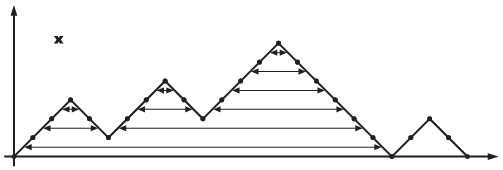
In words, the sequence $\sigma(x)$ defined in (1a) first flips the ${\searrow}$-step immediately after the subpath $u$ (at position $b$ of $x$), then the ${\nearrow}$-step immediately before the subpath $u$ (at position $1$), and then recursively steps of $u$. No steps of $v$ are flipped at all. The sequence $\sigma_{a}(x^{\prime})$ defined in (1b) first flips the ${\searrow}$-step immediately after the subpath $u^{\prime}$ (at position $b$ of $x$), then the ${\nearrow}$-step immediately before the subpath $u^{\prime}$ (at position $a$), then recursively steps of $u^{\prime}$, then again the step immediately to the left of $x^{\prime}$ (which is not part of $x^{\prime}$, hence the index $a-1$), then again the step immediately to the right of $u^{\prime}$ (at position $b$), and finally recursively steps of $v^{\prime}$; see Figure 2. The recursion $\sigma(x)$ has a straightforward combinatorial interpretation: We consider the Dyck subpaths of the Dyck path $x$ with increasing height levels and from left to right on each level, and we process them in two phases. In phase 1, we flip the steps of each such subpath alternatingly between the rightmost and leftmost step, moving upwards. In phase 2, we flip the steps alternatingly between the leftmost and rightmost step, moving downwards again. We emphasize here that during the recursive computation of $\sigma(x)$, no steps of $x$ are ever flipped, but we always consider the same Dyck path and its Dyck subpaths as function arguments.

Note that by the definition (1), we have $|\sigma(x)|=2|u|+2$, where $x=1u0v$ is the canonical decomposition. We let $P_{\sigma}(x)$ denote the sequence of vertices obtained by starting at the vertex $x$ and flipping bits one after the other according to the sequence $\sigma(x)$. The following properties were proved in [GMN18, Proposition 2].

1. (i)

   For any $x\in D_{n}$, $P_{\sigma}(x)$ is a path in the graph $H_{n}$. Moreover, all paths in ${\mathcal{P}}_{n}:=\{P_{\sigma}(x)\mid x\in D_{n}\}$ are disjoint, and together they visit all vertices of $H_{n}$.

2. (ii)

   For any first vertex $x\in D_{n}$, considering the canonical decomposition $x=1u0v$, the last vertex of $P_{\sigma}(x)$ is given by $u01v\in D_{n}^{-}$. Consequently, the sets of first and last vertices of the paths ${\mathcal{P}}_{n}$ are given by $D_{n}$ and $D_{n}^{-}$, respectively.

Table 1 shows the five paths in ${\mathcal{P}}_{n}$ for $n=3$.

To compute a Hamilton cycle in the middle levels graphs $G_{n}$, we apply small local modifications to certain pairs of paths from ${\mathcal{P}}_{n}$, giving us additional freedom in combining an appropriate set of paths to a Hamilton cycle. Specifically, we say that $x,y\in D_{n}$ form a flippable pair $(x,y)$, if

for some $w,v\in D$. In terms of rooted trees, the tree $y$ is obtained from $x$ by removing the pending edge that leads to the leftmost child of the leftmost child of the root, and by attaching this edge leftmost to the root; see Figure 3 (recall the correspondence between Dyck paths and rooted trees explained in Section 2). We denote this operation by $\tau$ and write $y=\tau(x)$. The preimage $T_{n}\subseteq D_{n}$ of the mapping $\tau$ are all rooted trees with $n$ edges of the form $x=110w0v$, and the image of $\tau$ are all rooted trees of the form $y=101w0v$, where $w,v\in D$; see Figure 6. Note that these two sets are disjoint.

Evaluating the recursion (1) for the bitstrings in a flippable pair $(x,y)$ as in (2) yields

where $b:=|w|+2$. It follows that the paths $P_{\sigma}(x)$ and $P_{\sigma}(y)$ intersect a common 6-cycle $C_{6}(x,y)$ in the graph $H_{n}$ as shown in Figure 4. Specifically, this 6-cycle can be encoded by

where the six cycle vertices are obtained by substituting the three $*$s by all six combinations of symbols from $\{0,1\}$ that use each symbol at least once. Consequently, taking the symmetric difference of the edge sets of $P_{\sigma}(x)$ and $P_{\sigma}(y)$ with the 6-cycle $C_{6}(x,y)$ yields two paths on the same vertex set as $P_{\sigma}(x)$ and $P_{\sigma}(y)$, but with interchanged end vertices. The resulting paths $P_{\widetilde{\sigma}}(x)$ and $P_{\widetilde{\sigma}}(y)$ have flip sequences

and we refer to these two paths as flipped paths corresponding to the flippable pair $(x,y)$.

In this section we present our algorithm to compute a Hamilton cycle in the middle levels graph $G_{n}$ (Algorithm 1). The Hamilton cycle is obtained by combining paths that are computed via the flip sequences $\sigma$ and ${\widetilde{\sigma}}$. We use the decomposition of $G_{n}$ into $H_{n}\,0$, $\overline{\rev}(H_{n})\,1$, plus the matching $M_{n}$ discussed in Section 2; see Figure 5. By property (ii) from Section 3.1, the sets of first and last vertices of the paths ${\mathcal{P}}_{n}$ are $D_{n}$ and $D_{n}^{-}$, respectively. It is easy to see that these two sets are preserved under the mapping $\overline{\rev}$. Together with property (i) from Section 3.1 it follows that

with $M_{n}^{\prime}:=\{(x0,x1)\mid x\in D_{n}\cup D_{n}^{-}\}\subseteq M_{n}$ is a 2-factor in the middle levels graph. A 2-factor in a graph is a collection of disjoint cycles that together visit all vertices of the graph. Note that along each of the cycles in the 2-factor, the paths from ${\mathcal{P}}_{n}\,0$ are traversed in forward direction, and the paths from $\overline{\rev}({\mathcal{P}}_{n})\,1$ in backward direction. Observe also that the definition of flippable pairs given in Section 3.2 allows us to replace in the definition (5) any two paths $P_{\sigma}(x)$ and $P_{\sigma}(y)$ from ${\mathcal{P}}_{n}$ for which $(x,y)$ forms a flippable pair by the corresponding flipped paths $P_{\widetilde{\sigma}}(x)$ and $P_{\widetilde{\sigma}}(y)$, yielding another 2-factor. Specifically, if the paths we replace lie on two different cycles, then the replacement will join the two cycles to one cycle. The final algorithm makes all those choices such that the resulting 2-factor consists only of a single cycle, i.e., a Hamilton cycle.

For the rest of the paper we will focus on proving that the algorithm $\HamCycle$, described in Algorithm 1, implies Theorem 3. $\HamCycle$ is called with three input parameters: $n$ determines the length $2n+1$ of the bitstrings, $x$ is the starting vertex of the Hamilton cycle and must have weight $n$ or $n+1$, and $\ell$ is the number of vertices to visit along the cycle.

The variable $y$ is the current vertex along the cycle, and the variable $i$ counts the number of vertices that have already been visited. The calls $\Visit(y)$ in lines 1, 1, 1 and 1 indicate where a function using our Hamilton cycle algorithm could perform further operations on the current vertex $y$. Each time a vertex along the cycle is visited, we increment $i$ and check whether the desired number $\ell$ of vertices has been visited (lines 1, 1, 1 and 1).

We postpone the definition of the functions $\Init$ and $\IsFlipTree$ called in lines 1 and 1 a little bit, and assume for a moment that the input vertex $x$ of the middle levels graph $G_{n}$ has the form $x=z0$ with $z\in D_{n}$. In this case the variables $y$ and $i$ will be initialized to $y:=x$ and $i:=1$ in line 1. Let us also assume that the return value of $\IsFlipTree$ called in line 1 is always $\false$. With these simplifications, the algorithm $\HamCycle$ computes exactly the 2-factor ${\mathcal{C}}_{n}$ defined in (5) in the middle levels graph $G_{n}$.

Indeed, one complete execution of the first for-loop corresponds to following one path from the set ${\mathcal{P}}_{n}\,0$ in the graph $H_{n}\,0$ starting at its first vertex and ending at its last vertex, and one complete execution of the second for-loop corresponds to following one path from the set $\overline{\rev}({\mathcal{P}}_{n})\,1$ in the graph $\overline{\rev}(H_{n})\,1$ starting at its last vertex and ending at its first vertex. At the intermediate steps in lines 1 and 1, the last bit is flipped. These flips correspond to traversing an edge from the matching $M_{n}^{\prime}$. The paths ${\mathcal{P}}_{n}$ are computed in lines 1 and 1 using the recursion $\sigma$, and the resulting flip sequences are applied in the two inner for-loops (line 1 and 1). Note that if a path from the set ${\mathcal{P}}_{n}$ has $y\in D_{n}^{-}$ as a last vertex and if $y=u01v$ is the canonical decomposition, then $\overline{\rev}$ maps the last vertex of the path $P\in{\mathcal{P}}_{n}$ that has $1\,\overline{\rev}(v)\,0\,\overline{\rev}(u)$ as first vertex onto $y$. This is a consequence of property (ii) from Section 3.1, from which we obtain that the last vertex of $P$ is $\overline{\rev}(v)\,01\,\overline{\rev}(u)$, and applying $\overline{\rev}$ to this vertex indeed yields $y$. From these observations and the definitions in lines 1, 1 and 1 it follows that the paths in the second set on the right hand side of (5) are indeed traversed in backward direction (starting at the last vertex and ending at the first vertex).

We now explain the significance of the function $\IsFlipTree$ called in line 1 of our algorithm. This function interprets the current first vertex $y^{-}\in T_{n}\subseteq D_{n}$ or $\tau^{-1}(y^{-})\in T_{n}$ as a rooted tree, and whenever it returns $\true$, then instead of computing the flip sequence $\sigma(y^{-})$ in line 1, the algorithm computes the modified flip sequence ${\widetilde{\sigma}}(y^{-})$ in line 1. Consequently, the function $\IsFlipTree$ controls which pairs of paths from ${\mathcal{P}}_{n}$, whose first vertices form a flippable pair, are replaced by the corresponding flipped paths, so that the resulting 2-factor in the middle levels graph $G_{n}$ is a Hamilton cycle. Observe that these modifications only apply to the set ${\mathcal{P}}_{n}\,0$, but not to the set $\overline{\rev}({\mathcal{P}}_{n})\,1$ on the right hand side of (5).

The function $\IsFlipTree$ therefore encapsulates the core ‘intelligence’ of our Hamilton cycle algorithm. We define this function and the function $\Init$ in the next two sections. The correctness proof for the algorithm $\HamCycle$ is provided in Section 4 below.

To define the Boolean function $\IsFlipTree$, we need a few more definitions related to trees.

Leaves, stars, and tree center. Any vertex of degree 1 of a tree is called a leaf. We call a leaf thin, if its unique neighbor in the tree has degree 2. A star is a tree in which all but at most one vertex are leaves. The center of a tree is the set of vertices that minimize the maximum distance to any other vertex. Any tree either has a unique center vertex, or two center vertices that are adjacent. For a rooted tree, these notions are independent of the vertex orderings. Also note that the root of a rooted tree can be a leaf.

The following auxiliary function $\troot$ computes a canonically rooted version of a given rooted tree. Formally, for any tree $x\in D_{n}$ and any integer $r\geq 0$ the return value of $\troot(\trot^{r}(x))$ is the same rotated version of $x$. In the following functions, all comparisons between trees are performed using the bitstring representation.

The function $\troot$: Given a tree $x\in D_{n}$, first compute its center vertex/vertices. If there are two centers $c_{1}$ and $c_{2}$, then let $x^{\prime}$ be the tree obtained by rooting $x$ so that $c_{1}$ is the root and $c_{2}$ its leftmost child, let $x^{\prime\prime}$ be the tree obtained by rooting $x$ so that $c_{2}$ is the root and $c_{1}$ its leftmost child, and return the tree from $\{x^{\prime},x^{\prime\prime}\}$ with the lexicographically smaller bitstring representation. If the center $c$ is unique, then let $y_{1},y_{2},\ldots,y_{k}$ be the subtrees of $x$ rooted at $c$. Consider the bitstring representations ot these subtrees, and compute the lexicographically smallest rotation of the string $(-1,y_{1},-1,y_{2},-1,\ldots,-1,y_{k})$ using Booth’s algorithm [Boo80]. Here $-1$ is an additional symbol that is lexicographically smaller than 0 and 1, ensuring that the lexicographically smallest string rotation starts at a tree boundary. Let ${\widehat{x}}$ be the tree obtained by rooting $x$ at $c$ such that the subtrees $y_{1},\ldots,y_{k}$ appear exactly in this lexicographically smallest ordering, and return ${\widehat{x}}$.

We are now ready to define the function $\IsFlipTree$.

The function $\IsFlipTree$: Given a tree $x\in T_{n}$, return $\false$ if $x$ is a star. Otherwise compute ${\widehat{x}}:=\troot(x)$. If $x$ has a thin leaf, then let $x^{\prime}$ be the tree obtained by rotating ${\widehat{x}}$ until it has the form $x^{\prime}=1100v$ for some $v\in D$. Return $\true$ if $x=x^{\prime}$, and return $\false$ otherwise. If $x$ has no thin leaf, then let $x^{\prime}$ be the tree obtained by rotating ${\widehat{x}}$ until it has the form $x^{\prime}=1(10)^{k}0v$ for some $k\geq 2$ and $v\in D$. Return $\true$ if $x=x^{\prime}$ and if the condition $v=(10)^{l}$ implies that $l\geq k$, and return $\false$ otherwise.

It remains to define the function $\Init(n,x,\ell)$ called in line 1 of the algorithm $\HamCycle$. This function moves forward along the Hamilton cycle from the given vertex $x$ in $G_{n}$ and visits all vertices until the first vertex of the form $z0$ with $z\in D_{n}$ is encountered. We then initialize the current vertex as $y:=z0$, and set the vertex counter $i$ to the number of vertices visited along the cycle from $x$ to $y$. The parameter $\ell$ is passed, as it might be so small that the termination condition is already reached on this initial path.

The first task is to compute, for the given vertex $x$, which path $P_{\sigma}(y)\,0$ or $\overline{\rev}(P_{\sigma}(y))\,1$ the vertex $x$ is contained in. With this information we can run essentially one iteration of the while-loop of the algorithm $\HamCycle$, after which we reach the first vertex of the form $z0$ with $z\in D_{n}$.

To achieve this, if the last bit of $x$ is 0, i.e., $x=z0$, then we compute $y\in D_{n}$ such that $z\in P_{\sigma}(y)$ as follows: We consider the point(s) with lowest height on the lattice path $z$. If the lowest point of $z$ is unique, then we partition $z$ uniquely as

for some $d\geq 0$ and $u_{1},\ldots,u_{d},v_{1},\ldots,v_{d},w\in D$. In all four cases, a straightforward calculation using the definition (1) shows that

is indeed the first vertex of the path $P_{\sigma}(y)$ that contains the vertex $z$. In particular, if $z\in D_{n}$, then $d=0$ and $y=z=1w0v$.

If the last bit of $x$ is 1, i.e., $x=z1$, then we compute $y\in D_{n}$ such that $z\in\overline{\rev}(P_{\sigma}(y))$ by applying the previous steps to the vertex $\overline{\rev}(z)$.

For more details how the function $\Init$ is implemented, see our C++ implementation [cos].

For any $x\in D_{n}$, the flip sequence $\sigma(x)$ can be computed in linear time. To achieve this, we precompute an array of bidirectional pointers below the Dyck subpaths of $x$ between corresponding pairs of an ${\nearrow}$-step and ${\searrow}$-step on the same height; see Figure 8. Using these pointers, each canonical decomposition operation encountered in the recursion (1) can be performed in constant time, so that the overall running time of the recursion is ${\mathcal{O}}(n)$. Clearly, the sequence ${\widetilde{\sigma}}(x)$ can also be computed in time ${\mathcal{O}}(n)$ by modifying the sequence $\sigma(x)$ as described in (4) in constantly many positions. Obviously, the functions $\overline{\rev}(u)$ and $\overline{\rev}(v)$ called in line 1 can also be computed in time ${\mathcal{O}}(n)$.

To compute the functions $\troot$ and $\IsFlipTree$, we first convert the given bitstring $x\in D_{n}$ to a tree in adjacency list representation, which can clearly be done in time ${\mathcal{O}}(n)$; recall the correspondence between Dyck paths and rooted trees from Figure 1. The adjacency list representation allows us to compute the center vertex/vertices in linear time by removing leaves in rounds until only a single vertex or a single edge is left (see [Ski08]). Moreover, it allows us to perform each rotation operation $\trot$ in constant time, and a full tree rotation in time ${\mathcal{O}}(n)$. Booth’s algorithm to compute the lexicographically smallest string rotation also runs in linear time [Boo80]. This gives the bound ${\mathcal{O}}(n)$ for the time spent in the functions $\troot$ and $\IsFlipTree$.

It was shown in [GMN18, Proposition 2] that the distance between any two consecutive vertices of the form $x0$ and $y0$ with $x,y\in D_{n}$ on a cycle of the 2-factor ${\mathcal{C}}_{n}$ is exactly $4n+2$. Moreover, replacing a path $P_{\sigma}(x)$ in the first set on the right hand side of (5) by the path $P_{\widetilde{\sigma}}(x)$ does not change this distance; recall Figure 4. It follows that in each iteration of the while-loop of our algorithm $\HamCycle$, exactly $4n+2$ vertices are visited. Combining this with the time bounds ${\mathcal{O}}(n)$ derived for the functions $\sigma$, ${\widetilde{\sigma}}$, $\overline{\rev}$ and $\IsFlipTree$ that are called once or twice during each iteration of the while-loop, we conclude that the while-loop takes time ${\mathcal{O}}(\ell+n)$ to visit $\ell$ vertices of the Hamilton cycle.

The function $\Init$ takes time ${\mathcal{O}}(n)$, as the partitions (6) can be computed in linear time, and as we visit at most linearly many vertices in this function (every path in ${\mathcal{P}}_{n}$ has only length ${\mathcal{O}}(n)$).

Combining the time bounds ${\mathcal{O}}(n)$ for the initialization phase and the time ${\mathcal{O}}(\ell+n)$ spent in the while-loop, we obtain the claimed overall bound ${\mathcal{O}}(\ell+n)$ for the algorithm $\HamCycle$.

Throughout our algorithm, we only store constantly many bitstrings of length $2n$, rooted trees with $n$ edges, and flip sequences of length at most $4n+2={\mathcal{O}}(n)$, proving that the entire space needed is ${\mathcal{O}}(n)$.

References

- [BER76] J. Bitner, G. Ehrlich, and E. Reingold. Efficient generation of the binary reflected Gray code and its applications. Comm. ACM, 19(9):517–521, 1976.
- [Boo80] K. S. Booth. Lexicographically least circular substrings. Inform. Process. Lett., 10(4-5):240–242, 1980.
- [BW84] M. Buck and D. Wiedemann. Gray codes with restricted density. Discrete Math., 48(2-3):163–171, 1984.
- [Che00] Y. Chen. Kneser graphs are Hamiltonian for . J. Combin. Theory Ser. B, 80(1):69–79, 2000.
- [Che03] Y. Chen. Triangle-free Hamiltonian Kneser graphs. J. Combin. Theory Ser. B, 89(1):1–16, 2003.
- [cos] The Combinatorial Object Server: http://combos.org.
- [Cum66] R. L. Cummins. Hamilton circuits in tree graphs. IEEE Trans. Circuit Theory, CT-13:82–90, 1966.
- [Der75] N. Dershowitz. A simplified loop-free algorithm for generating permutations. Nordisk Tidskr. Informationsbehandling (BIT), 15(2):158–164, 1975.
- [DG12] P. Diaconis and R. Graham. Magical mathematics. Princeton University Press, Princeton, NJ, 2012. The mathematical ideas that animate great magic tricks, With a foreword by Martin Gardner.
- [DKS94] D. A. Duffus, H. A. Kierstead, and H. S. Snevily. An explicit -factorization in the middle of the Boolean lattice. J. Combin. Theory Ser. A, 65(2):334–342, 1994.
- [DSW88] D. Duffus, B. Sands, and R. Woodrow. Lexicographic matchings cannot form Hamiltonian cycles. Order, 5(2):149–161, 1988.
- [Ehr73] G. Ehrlich. Loopless algorithms for generating permutations, combinations, and other combinatorial configurations. J. Assoc. Comput. Mach., 20:500–513, 1973.
- [EHR84] P. Eades, M. Hickey, and R. C. Read. Some Hamilton paths and a minimal change algorithm. J. Assoc. Comput. Mach., 31(1):19–29, 1984.
- [EM84] P. Eades and B. McKay. An algorithm for generating subsets of fixed size with a strong minimal change property. Inform. Process. Lett., 19(3):131–133, 1984.
- [FT95] S. Felsner and W. T. Trotter. Colorings of diagrams of interval orders and -sequences of sets. Discrete Math., 144(1-3):23–31, 1995. Combinatorics of ordered sets (Oberwolfach, 1991).
- [GM18] P. Gregor and T. Mütze. Trimming and gluing Gray codes. Theoret. Comput. Sci., 714:74–95, 2018.
- [GMN18] P. Gregor, T. Mütze, and J. Nummenpalo. A short proof of the middle levels theorem. Discrete Analysis, 8:12 pp., 2018.
- [Gow17] W. T. Gowers. Probabilistic combinatorics and the recent work of Peter Keevash. Bull. Amer. Math. Soc. (N.S.), 54(1):107–116, 2017.
- [Gra53] F. Gray. Pulse code communication, 1953. March 17, (filed Nov. 1947). U.S. Patent 2,632,058.
- [GŠ10] P. Gregor and R. Škrekovski. On generalized middle-level problem. Inform. Sci., 180(12):2448–2457, 2010.
- [Hav83] I. Havel. Semipaths in directed cubes. In Graphs and other combinatorial topics (Prague, 1982), volume 59 of Teubner-Texte Math., pages 101–108. Teubner, Leipzig, 1983.
- [HH72] C. A. Holzmann and F. Harary. On the tree graph of a matroid. SIAM J. Appl. Math., 22:187–193, 1972.
- [HKRR05] P. Horák, T. Kaiser, M. Rosenfeld, and Z. Ryjáček. The prism over the middle-levels graph is Hamiltonian. Order, 22(1):73–81, 2005.
- [HR16] F. Herter and G. Rote. Loopless Gray code enumeration and the tower of Bucharest. In 8th International Conference on Fun with Algorithms, FUN 2016, June 8-10, 2016, La Maddalena, Italy, pages 19:1–19:19, 2016.
- [Hur94] G. Hurlbert. The antipodal layers problem. Discrete Math., 128(1-3):237–245, 1994.
- [Joh63] S. M. Johnson. Generation of permutations by adjacent transposition. Math. Comp., 17:282–285, 1963.
- [Joh04] J. R. Johnson. Long cycles in the middle two layers of the discrete cube. J. Combin. Theory Ser. A, 105(2):255–271, 2004.
- [Kam67] T. Kamae. The existence of a Hamilton circuit in a tree graph. IEEE Trans. Circuit Theory, CT-14:279–283, 1967.
- [Knu11] D. E. Knuth. The Art of Computer Programming. Vol. 4A. Combinatorial Algorithms. Part 1. Addison-Wesley, Upper Saddle River, NJ, 2011.
- [KT88] H. A. Kierstead and W. T. Trotter. Explicit matchings in the middle levels of the Boolean lattice. Order, 5(2):163–171, 1988.
- [LRvBR93] J. M. Lucas, D. Roelants van Baronaigien, and F. Ruskey. On rotations and the generation of binary trees. J. Algorithms, 15(3):343–366, 1993.
- [Luc87] J. M. Lucas. The rotation graph of binary trees is Hamiltonian. J. Algorithms, 8(4):503–535, 1987.
- [MN17] T. Mütze and J. Nummenpalo. A constant-time algorithm for middle levels Gray codes. In Proceedings of the Twenty-Eighth Annual ACM-SIAM Symposium on Discrete Algorithms, SODA 2017, Barcelona, Spain, Hotel Porta Fira, January 16-19, pages 2238–2253, 2017.
- [MN18] T. Mütze and J. Nummenpalo. Efficient computation of middle levels Gray codes. ACM Trans. Algorithms (TALG), 14(2):29 pp., 2018. An extended abstract appeared in the Proceedings of the European Symposium on Algorithms (ESA 2015).
- [MS17] T. Mütze and P. Su. Bipartite Kneser graphs are Hamiltonian. Combinatorica, 37(6):1207–1219, 2017.
- [MSW18] T. Mütze, C. Standke, and V. Wiechert. A minimum-change version of the Chung-Feller theorem for Dyck paths. European J. Combin., 69:260–275, 2018.
- [Müt16] T. Mütze. Proof of the middle levels conjecture. Proc. London Math. Soc., 112(4):677–713, 2016.
- [MW12] T. Mütze and F. Weber. Construction of 2-factors in the middle layer of the discrete cube. J. Combin. Theory Ser. A, 119(8):1832–1855, 2012.
- [NW75] A. Nijenhuis and H. S. Wilf. Combinatorial algorithms. Academic Press, New York-London, 1975. Computer Science and Applied Mathematics.
- [Rus88] F. Ruskey. Adjacent interchange generation of combinations. J. Algorithms, 9(2):162–180, 1988.
- [SA11] M. Shimada and K. Amano. A note on the middle levels conjecture. arXiv:0912.4564, September 2011.
- [Sav93] C. D. Savage. Long cycles in the middle two levels of the Boolean lattice. Ars Combin., 35-A:97–108, 1993.
- [Sav97] C. D. Savage. A survey of combinatorial Gray codes. SIAM Rev., 39(4):605–629, 1997.
- [Sed77] R. Sedgewick. Permutation generation methods. Comput. Surveys, 9(2):137–164, 1977.
- [Sim91] J. E. Simpson. Hamiltonian bipartite graphs. In Proceedings of the Twenty-second Southeastern Conference on Combinatorics, Graph Theory, and Computing (Baton Rouge, LA, 1991), volume 85, pages 97–110, 1991.
- [Ski08] S. Skiena. The Algorithm Design Manual (2. ed.). Springer, 2008.
- [SSS09] I. Shields, B. Shields, and C. D. Savage. An update on the middle levels problem. Discrete Math., 309(17):5271–5277, 2009.
- [Sta15] R. P. Stanley. Catalan numbers. Cambridge University Press, New York, 2015.
- [SW95] C. D. Savage and P. Winkler. Monotone Gray codes and the middle levels problem. J. Combin. Theory Ser. A, 70(2):230–248, 1995.
- [Tro62] H. Trotter. Algorithm 115: Perm. Commun. ACM, 5(8):434–435, August 1962.
- [Wil89] H. S. Wilf. Combinatorial algorithms: an update, volume 55 of CBMS-NSF Regional Conference Series in Applied Mathematics. Society for Industrial and Applied Mathematics (SIAM), Philadelphia, PA, 1989.
- [Win04] P. Winkler. Mathematical puzzles: a connoisseur’s collection. A K Peters, Ltd., Natick, MA, 2004.
- [Zer85] D. Zerling. Generating binary trees using rotations. J. Assoc. Comput. Mach., 32(3):694–701, 1985.