Coexistence of competing metabolic pathways in well-mixed populations

Lenin Fernandez Affiliation: Departamento de Física, Universidade Federal de Pernambuco,
52171-900 Recife-PE, Brazil André Amado Affiliation: Departamento de Física, Universidade Federal de Pernambuco,
52171-900 Recife-PE, Brazil Fernando Fagundes Ferreira Affiliation: Escola de Artes, Ciências e Humanidades, Universidade de São Paulo, 03828-000 São Paulo, Brazil Paulo R. A. Campos Email: prac@df.ufpe.br Affiliation: Departamento de Física, Universidade Federal de Pernambuco,
52171-900 Recife-PE, Brazil

Abstract

Understanding why strains with different metabolic pathways that compete for a single limiting resource coexist is a challenging issue within a theoretical perspective. Previous investigations rely on mechanisms such as group or spatial structuring to achieve a stable coexistence between competing metabolic strategies. Nevertheless, coexistence has been experimentally reported even in situations where it cannot be attributed to spatial effects [Heredity 100, 471 (2008)]. According to that study a toxin expelled by one of the strains can be responsible for the stable maintenance of the two strain types. We propose a resource-based model in which an efficient strain with a slow metabolic rate competes with a second strain type which presents a fast but inefficient metabolism. Moreover, the model assumes that the inefficient strain produces a toxin as a byproduct. This toxin affects the growth rate of both strains with different strength. Through an extensive exploration of the parameter space we determine the situations at which the coexistence of the two strains is possible. Interestingly, we observe that the resource influx rate plays a key role in the maintenance of the two strain types. In a scenario of resource scarcity the inefficient is favored, though as the resource influx rate is augmented the coexistence becomes possible and its domain is enlarged.

pacs

02.50.Le,87.18.-h,87.23.Kg,89.65.-s

I Introduction

According to the evolutionary theory the main mechanisms driving the evolution of natural populations are Darwinian selection, genetic drift, mutation and migration [1, 2, 3]. However, these mechanisms alone do not explain the emergence of more complex life forms from simpler units. The increase in complexity at the organism level is supposed to be related to the emergence of cooperation [4]. Cooperation goes against the nature of the individuals who are supposed to act selfishly and favor their own genes.

The maintenance of the cooperative behavior is still an intriguing and open topic in evolutionary biology [5]. One individual is said to display cooperative behavior if it provides a benefit to another individual or to a group at the expense of its own relative fitness. On the other hand, in a defecting behavior the recipient gets the benefit of the interaction without reciprocity and paying no cost for the action. The interaction of RNA phage $\phi 6$ , a viral genotype that synthesises large quantities of products as a common good, and its mutant $\phi H2$ , a genotype that synthesises less but specialises in sequestering a larger share of the products made by the others, can be described as a cooperator-defector relationship [8]. Another example is seen in the evolution of metabolic pathways [10]. Pfeiffer et al. observed similar relationship when studying the trade-off between yield and rate in heterotrophic organisms [10, 11].

The main source of energy for survival and reproduction of heterotrophic organisms comes from ATP (adenosine triphosphate). The basic raw material for the synthesis of ATP is glucose. The conversion of glucose in ATP occurs mainly through one of two metabolic pathways: fermentation and respiration [12, 13]. Although respiration is more efficient, i.e., more energy produced per glucose unit (high yield), it is slower than fermentation. In its turn, fermentation inefficiently produces ATP but can achieve high rate of growth (high rate) at the expense of depletion of the resource. Therefore the conversion of resource into ATP, and consequently growth, is driven by a trade-off between yield and rate [15].

This trade-off gives rise to a social conflict [23]. Empirical studies demonstrate that the trade-off between resource uptake and yield is a common place in the microbial world [17, 18, 10, 19], which occurs due to biophysical limitations preventing organisms to optimize multiple traits simultaneously. Independent experiments have reported the existence of a negative correlation between rate and yield [17, 20, 21, 22]. The respiration mode of processing glucose was made possible about 2.5 billion years ago during the Great Oxygenation Event that introduced free oxygen in the atmosphere [6]. One important issue is to understand under which conditions the efficient mode of metabolism, which displays a lower growth rate, could arise and fixate. Previous studies have tried to understand the mechanism that can favor the fixation and maintenance of the efficient strain. In spatially homogeneous populations the most influential factor determining the fate of the population is the resource influx rate. Under resource scarcity the efficient strain tends to dominate, while under the scenario of abundant resource the inefficient strain thrives [7]. Besides, it has been shown that under the scenario of spatially structured populations or populations structured in groups a more favorable scenario for the fixation of the efficient trait is created [10, 11, 24, 14]. Following those investigations the coexistence is found under specific conditions in spatially structured populations [14], but not found in well-mixed populations. Though, an experimental study with yeast populations in batch culture showed that, in the presence of a toxic metabolite, coexistence can be achieved [16].

In the current work, we survey the conditions under which a toxic metabolite can promote a stable coexistence of two strains that differ in their metabolic properties. This study is carried out by finding the solutions and performing a stability analysis of a discrete-time model.

II The Model

A well-mixed population of variable size with two competing strains is considered. The competing strains are described as cooperator, denoted by $C$ , or defector, represented by $D$ . The former makes efficient use of resource, as it converts resource into ATP at high yield. Though strain $C$ has a low uptake rate of resource. On the other hand, strain $D$ , defector, is characterized by a rapid metabolism, and hence it can consume resource at high rate, however its machinery of conversion of resource into ATP is inefficient. The influx of resource into the system (e.g. glucose), hereafter $S$ , is kept constant over time and directly influences the population size at stationarity. The population size is not uniquely determined by the resource influx rate but also by the population composition, as the strains have distinct metabolic properties, thus changing the rate at which the cells divide.

At each generation every individual goes through the following processes: resource uptake, conversion of the caught resource into energy, which can lead to cell division, and stochastic death. First there is a competition for the resource. At this stage, strains of type $D$ , characterized by a rapid metabolism, are stronger competitors, as they present a larger rate of consumption and thus seize a larger portion of the shared resource than strains type $C$ . The amount of resource captured by each strain of type $D$ is

\displaystyle S_{D}(S)=\frac{A^{S}_{D}S}{A^{S}_{D}N_{D}+A^{S}_{C}N_{C}},

(1)

whereas

\displaystyle S_{C}(S)=\frac{A^{S}_{C}S}{A^{S}_{D}N_{D}+A^{S}_{C}N_{C}}.

(2)

denotes the amount of resource captured by a strain of type $C$ . The quantities $A_{C}$ and $A_{D}$ are, respectively, the consumption rates of strains $C$ and $D$ , while $N_{C}$ and $N_{D}$ are their population numbers. From eqs. (1) and (2) follows that $S_{D}N_{D}+S_{C}N_{C}=S$ , as required. Since by definition a defecting strain displays a larger consumption rate, $A_{D}>A_{C}$ . Empirical studies suggests that the consumption rate of defectors is ten-fold higher than the consumption rate of cooperators [19].

In the subsequent process, the resource is then converted into energy (ATP), and so increasing the individuals’ energy storage. The increase in the internal energy of a given individual $j$ , $E_{j}$ , of type $k=C,D$ , is given by

\displaystyle\Delta E_{j}=J^{ATP}_{k}(S_{k})

(3)

The functions $J_{k}^{ATP}(S_{k})$ with $k=C,D$ determine how efficiently energy is produced from the captured resource for each strain type. As functional responses $J^{ATP}_{i}$ , $i=C,D$ , we choose a Holling’s type II function, which displays a decelerating rate of conversion of resource into energy and follows from the assumption that the consumer is restricted by its capability to process the resource. As such, we propose as functional responses


		$\displaystyle J^{ATP}_{C}(S_{i}^{C})=A^{ATP}_{C}\left(1-\exp(-\alpha^{ATP}_{C}{S_{C}})\right)$		(4a)
		$\displaystyle J^{ATP}_{D}(S_{i}^{D})=A^{ATP}_{D}\left(1-\exp(-\alpha^{ATP}_{D}{S_{D}})\right).$		(4b)

As they should be, the functions depend on the amount of seized resource, $S_{i}$ , $i=C,D$ , and the exponents $\alpha^{ATP}_{i}$ , $i=C,D$ , tune the efficiency of the process of conversion of resource into energy. The smaller the $\alpha^{ATP}$ is, the more inefficient the metabolic pathway becomes.

As aforementioned, the efficient strain $C$ converts resource into internal energy efficiently but at a low consumption rate, while the one that metabolizes fast, strain $D$ , exhibits an opposed behavior. The above scenario is simulated by holding $A_{D}>A_{C}$ , assuring that strategy $D$ has a larger uptake rate, together with the condition $\Delta_{ATP}=\alpha^{ATP}_{D}/\alpha^{ATP}_{C}<1$ . The latter requirement aims to warrant that the strategy $D$ is less efficient in producing energy from the resource. If $\alpha^{ATP}$ is large even a small amount of resource already provides nearly the maximum amount of energy that can be carried out in one life cycle. The fact that the rapid metabolic pathway is inefficient does not ensue that the strain $D$ will not end up producing a amount of energy higher than strain $C$ . Indeed, this situation can be achieved in case a large amount of resource is captured. As an example we mention unicellular eukaryotes like yeast [7, 19], which concomitantly uses two different pathways of ATP production, working as a respiro-fermenting cell. Therefore it is of particular interest the condition $\Gamma_{ATP}=A^{ATP}_{D}/A^{ATP}_{C}>1$ , which allows the strain $D$ to end up with a larger amount of energy at the expense of a big amount of resource. Under this situation, strain type $C$ faces the worst environmental situation and in the case it can be selected for in such conditions it will certainly thrive in more favourable scenarios.

II.1 Cell division and death

The number of individuals (cells) is not fixed but variable over time, being determined by the intrinsic dynamics of the population and the influx of resource into the system. Every generation, each cell divides into two identical cells whenever its energy storage $E_{i}$ (group index, $i=1,...,N$ ) reaches a threshold value, $E_{\rm{max}}$ . The daughter cells are endowed with half of the energy of the parental cell.

The model assumes that individuals can also die spontaneously with a small probability $\nu$ per generation. The model also assumes that the growth rates of both strain types are affected due to byproducts (toxin) produced by the inefficient strain. The effect of the toxins on strains $C$ and $D$ are not the same being simulated as a reduction in the growth rate which is density dependent, $\eta N_{D}$ and $\beta N_{D}$ for strains $D$ and $C$ , respectively.

The assumption that only the inefficient strain produces the toxin is quite reasonable since the fermentation process gives rise to many byproducts, such as alcohol and acethic acid, which carry substantial amount of free energy. On the other hand, the respiration process leads to the production of water and carbon dioxide, which are easily released by the cell.

III Results

As aforesaid, the model considers two types of strains: strain $C$ , which displays a high yield in energy production, and a second strain which is characterized by a high uptake rate of resource though achieves a lower yield in the process of energy conversion. Additionally, the strain $D$ generates the toxin that directly reduces the growth rate of the two strain types.

As an individual replicates at a rate which is proportional to the rate the cell generates ATP, in a discrete-time model formulation the population numbers, $n_{D}$ and $n_{C}$ , can be written as


$\displaystyle n_{D}(t+1)$	$\displaystyle=n_{D}(t)\left[1+a_{D}\left(1-\text{e}^{-\alpha_{D}S_{D}}\right)-\nu-\eta\,n_{D}(t)\right]$	(5a)
$\displaystyle n_{C}(t+1)$	$\displaystyle=n_{C}(t)\left[1+a_{C}\left(1-\text{e}^{-\alpha_{C}S_{C}}\right)-\nu-\beta\,n_{D}(t)\right].$	(5b)

In the above equations $n_{i}(t)$ , $i=C,D$ represents the population size of strain type $i$ at time $t$ , and $a_{i}=A_{i}^{ATP}/E_{\rm{max}}$ is a necessary rescaling as a cell only divides after its energy storage surpasses the energy threshold $E_{\rm{max}}$ . The other parameters are as defined before.

The set of equations (5) has several solutions. As standard, a solution is the set of values $(\hat{n}_{D},\hat{n}_{C})$ that satisfies the conditions $n_{D}(t+1)=n_{D}(t)=\hat{n}_{D}$ and $n_{C}(t+1)=n_{C}(t)=\hat{n}_{C}$ . The simplest ones are those corresponding to isogenic populations at the steady state, i.e., either strain $D$ or strain $C$ remains with the exclusion of the other one. The extinction of both strain types can also be achieved under very simple assumptions, as discussed later. Of particular interest to us, is the solution that guarantees a stable coexistence of both strain types. Actually, this is the greatest motivation of the current study. Below we will present the different situations and possible solutions. A stability analysis to delimit the region of the parameter space at which the solutions are stable is also carried out. The possible solutions of eqs. (5) are: I) $\hat{n}_{D}=0$ and $\hat{n}_{C}=0$ ; II) $\hat{n}_{D}=0$ and $\hat{n}_{C}\neq 0$ ; III) $\hat{n}_{D}\neq 0$ and $\hat{n}_{C}=0$ ; and the coexistence solution IV) $\hat{n}_{D}\neq 0$ and $\hat{n}_{C}\neq 0$ .

Figure 1: Left graph: region where the solution with only strain type

D

is stable (in green) as a function of

\eta

and

\beta

. The grey area denotes the region where the solution exists but it is not stable. Right graph: population size for a situation with strain

D

only as a function of

\eta

. This graphs were obtain for the parameters

\nu=0.01

\Delta=0.5

\Gamma=4

a_{D}=0.2

S=150

and

\alpha_{D}=0.5

. What is the value of

\beta

for the right panel?

\beta

is arbitrary because

n_{D}

doesn’t depend on

\beta

when

n_{C}=0

III.1 Solution I: $\hat{n}_{D}=0$ ; $\hat{n}_{C}=0$

A trivial solution is $\hat{n}_{D}=0$ ; $\hat{n}_{C}=0$ . Calculating the eigenvalues of the Jacobian matrix of the system we verify that this solution is stable only when $\nu>a_{D}$ and $\nu>a_{C}$ . These conditions just mean that extinction is reached when the death rate is larger than the growth rates of both strain types.

III.2 Solution II: $\hat{n}_{D}=0$ ; $\hat{n}_{C}\neq 0$

If the strain $D$ inexists at the stationary regime, i.e. $\hat{n}_{D}=0$ , it can be easily shown that

\displaystyle\hat{n}_{C}=-\frac{\alpha_{C}\,S}{\log\left(1-\frac{\nu}{a_{C}}\right)}.

(6)

The above solution is the same found in Ref. [24], as in the absence of defectors no toxin is produced. An evolutionary invasion analysis enables us to determine the conditions under which the solution is evolutionary stable, i.e., once the efficient trait $C$ is established it can not be invaded by the defecting trait $D$ . In order to accomplish this, the Jacobian of the system (5) is evaluated at $\hat{n}_{D}=0$ and $\hat{n}_{C}=-\frac{\alpha_{C}\,S}{\log\left(1-\frac{\nu}{a_{C}}\right)}$ . Therefore, the Jacobian matrix becomes

\displaystyle J_{n_{D}(t)=0}=\left(\begin{array}[]{cc}1-\nu+a_{D}\left[1-\left(1-\frac{\nu}{a_{C}}\right)^{\epsilon\Delta}\right]&0\\ \frac{S\,\alpha_{C}\,\beta}{\log\left(1-\frac{\nu}{a_{C}}\right)}+\epsilon a_{C}(1-\frac{\nu}{a_{C}})\log\left(1-\frac{\nu}{a_{C}}\right)&1+\left(a_{C}-\nu\right)\log\left(1-\frac{\nu}{a_{C}}\right)\end{array}\right)

The stability of the solution is determined by the eigenvalues of the Jacobian matrix. Due to its form (eq. III.2)), the eigenvalues are simply given by its diagonal elements, i.e.

	$\displaystyle\lambda_{1}$	$\displaystyle=1-\nu+a_{D}\left[1-\left(1-\frac{\nu}{a_{C}}\right)^{\epsilon\Delta}\right]$		(9)
	$\displaystyle\lambda_{2}$	$\displaystyle=1+\left(a_{C}-\nu\right)\log\left(1-\frac{\nu}{a_{C}}\right)$		(10)

where $\epsilon\equiv A_{D}/A_{C}$ and $\Delta\equiv\alpha_{D}/\alpha_{C}$ . To be stable, a solution in a discrete-time formulation requires that $|\lambda_{i}|<1$ for $i=1,2$ . If we assume the biologically plausible assumption that $\nu/a_{C}\ll 1$ , these eigenvalues can be approximated as

	$\displaystyle\lambda_{1}$	$\displaystyle\approx 1-\nu+a_{D}\left[1-\left(1-\frac{\nu\epsilon\Delta}{a_{C}}\right)\right]=1-\nu\left(1-\epsilon\Delta\Gamma\right)$		(11)
	$\displaystyle\lambda_{2}$	$\displaystyle\approx 1+\left(a_{C}-\nu\right)\left(-\frac{\nu}{a_{C}}\right)=1-\nu\left(1-\frac{\nu}{a_{C}}\right)$		(12)

where $\Gamma\equiv a_{D}/a_{C}$ .

As $|\lambda_{i}|<1$ is needed to assure stability of the solution, looking at the eq. (11) some restrictions on the parameter values are settled:

	$\displaystyle\lambda_{1}<1$	$\displaystyle\Rightarrow\epsilon\Delta\Gamma<1$		(13)
	$\displaystyle\lambda_{1}>-1$	$\displaystyle\Rightarrow\nu\left(1-\epsilon\Delta\Gamma\right)<2.$		(14)

The second condition is always automatically verified as $\epsilon\Delta\Gamma>0$ and $\nu<1$ . On the other hand, the condition (13) imposes that $\epsilon\Delta\Gamma<1$ in order to turn the population of efficient strains evolutionarily stable against invasion of the selfish strain $D$ . The condition matches the one derived in Ref. [24].

The second eigenvalue lays down additional constraints to ensure stability of the solution

	$\displaystyle\lambda_{2}<1$	$\displaystyle\Rightarrow\nu<a_{C}$		(15)
	$\displaystyle\lambda_{2}>-1$	$\displaystyle\Rightarrow\nu\left(1-\frac{\nu}{a_{C}}\right)<2\Rightarrow\frac{\nu^{2}}{a_{C}}-\nu+2>0$		(16)

The condition 15 has a simple interpretation: if the probability of death exceeds the maximum reproduction rate of the strain $C$ , the solution is no longer stable and the population is doomed to extinction. The last condition (16) is always satisfied as $\nu$ is much smaller than one.

We notice that the stability of the solution with $\hat{n}_{D}=0$ and $\hat{n}_{C}\neq 0$ is independent of the effect of the toxin on the strains, i.e. independent of $\eta$ and $\beta$ . This happens because the toxin is only produced by strain $D$ . Introducing a small amount of $D$ will bring an infinitesimal amount of toxin which is not relevant in a first order approximation.

Figure 2: Population size as a function of

\Delta

, with

\Gamma=4

\epsilon=10

S=10

a_{C}=0.2

\alpha_{C}=1

and

\eta=0.01

. The

C

population is in yellow and the

D

population in blue. The full lines denote stable equilibria and the dashed lines unstable equilibria. To the left of blue dotted line a population of pure

C

is stable and to the right of yellow dotted line a population of pure

D

is stable. In the middle region the population is stable only in coexistence.

III.3 Solution III: $\hat{n}_{D}\neq 0$ ; $\hat{n}_{C}=0$

The population size of the inefficient strain $D$ at equilibrium, and in the absence of strain $C$ , is given by the solution of the following equation

\displaystyle\exp\left[-\frac{\alpha_{D}S}{\hat{n}_{D}}\right]=1-\frac{\nu+\eta\,\hat{n}_{D}}{a_{D}}.

(17)

The solution of this transcendental equation can be obtained numerically. Since the left-hand side is a monotonically increasing function of $\hat{n}_{D}$ whereas the right-hand side starts at $1-\frac{\nu}{\alpha_{D}}$ and monotonically decreases the equation has a positive solution whenever $a_{D}>\nu$ . When $a_{D}<\nu$ the solution is no longer stable and population becomes extinct.

The Jacobian matrix is now given by

\displaystyle J_{n_{C}(t)=0}=\left(\begin{array}[]{cc}1-\nu-2\eta\,\hat{n}_{D}+a_{D}\left\{1-\exp\left[-\frac{S\,\alpha_{D}}{\hat{n}_{D}}\right]\left[1+\frac{S\,\alpha_{D}}{\hat{n}_{D}}\right]\right\}&-\frac{a_{D}}{\epsilon}\frac{\alpha_{D}S}{\hat{n}_{D}}\exp\left[-\frac{S\,\alpha_{D}}{\hat{n}_{D}}\right]\\ 0&1-\nu-\beta\hat{n}_{D}+a_{C}\left\{1-\exp\left[-\frac{S\,\alpha_{C}}{\epsilon\,\hat{n}_{D}}\right]\right\}\\ \end{array}\right)

where $\hat{n}_{D}$ is the numerical solution of Eq. (17), and its eigenvalues are simply

	$\displaystyle\lambda_{1}$	$\displaystyle=1-\nu-2\eta\,\hat{n}_{D}+a_{D}\left\{1-\text{e}^{-\frac{S\,\alpha_{D}}{\hat{n}_{D}}}\left[1+\frac{S\,\alpha_{D}}{\hat{n}_{D}}\right]\right\}$		(20)
	$\displaystyle\lambda_{2}$	$\displaystyle=1-\nu-\beta\hat{n}_{D}+a_{C}\left\{1-\exp\left[-\frac{S\,\alpha_{C}}{\epsilon\,\hat{n}_{D}}\right]\right\}.$		(21)

In Figure 1 we numerically solve eq. (17) and present in the diagram $\eta$ vs $\beta$ the region of its stability. As expected, the toxin has a harmful effect on strain $D$ leading to reduced population sizes at equilibrium as $\eta$ increases. We observe the existence of a threshold value for $\eta$ , $\eta\sim 0.1$ , above which the population can no longer be sustained. Although the population size of individuals type $D$ is not influenced by the parameter $\beta$ (see eq. 17), the stability of the solution is severely affected. The larger the effect of the toxin on strain $C$ , $\beta$ , the wider is the region of stability of the solution. The green region, denoting the conditions that ensure the stability of the present solution is surrounded by two gray areas. The one to the right means that the solution $\hat{n}_{D}\neq 0$ and $\hat{n}_{C}=0$ is no longer evolutionarily stable, whereas the coexistence solution becomes stable, as we will see next. The gray region to the left of the green one is not physically meaningful. For those set of values of $\eta$ and $\beta$ , the net maximum growth rate of the strain $C$ becomes negative, i.e., $1+a_{C}-\nu-\beta\hat{n}_{D}<0$ . This occurs because for very small $\eta$ the population size of defectors at equilibrium can be large, and so does the term $\beta\hat{n}_{D}$ .

Refer to caption — Figure 3: Region of stability of the coexistence solution ( $|\lambda|<1$ ) for S: 10, 50, 75, 150, 500, 1000 (from left to right, top to bottom). The coloured area denotes the region where the solution is stable, the grey area the region where the solution exists but is not stable. The parameters are $\nu=0.01$ , $\Delta=0.5$ , $\Gamma=4$ , $a_{D}=0.2$ and $\alpha_{D}=0.5$ .

III.4 Solution IV: coexistence solution

The system allows another type of solution, where the two strains coexist at equilibrium, i.e., $\hat{n}_{C}\neq 0$ and $\hat{n}_{D}\neq 0$ . This new equilibrium, which is in practice missing in the lack of the toxin (see Ref. [24]), is found by the solving the following pair of equations

	$\displaystyle\left[1-\frac{\nu+\beta\hat{n}_{D}}{a_{C}}\right]^{\Delta\epsilon}=1-\frac{\nu+\eta\hat{n}_{D}}{a_{D}}$		(22)
	$\displaystyle\hat{n}_{C}=-\frac{\alpha_{C}\,S}{\log\left[1-\frac{\nu+\beta\hat{n}_{D}}{a_{C}}\right]}-\epsilon\,\hat{n}_{D}$		(23)

In general these equations can only be solved numerically, however, for particular situations analytical equations can be derived. As special cases we mention: $\beta=0$ and $\Delta\epsilon=1$ .

The stability of the system can be obtained replacing the numerical solution into the general form of Jacobian matrix (please see Appendix A).

III.4.1 Limiting case $\beta=0$

This limiting case corresponds to the situation in which the toxin is harmful to its producer but not for strain type $C$ . By making $\beta=0$ the first equation greatly simplifies, and the equilibrium population of strain $D$ becomes

\displaystyle\hat{n}_{D}=\frac{a_{D}}{\eta}\left[1-\left(1-\frac{\nu}{a_{C}}\right)^{\Delta\epsilon}\right]-\frac{\nu}{\eta}.

(24)

The population size of strain $C$ directly follows through the substitution of the above equation into eq. (23).

Figure 2 displays a plot of the population size of both strains versus the ratio $\Delta=\frac{\alpha_{D}}{\alpha_{C}}$ , which quantifies the relative efficiency of strain $D$ over strain $C$ . For small $\Delta$ , meaning that strain $D$ has a poor yield, the population is only comprised by individuals of type $C$ at equilibrium. The onset of the coexistence takes place at $\Delta\approx 0.025$ . At this point the population of strain $C$ starts to shrink while the population of strain $D$ soars. Although physically meaningful, at $\Delta\approx 0.58$ , the coexistence solution is no longer stable. Beyond this point the population of strain type $D$ dominates.

III.4.2 The case $\Delta\epsilon=1$

There is at least another special case in which an exact coexistence solution can be determined, i.e., $\Delta\epsilon=1$ . Actually, this is a very restricted situation, because the $\Delta\epsilon=1$ means that the maximum energy produced by the efficient strain must be as large as the performance of the strain $D$ by uptaking the resource. This is certainly not the case for fermento-respiring cells. Though, the condition $\Delta\epsilon=1$ enables us to simplify eqs. (22) and (23), thus obtaining

	$\displaystyle\hat{n}_{D}$	$\displaystyle=\nu\frac{\Gamma-1}{\eta-\Gamma\beta}$		(25)
	$\displaystyle\hat{n}_{C}$	$\displaystyle=-\frac{\alpha_{C}\,S}{\log\left[1-\frac{\nu}{a_{C}}(1-\frac{1-\Gamma}{\eta/\beta-\Gamma})\right]}-\epsilon\,\nu\frac{\Gamma-1}{\eta-\Gamma\beta}.$		(26)

It is worth noticing that when $\Delta\epsilon=1$ and $\eta=\beta$ , the coexistence is not possible as in this case $\hat{n}_{D}$ equals

\displaystyle\hat{n}_{D}

\displaystyle=\frac{\nu}{\eta}\frac{\Gamma-1}{1-\Gamma}=-\frac{\nu}{\eta}

(27)

which is always negative and so not physically sound.

III.4.3 General case

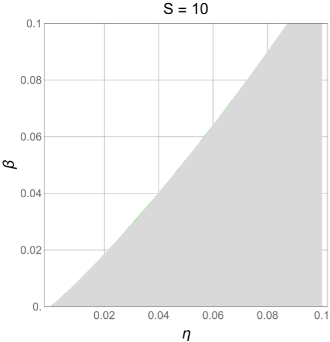
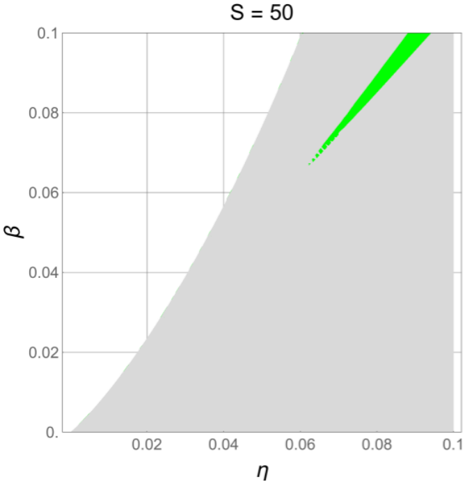
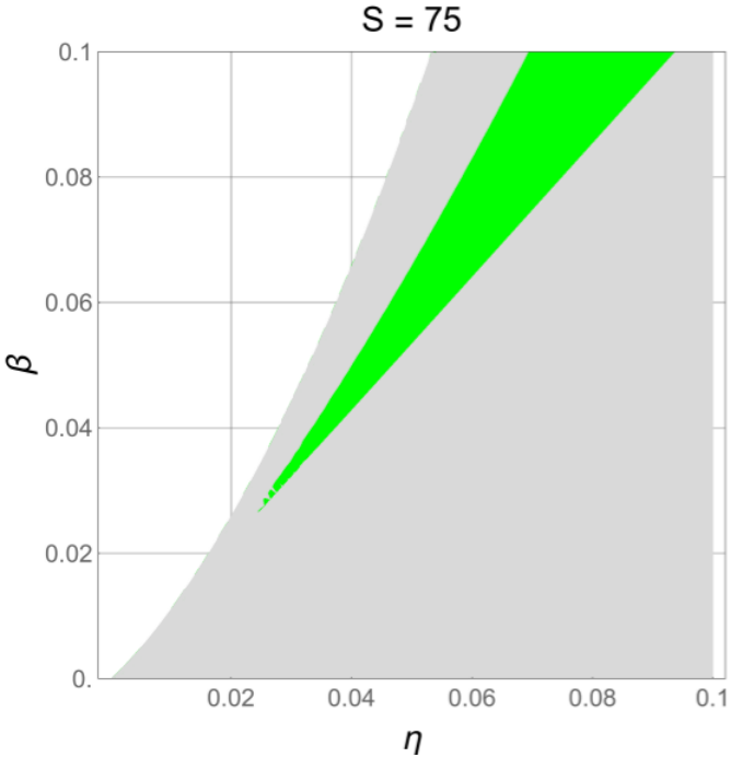
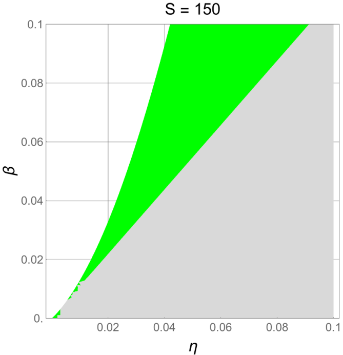
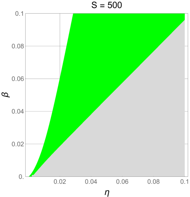
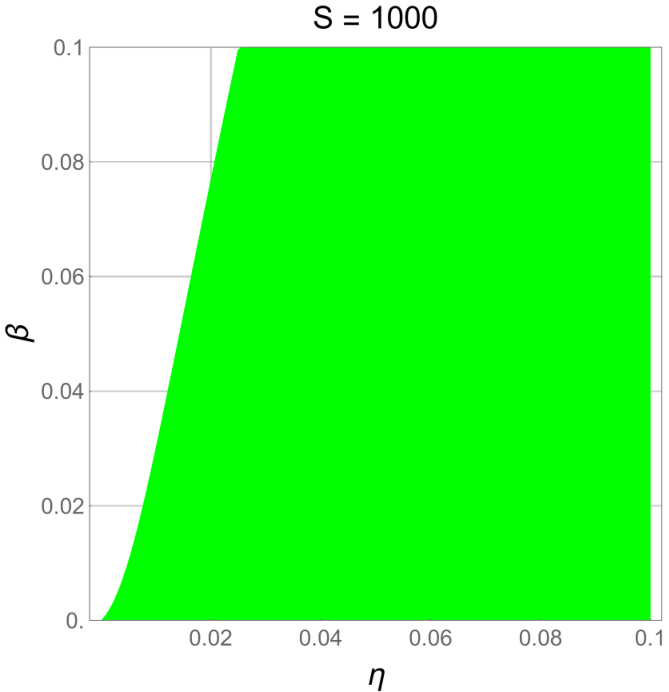
Now we explore the dependence of the coexistence solution and its stability in terms of the parameters $\eta$ and $\beta$ which describe the effects of the toxin on the strains. Figure 3 shows the regions at which the coexistence solution is stable, here represented by the green area. The gray region represents the set of the parameter space at which the solution still makes sense though it is not stable. In the graph the dependence of the stability region on the amount of resource is studied. Interestingly, we observe that the stability region grows as the resource influx rate $S$ increases. This is a quite striking outcome since in the absence of the toxin, the increase of the amount of resource available to the system favours the fixation of the selfish strain $D$ , while harsh envorinmental conditions tends to favour the cooperative trait [10, 7, 25]. This outcome evinces the role played by the toxin production as the coexistence is even enhanced as the resource becomes more abundant, thus warranting the maintenance of the efficient strain. In Figure 4 we see a heat map of the fraction and size of the population of both strains in terms of $\beta$ and $\eta$ in the set of parameters at which coexistence solution is stable. As expected, as $\eta$ is increased the fraction and size of the population of the strain $D$ is reduced. The same happening to the population of strain $C$ as $\beta$ rises. Although we also notice that, for fixed $\eta$ , an augment of $\beta$ favours the population of strain $D$ , the opposite situation, fixing $\beta$ and augmenting $\eta$ promotes a much higher variation in the population size of the efficient strain $C$ .

Conclusions

We have studied the possible solutions (extinction, only strain C, only strain D and coexistence) of a discrete-time model that describes the evolution of two competing metabolic strategies. The model assumes that the population is unstructured. One of the strains produces a toxin that affects the net growth rate of both strains, yet with different strength. As empirically found, the model predicts that the coexistence between a high yield strain and a high rate strain is possible. This outcome corroborates the fact that structuring is not the only possible mechanism promoting coexistence.

When the effect of the toxin on the efficient strain is negligible, the coexistence between the two strain types is possible for intermediate levels of the relative efficiency, $\Delta$ , of the inefficient strain. As expected, for very low values of $\Delta$ the efficient strain dominates while for high values of $\Delta$ the inefficient strain dominates. The novelty comes about with the observation of a coexistence regime which takes place at intermediate values of $\Delta$ , which is lacking if the toxin is not considered [24].

In the following we explored a more general scenario in which the toxin also attenuates the growth rate of the efficient strain. At this point, the analysis relied on values of relative efficiency $\Delta$ at which the cooperative strain is not favored in the absence of toxin, and extensively probed the outcome of the model in the parameter space $\eta$ vs $\beta$ . A striking finding of the model is the observation that the resource influx rate has a prominent role in driving the fate of the population. In a situation where the resource is scarce the population evolves to a pure population of only individuals of type $D$ (inefficient strain) and the coexistence solution is always unstable. However, as the resource influx rate rises a coexistence domain emerges. The domain of the coexistence solution starts just after the pure strain $D$ solution becomes unstable and widens out as the resource influx rate is augmented. This is quite surprising as the plenty of resource usually favors the defecting behavior [25]. However, although a large amount of resource into the system means that the inefficient strain ends up seizing a large amount of resource and consequently has an immediate positive effect on the growth rate, subsequently it also enhances the production of byproducts (toxin).

Our results corroborates the empirical observation that the coexistence between competing metabolic strategies is a possible outcome, and proves the effectiveness of the metabolite intermediate as the main driving mechanism for this purpose. Counterintuitively, our results evince that this coexistence is enhanced in a scenario of plentiful of resource.

Acknowledgments

PRAC is partially supported by Conselho Nacional de Desenvolvimento Científico e Tecnológico (CNPq), and also acknowledges financial support from Fundação de Amparo à Ciência e Tecnologia do Estado de Pernambuco (FACEPE). FFF gratefully acknowledges financial support from FAPESP (Fundação de Amparo à Pesquisa do Estado de São Paulo). JL is supported by Fundação de Amparo à Ciência e Tecnologia do Estado de Pernambuco (FACEPE) and AA has a fellowship from Conselho Nacional de Desenvolvimento Científico e Tecnológico (CNPq).

Appendix A

The general form of the Jacobian matrix for the analytical approximation is a $2\times 2$ with entries

$\displaystyle J_{11}$	$\displaystyle=1-\nu+a_{D}\left\{1-\exp\left[-\alpha_{D}\frac{\epsilon S}{n_{C}(t)+\epsilon n_{D}(t)}\right]\left[1+\alpha_{D}S\frac{n_{D}(t)\epsilon^{2}}{[n_{C}(t)+\epsilon n_{D}(t)]^{2}}\right]\right\}-2\eta\,n_{D}(t)$	(28)
$\displaystyle J_{12}$	$\displaystyle=-n_{D}(t)\left\{a_{D}\alpha_{D}\,S\frac{\epsilon\exp\left[-\alpha_{D}\frac{\epsilon S}{n_{C}(t)+\epsilon n_{D}(t)}\right]}{[n_{C}(t)+\epsilon n_{D}(t)]^{2}}\right\}$	(29)
$\displaystyle J_{21}$	$\displaystyle=-n_{C}(t)\left\{a_{C}\alpha_{C}S\frac{\epsilon\exp\left[-\alpha_{C}\frac{S}{n_{C}(t)+\epsilon n_{D}(t)}\right]}{[n_{C}(t)+\epsilon n_{D}(t)]^{2}}+\beta\right\}$	(30)
$\displaystyle J_{22}$	$\displaystyle=1-\nu+a_{C}\left\{1-\exp{\left[-\alpha_{C}\frac{S}{n_{C}(t)+\epsilon n_{D}(t)}\right]}\left[1+\alpha_{C}S\frac{n_{C}(t)}{[n_{C}(t)+\epsilon n_{D}(t)]^{2}}\right]\right\}-\beta\,n_{D}(t)$	(31)

References

[1] R.A. Fisher, The Genetical Theory of Natural Selection, Oxford University Press (1930)
[2] J.B. Haldane, A Mathematical Theory of Natural and Artificial Selection, Proceedings of the Cambridge Philosophical Society 23, 838 (1927).
[3] S. Wright, Evolution in mendelian populations, Genetics 16, 27 (1931).
[4] W.D. Hamilton, J. Theor. Biol. 7, 1 (1964)
[5] R.M. Axelrod, The evolution of cooperation, Basic Books (1984).
[6] P. C. J. Donoghue, J.B. Antcliffe, Nature 466, 41 (2010).
[7] T. Frick, S. Schuster, Naturwissenchaften 90, 327 (2003).
[8] P. E. Turner, L. Chao, Nature 398, 441 (1999).
[9] C. Hauert and L. Imhof, J. Theor. Biol 299, 106 (2012).
[10] T. Pfeiffer, S. Schuster and S. Bonhoeffer, Science 292, 504 (2001).
[11] T. Pfeiffer and S. Schuster, Trends in biochemical sciences 30, 20 (2005).
[12] P. R. Rich, Biochemical Society Transactions, 31, 1095 (2003).
[13] R.B. Helling, Journal of bacteriology, 184, 1041 (2002).
[14] J.C. Aledo, J.A. Pérez-Claros, A.E. del Valle, J Mol Evol 65, 328 (2007).
[15] R.C. MacLean, Heredity 100, 471 (2008).
[16] R.C. MacLean, I. Gudelj, Nature 44, 498 (2006).
[17] J.R. Meyer, I. Gudelj and R. Beardmore, Nature communications 6, 6278 (2015).
[18] O. Kappler, P.H. Janssen, J.-U. Kreft and B. Schink, Microbiology 143, 1105 (1997).
[19] K. Otterstedt, C. Larsson, R.M. Bill, A. Ståhlberg, E. Boles, S. Hohmann and L. Gustafsson, EMBO reports 5, 532(2004).
[20] M. Novak, T. Pfeiffer, R.E. Lenski, U. Sauer and S. Bonhoeffer, The American Naturalist 168, 242 (2006).
[21] D. A. Lipson, R. K. Monson, S.K. Schmidt and M.N. Weintraub, Biogeochemistry 95, 23 (2009).
[22] E. Postma, C. Verduyn, W.A. Scheffers and J.P. Van Dijken, Applied and environmental microbiology, 55, 468 (1989).
[23] G. Hardin, Science 162, 1243 (1968).
[24] A. Amado, L. Fernández, W. Huang, F.F. Ferreira, P.R.A. Campos, arXiv:1602.04773 [q-bio] (2016).
[25] F.F. Ferreira, P.R.A. Campos, Phys. Rev. E 88, 014101 (2013).