跳到论文正文
W Papers独立论文阅读器 arXiv:1606.05879 论文正文 计算阅读时间 · 0%
引用这篇论文根据当前论文元数据生成,正式投稿前建议核对。


License: arXiv.org perpetual non-exclusive license
arXiv:1606.05879v2 [gr-qc] 07 Sep 2016

UFIFT-QG-16-03

Precision Predictions for the Primordial Power Spectra
from f⁡(R)f(R) Models of Inflation

D. J. Brooker1∗, S. D. Odintsov2,3,4⋆ and R. P. Woodard1†

1 Department of Physics, University of Florida,
Gainesville, FL 32611, UNITED STATES

2 Institute of Space Sciences (IEEC-CSIC)
C. Can Magrans s/n, 08193 Barcelona, SPAIN

3 ICREA, Passeig Lluis Companys 23, 08010 Barcelona, SPAIN

4 INFN Sez. di Napoli, Compl. Univ. di Monte S. Angelo,
Edificio G, Via Cinthia, I-80126, Napoli, ITALY

ABSTRACT

We study the power spectra of f⁡(R)f(R) inflation using a new technique in which the norm-squared of the mode functions is evolved. Our technique results in excellent analytic approximations for how the spectra depend upon the function f⁡(R)f(R). Although the spectra are numerically the same in the Jordan and Einstein frames for the same wave number kk, they depend upon the geometries of these frames in quite different ways. For example, the power spectra in the two frames are different functions of the number of e-foldings until end of inflation. We discuss how future data on reheating can be used to distinguish f⁡(R)f(R) inflation from scalar-driven inflation.

PACS numbers: 04.50.Kd, 95.35.+d, 98.62.-g

∗ e-mail: djbrooker@ufl.edu

⋆ e-mail: odintsov@ieec.uab.es

† e-mail: woodard@phys.ufl.edu

1 Introduction

The proposal that the evolution of the universe is caused mainly by gravitation attracts more and more attention. However, it has been realized that gravity is not as simple as we thought and could be modified from standard General Relativity in several ways. Modified gravity theories are especially attractive to explain the current phase of cosmic acceleration.

The first complete model of primordial inflation was the 1980 proposal by Starobinsky to modify the gravitational Lagrangian by the addition of a term quadratic in the Ricci scalar [1]. Although this model was for decades eclipsed by scalar potential models, the increasingly tight bounds on the tensor-to-scalar ratio [2], and the consequent elimination of the simplest potentials [3], have combined to produce a resurgence of interest in it [4].

It has been realized lately that more general modifications of the Hilbert Lagrangian, from RR to f⁡(R)f(R), may provide a consistent description of late time acceleration [5, 6], or even provide a unified description of primordial inflation and dark energy [7]. A number of modified gravities which may consistently describe such a unified evolution of the universe are known [8, 9]. f⁡(R)f(R) gravity has attracted the main interest because it is ghost-free and reasonably simple.

It is quite remarkable that f⁡(R)f(R) gravity appears as a two-faced Janus: in the Jordan frame it is a modified gravity theory, whereas it is a kind of scalar-tensor theory after conformal transformation to the Einstein frame. The equivalence of the two frames has been demonstrated for some important observables [10, 11, 12, 13], however, that may not be the whole story for a number of reasons:

  • •

    Singularities (typical for super-acceleration) can lead to a breakdown of the mathematical equivalence between the two frames [14, 15, 16];

  • •

    The non-gravitational sector of the theory knows the difference because matter is minimally coupled in the Jordan frame whereas the coupling is highly non-minimal in the Einstein frame [17, 18]; and

  • •

    It can happen that the universe accelerates in one frame while decelerating in the other [19].

Nevertheless, it is expected that, for regular geometries, and in the absence of matter, the two frames are indeed equivalent. Studies of f⁡(R)f(R) inflation have been made in the Jordan frame [20, 21, 22, 23], but the normal, and much easier approach, is to work in the Einstein frame.

Although we shall have to discuss the issue of frame dependence somewhat, the purpose of this paper is to extend to f⁡(R)f(R) inflation a new formalism for computing the scalar and tensor power spectra. The formalism is based on first replacing the usual linear evolution equations for the mode functions with nonlinear evolution equations for the norm-squared mode functions which go into the power spectra [24]. This avoids the wasted effort of keeping track of the irrelevant phase. We then factor out the exact solutions which exist for constant first slow roll parameter, and derive a Green’s function solution for the residual factor [25, 26] which can be written for an arbitrary inflationary geometry. The power inherent is this analytic functional representation has been recently exploited to derive an improved version [27] of the famous single scalar consistency relation [28, 29, 30].

In section 2 we show how primordial perturbations appear in the Jordan and Einstein frames. Section 3 is devoted to the issue of using the power spectra (when the tensor power spectrum is eventually resolved) to reconstruct either a scalar potential model or an f⁡(R)f(R) model which would generate them. In section 4 we apply the new technique to two models of f⁡(R)f(R) inflation. Our conclusions comprise section 5.

2 Numerical Equality but Form Dependence

The purpose of this section is to show that the scalar and tensor perturbation fields of the Jordan and Einstein frames agree, but their power spectra nonetheless take highly different forms when expressed in terms of the geometrical quantities of each frame. We begin with a careful definition of the two frames, their backgrounds, their natural gauges and their perturbation fields. We then give the relation between the backgrounds and perturbations of each frame. The Starobinsky model provides a nice illustration of frame dependence because the standard slow roll approximations for the power spectra are valid in the Einstein frame but completely incorrect in the Jordan frame.

2.1 The Model in the Jordan Frame

The (spacelike) metric of the Jordan frame is gμ​νg_{\mu\nu}, which couples minimally to matter and gives physical distances and times. The Lagrangian of this frame is,

ℒ=f⁡(R)​−g16​π​G.\mathcal{L}=\frac{f(R)\sqrt{-g}}{16\pi G}\;. (1)

Its equation of motion is,

f′​(R)​Rμ​ν−12​f​(R)​gμ​ν+[gμ​ν​            −Dμ​Dν]​f′​(R)=0,f^{\prime}(R)R_{\mu\nu}-\frac{1}{2}f(R)g_{\mu\nu}+\Bigl[g_{\mu\nu}\kern 1.0pt\vbox{\hrule height=1.2pt\hbox{\vrule width=1.2pt\hskip 3.0pt\vbox{\vskip 6.0pt}\hskip 3.0pt\vrule width=0.6pt}\hrule height=0.6pt}\kern 1.0pt-D_{\mu}D_{\nu}\Bigr]f^{\prime}(R)=0\;, (2)

where DμD_{\mu} represents the covariant derivative operator and            ≡gμ​ν​Dμ​Dν\kern 1.0pt\vbox{\hrule height=1.2pt\hbox{\vrule width=1.2pt\hskip 3.0pt\vbox{\vskip 6.0pt}\hskip 3.0pt\vrule width=0.6pt}\hrule height=0.6pt}\kern 1.0pt\equiv g^{\mu\nu}D_{\mu}D_{\nu} is the covariant d’Alembertian.

The background geometry of the Jordan frame takes the form,

d​s2=−d​t2+a2​(t)​d​x→⋅d​x→=a2​(t)​[−d​η2+d​x→⋅d​x→].ds^{2}=-dt^{2}+a^{2}(t)d\vec{x}\!\cdot\!d\vec{x}=a^{2}(t)\Bigl[-d\eta^{2}+d\vec{x}\!\cdot\!d\vec{x}\Bigr]\;. (3)

One can see from (2) one can see that this background obeys the equations,

0\displaystyle 0 =\displaystyle\!\!\!=\!\!\! −3​(H˙+H2)​f′​(R0​(t))+12​f​(R0​(t))+3​H​∂tf′​(R0​(t)),\displaystyle-3(\dot{H}\!+\ H^{2})f^{\prime}\Bigl(R_{0}(t)\Bigr)+\frac{1}{2}f\Bigl(R_{0}(t)\Bigr)+3H\partial_{t}f^{\prime}\Bigl(R_{0}(t)\Bigr)\;, (4)
0\displaystyle 0 =\displaystyle\!\!\!=\!\!\! (H˙+3H2)f′(R0(t))−12f(R0(t))−(∂t2+2H∂t)f′(R0(t)).\displaystyle(\dot{H}\!+\!3H^{2})f^{\prime}\Bigl(R_{0}(t)\Bigr)-\frac{1}{2}f\Bigl(R_{0}(t)\Bigr)-(\partial_{t}^{2}\!+\!2H\partial_{t})f^{\prime}\Bigl(R_{0}(t)\Bigr)\;.\quad (5)

Here and henceforth H⁡(t)≡a˙/aH(t)\equiv\dot{a}/a is the Hubble parameter of the Jordan frame and R0​(t)≡6​H˙​(t)+12​H2​(t)R_{0}(t)\equiv 6\dot{H}(t)+12H^{2}(t) is the background value of the Ricci scalar. Adding (4) to (5) gives a relation we shall exploit later,

∂t[f′′​(R0)​R˙0]=−2​H˙​f′​(R0)+H​f′′​(R0)​R˙0.\partial_{t}\Bigl[f^{\prime\prime}(R_{0})\dot{R}_{0}\Bigr]=-2\dot{H}f^{\prime}(R_{0})+Hf^{\prime\prime}(R_{0})\dot{R}_{0}\;. (6)

The natural temporal gauge condition for the Jordan frame is R⁡(t,x→)=R0​(t)R(t,\vec{x})=R_{0}(t) [31]. In this gauge the g00g_{00} and g0​ig_{0i} components of the metric are constrained fields. The gi​jg_{ij} components take the form,

gi​j​(t,x→)=a2​(t)×e2​ζ​(t,x→)×[eh⁡(t,x→)]i​j,hi​i​(t,x→)=0.g_{ij}(t,\vec{x})=a^{2}(t)\times e^{2\zeta(t,\vec{x})}\times\Bigl[e^{h(t,\vec{x})}\Bigr]_{ij}\qquad,\qquad h_{ii}(t,\vec{x})=0\;. (7)

Note that requiring hi​i=0h_{ii}=0 is not a gauge condition but rather how one defines the breakup between ζ\zeta and hi​jh_{ij}. The spatial gauge condition is,

∂ihi​j​(t,x→)=0.\partial_{i}h_{ij}(t,\vec{x})=0\;. (8)

The homogeneity and isotropy of the Jordan frame background implies that the perturbation fields have the following free field expansions,

hi​j​(t,x→)\displaystyle h_{ij}(t,\vec{x}) =\displaystyle= 32​π​G∫d3​k(2​π)3∑λ=±{u(t,k)ei​k→⋅x→ϵi​j(k→,λ)α(k→,λ)+c.c.},\displaystyle\sqrt{32\pi G}\int\!\!\frac{d^{3}k}{(2\pi)^{3}}\sum_{\lambda=\pm}\Biggl\{u(t,k)e^{i\vec{k}\cdot\vec{x}}\epsilon_{ij}(\vec{k},\lambda)\alpha(\vec{k},\lambda)+{\rm c.c.}\Biggr\}\;,\qquad (9)
ζ⁡(t,x→)\displaystyle\zeta(t,\vec{x}) =\displaystyle= 4​π​G∫d3​k(2​π)3{v(t,k)ei​k→⋅x→β(k→)+c.c.}.\displaystyle\sqrt{4\pi G}\int\!\!\frac{d^{3}k}{(2\pi)^{3}}\Biggl\{v(t,k)e^{i\vec{k}\cdot\vec{x}}\beta(\vec{k})+{\rm c.c.}\Biggr\}\;. (10)

The polarization tensor ϵi​j​(k→,λ)\epsilon_{ij}(\vec{k},\lambda) obeys the same relations as in flat space, and is identical to the flat space result,

ki​ϵi​j=0=ϵi​i,ϵi​j​(k→,κ)​ϵi​j∗​(k→,λ)=δκ​λ.k_{i}\epsilon_{ij}=0=\epsilon_{ii}\qquad,\qquad\epsilon_{ij}(\vec{k},\kappa)\epsilon^{*}_{ij}(\vec{k},\lambda)=\delta_{\kappa\lambda}\;. (11)

The creation and annihilation operators also obey the flat space relations,

[α⁡(k→,κ),α†​(p→,λ)]=δκ​λ​(2​π)3​δ3​(k→−p→),[β⁡(k→),β†​(p→)]=(2​π)3​δ3​(k→−p→).\Bigl[\alpha(\vec{k},\kappa),\alpha^{\dagger}(\vec{p},\lambda)\Bigr]=\delta_{\kappa\lambda}(2\pi)^{3}\delta^{3}(\vec{k}\!-\!\vec{p})\quad,\quad\Bigl[\beta(\vec{k}),\beta^{\dagger}(\vec{p})\Bigr]=(2\pi)^{3}\delta^{3}(\vec{k}\!-\!\vec{p})\;. (12)

It is best to define the (tree order) power spectra as the asymptotic late time forms of equal-time correlators,

Δh2​(t,k)\displaystyle\Delta^{2}_{h}(t,k) ≡\displaystyle\!\!\!\!\equiv\!\!\!\! k32​π2∫d3xe−ik→⋅x→⟨Ω|hi​j(t,x→)hi​j(t,0→)|Ω⟩\displaystyle\frac{k^{3}}{2\pi^{2}}\!\int\!\!d^{3}x\,e^{-i\vec{k}\cdot\vec{x}}\Bigl\langle\Omega\Bigl|h_{ij}(t,\vec{x})h_{ij}(t,\vec{0})\Bigr|\Omega\Bigr\rangle (13)
=k32​π2×32πG××|u(t,k)|2,\displaystyle\hskip 142.26378pt=\frac{k^{3}}{2\pi^{2}}\!\times\!32\pi G\!\times\!2\!\times\!|u(t,k)|^{2}\;,
Δℛ2​(t,k)\displaystyle\Delta^{2}_{\mathcal{R}}(t,k) ≡\displaystyle\!\!\!\!\equiv\!\!\!\! k32​π2∫d3xe−ik→⋅x→⟨Ω|ζ(t,x→)ζ(t,0→)|Ω⟩=k32​π2×4πG×|v(t,k)|2,\displaystyle\frac{k^{3}}{2\pi^{2}}\!\int\!\!d^{3}x\,e^{-i\vec{k}\cdot\vec{x}}\Bigl\langle\Omega\Bigl|\zeta(t,\vec{x})\zeta(t,\vec{0})\Bigr|\Omega\Bigr\rangle=\frac{k^{3}}{2\pi^{2}}\!\times\!4\pi G\!\times\!|v(t,k)|^{2}\;,\qquad (14)

The equations obeyed by the tensor mode function u⁡(t,k)u(t,k) are fairly easy to read off by linearizing (2) and applying canonical quantization,

u¨+(3​H+f′′​(R0)​R˙0f′​(R0))​u˙+k2a2​u=0,u​u˙∗−u˙​u∗=if′​(R0)​a3.\ddot{u}+\Bigl(3H\!+\!\frac{f^{\prime\prime}(R_{0})\dot{R}_{0}}{f^{\prime}(R_{0})}\Bigr)\dot{u}+\frac{k^{2}}{a^{2}}\,u=0\qquad,\qquad u\dot{u}^{*}-\dot{u}u^{*}=\frac{i}{f^{\prime}(R_{0})a^{3}}\;. (15)

Obtaining the scalar mode equations is much more difficult because one must first solve the constraints. A long calculation reveals that v⁡(t,k)v(t,k) obeys,

v¨+(3​H+f′′​(R0)​R˙0f′​(R0)+E˙E)​v˙+k2a2​v=0,v​v˙∗−v˙​v∗=iE​f′​(R0)​a3,\ddot{v}+\Bigl(3H\!+\!\frac{f^{\prime\prime}(R_{0})\dot{R}_{0}}{f^{\prime}(R_{0})}\!+\!\frac{\dot{E}}{E}\Bigr)\dot{v}+\frac{k^{2}}{a^{2}}\,v=0\quad,\quad v\dot{v}^{*}-\dot{v}v^{*}=\frac{i}{Ef^{\prime}(R_{0})a^{3}}\;, (16)

where the function E⁡(t)E(t) is,

E=3​(f′′​(R0)​R˙02​f′​(R0)​H)2(+f′′​(R0)​R˙02​f′​(R0)​H)2.E=\frac{3(\frac{f^{\prime\prime}(R_{0})\dot{R}_{0}}{2f^{\prime}(R_{0})H})^{2}}{(1\!+\!\frac{f^{\prime\prime}(R_{0})\dot{R}_{0}}{2f^{\prime}(R_{0})H})^{2}}\;. (17)

Differential equations such as (15-16) define the mode functions up to initial conditions. The usual (Bunch-Davies-like) initial conditions are that the WKB forms apply in the distant past,

u⁡(t,k)\displaystyle u(t,k) ⟶\displaystyle\longrightarrow 12​k​f′​(R0​(t))​a2​(t)exp[−ik∫titd​t′a⁡(t′)],\displaystyle\frac{1}{\sqrt{2kf^{\prime}(R_{0}(t))a^{2}(t)}}\,\exp\Bigl[-ik\!\int_{t_{i}}^{t}\!\frac{dt^{\prime}}{a(t^{\prime})}\Bigr]\;, (18)
v⁡(t,k)\displaystyle v(t,k) ⟶\displaystyle\longrightarrow 12​k​E​(t)​f′​(R0​(t))​a2​(t)exp[−ik∫titd​t′a⁡(t′)].\displaystyle\frac{1}{\sqrt{2kE(t)f^{\prime}(R_{0}(t))a^{2}(t)}}\,\exp\Bigl[-ik\!\int_{t_{i}}^{t}\!\frac{dt^{\prime}}{a(t^{\prime})}\Bigr]\;. (19)

One can see from (15-16) that the mode functions must approach constants when the term k2/a2​(t)k^{2}/a^{2}(t) becomes insignificant. Those constants can be found by using (15-16) to evolve u⁡(t,k)u(t,k) and v⁡(t,k)v(t,k) from their initial forms (18-19). Substituting those constants into the time-dependent power spectra (13-14) gives the model’s predictions for the primordial power spectra.

2.2 The Model in the Einstein Frame

The transformation from the Jordan frame to the Einstein frame is effected by first introducing an auxiliary scalar ϕ\phi which obeys the equation,

ϕ=f′(R)⟺R=ℛ(ϕ).\phi=f^{\prime}(R)\qquad\Longleftrightarrow\qquad R=\mathcal{R}(\phi)\;. (20)

We then construct a potential U⁡(ϕ)U(\phi) by Legendre transforming,

U(ϕ)≡ϕℛ(ϕ)−f(ℛ(ϕ))⟺U′(ϕ)=ℛ(ϕ).U(\phi)\equiv\phi\mathcal{R}(\phi)-f\Bigl(\mathcal{R}(\phi)\Bigr)\qquad\Longleftrightarrow\qquad U^{\prime}(\phi)=\mathcal{R}(\phi)\;. (21)

The Einstein frame Lagrangian is,

ℒ~=116​π​G​[ϕ​R−U​(ϕ)]​−g.\widetilde{\mathcal{L}}=\frac{1}{16\pi G}\Bigl[\phi R-U(\phi)\Bigr]\sqrt{-g}\;. (22)

The two field equations associated with (22) are,

0\displaystyle 0 =\displaystyle= R−U′​(ϕ),\displaystyle R-U^{\prime}(\phi)\;, (23)
0\displaystyle 0 =\displaystyle= ϕ​Rμ​ν−12​[ϕ​R−U⁡(ϕ)]+[gμ​ν​            −Dμ​Dν]​ϕ.\displaystyle\phi R_{\mu\nu}-\frac{1}{2}\Bigl[\phi R\!-\!U(\phi)\Bigr]+\Bigl[g_{\mu\nu}\kern 1.0pt\vbox{\hrule height=1.2pt\hbox{\vrule width=1.2pt\hskip 3.0pt\vbox{\vskip 6.0pt}\hskip 3.0pt\vrule width=0.6pt}\hrule height=0.6pt}\kern 1.0pt\!-\!D_{\mu}D_{\nu}\Bigr]\phi\;. (24)

Of course (23) reproduces (20), whereupon we recognize (24) as the Jordan frame equation (2).

We reach the final form of the Einstein frame by making a field redefinition which is the conformal transformation,

g~μ​ν≡ϕ​gμ​ν\displaystyle\widetilde{g}_{\mu\nu}\equiv\phi g_{\mu\nu}\qquad ⟺\displaystyle\Longleftrightarrow gμ​ν=exp⁡[−16​π​G3​φ]​g~μ​ν,\displaystyle\qquad g_{\mu\nu}=\exp\Biggl[-\sqrt{\frac{16\pi G}{3}}\,\varphi\Biggr]\widetilde{g}_{\mu\nu}\;, (25)
φ≡316​π​G​ln⁡(ϕ)\displaystyle\varphi\equiv\sqrt{\frac{3}{16\pi G}}\,\ln(\phi)\qquad ⟺\displaystyle\Longleftrightarrow ϕ=exp⁡[16​π​G3​φ].\displaystyle\qquad\phi=\exp\Biggl[\sqrt{\frac{16\pi G}{3}}\,\varphi\Biggr]\;. (26)

Substituting (25-26) in (22) gives the classic form of a minimally coupled scalar,

ℒ~=R~​−g~16​π​G−12​∂μφ​∂νφ​g~μ​ν​−g~−V⁡(φ)​−g~.\widetilde{\mathcal{L}}=\frac{\widetilde{R}\sqrt{-\widetilde{g}}}{16\pi G}-\frac{1}{2}\partial_{\mu}\varphi\partial_{\nu}\varphi\widetilde{g}^{\mu\nu}\sqrt{-\widetilde{g}}-V(\varphi)\sqrt{-\widetilde{g}}\;. (27)

where the scalar potential is,

V⁡(φ)≡116​π​G​exp⁡[−2​16​π​G3​φ]​U​(exp⁡[16​π​G3​φ]).V(\varphi)\equiv\frac{1}{16\pi G}\,\exp\Biggl[-2\sqrt{\frac{16\pi G}{3}}\,\varphi\Biggr]U\Biggl(\exp\Biggl[\sqrt{\frac{16\pi G}{3}}\,\varphi\Biggr]\Biggr)\;. (28)

The background geometry of the Einstein frame takes the form,

d​s~2=−d​t~2+a~2​(t~)​d​x→⋅d​x→=a~2​(t~)​[−d​η2+d​x→⋅d​x→].d\widetilde{s}^{2}=-d\widetilde{t}^{2}+\widetilde{a}^{2}(\widetilde{t})d\vec{x}\!\cdot\!d\vec{x}=\widetilde{a}^{2}(\widetilde{t})\Bigl[-d\eta^{2}+d\vec{x}\!\cdot\!d\vec{x}\Bigr]\;. (29)

It relates to the background scalar field φ0​(t~)\varphi_{0}(\widetilde{t}) through the Einstein equations,

3​H~2​(t~)\displaystyle 3\widetilde{H}^{2}(\widetilde{t}) =\displaystyle= 8​π​G​[12​φ˙02​(t~)+V⁡(φ0​(t~))],\displaystyle 8\pi G\Bigl[\frac{1}{2}\dot{\varphi}_{0}^{2}(\widetilde{t})+V\Bigl(\varphi_{0}(\widetilde{t})\Bigr)\Bigr]\;, (30)
−2​H~˙​(t~)−3​H~2​(t~)\displaystyle-2\dot{\widetilde{H}}(\widetilde{t})-3\widetilde{H}^{2}(\widetilde{t}) =\displaystyle= 8​π​G​[12​φ˙02​(t~)−V⁡(φ0​(t~))].\displaystyle 8\pi G\Bigl[\frac{1}{2}\dot{\varphi}_{0}^{2}(\widetilde{t})-V\Bigl(\varphi_{0}(\widetilde{t})\Bigr)\Bigr]\;. (31)

The natural temporal gauge condition in the Einstein frame is φ⁡(t~,x→)=φ0​(t~)\varphi(\widetilde{t},\vec{x})=\varphi_{0}(\widetilde{t}) [32]. In this gauge the g~00\widetilde{g}_{00} and g~0​i\widetilde{g}_{0i} components of the metric are constrained fields and the spatial components take the form,

g~i​j​(t~,x→)≡a~2​(t~)×e2​ζ~​(t~,x→)×[eh~​(t~,x→)]i​j,h~i​i=0.\widetilde{g}_{ij}(\widetilde{t},\vec{x})\equiv\widetilde{a}^{2}(\widetilde{t})\times e^{2\widetilde{\zeta}(\widetilde{t},\vec{x})}\times\Bigl[e^{\widetilde{h}(\widetilde{t},\vec{x})}\Bigr]_{ij}\qquad,\qquad\widetilde{h}_{ii}=0\;. (32)

Note that requiring h~i​j​(t~,x→)\widetilde{h}_{ij}(\widetilde{t},\vec{x}) to be traceless is not a gauge condition but rather part of the definition of ζ~​(t~,x→)\widetilde{\zeta}(\widetilde{t},\vec{x}). The true spatial gauge condition is the transversality of h~i​j​(t~,x→)\widetilde{h}_{ij}(\widetilde{t},\vec{x}),

∂ih~i​j​(t~,x→)=0.\partial_{i}\widetilde{h}_{ij}(\widetilde{t},\vec{x})=0\;. (33)

Homogeneity and isotropy are also symmetries in the Einstein frame so we can expand the perturbation fields the same way as in the Jordan frame, only with different mode functions,

h~i​j​(t~,x→)\displaystyle\widetilde{h}_{ij}(\widetilde{t},\vec{x}) =\displaystyle= 32​π​G∫d3​k(2​π)3∑λ=±{u~(t~,k)ei​k→⋅x→ϵi​j(k→,λ)α(k→,λ)+c.c.},\displaystyle\sqrt{32\pi G}\int\!\!\frac{d^{3}k}{(2\pi)^{3}}\sum_{\lambda=\pm}\Biggl\{\widetilde{u}(\widetilde{t},k)e^{i\vec{k}\cdot\vec{x}}\epsilon_{ij}(\vec{k},\lambda)\alpha(\vec{k},\lambda)+{\rm c.c.}\Biggr\}\;,\qquad (34)
ζ~​(t~,x→)\displaystyle\widetilde{\zeta}(\widetilde{t},\vec{x}) =\displaystyle= 4​π​G∫d3​k(2​π)3{v~(t~,k)ei​k→⋅x→β(k→)+c.c.}.\displaystyle\sqrt{4\pi G}\int\!\!\frac{d^{3}k}{(2\pi)^{3}}\Biggl\{\widetilde{v}(\widetilde{t},k)e^{i\vec{k}\cdot\vec{x}}\beta(\vec{k})+{\rm c.c.}\Biggr\}\;. (35)

Note that the polarization tensor of the Einstein frame is identical to that of the Jordan frame, as are the creation and annihilation operators. The time dependent power spectra are defined in the same way as for the Jordan frame to give,

Δ~h2​(t~,k)\displaystyle\widetilde{\Delta}^{2}_{h}(\widetilde{t},k) ≡\displaystyle\equiv k32​π2×32πG××|u~(t~,k)|2,\displaystyle\frac{k^{3}}{2\pi^{2}}\!\times\!32\pi G\!\times\!2\!\times\!|\widetilde{u}(\widetilde{t},k)|^{2}\;, (36)
Δ~ℛ2​(t~,k)\displaystyle\widetilde{\Delta}^{2}_{\mathcal{R}}(\widetilde{t},k) ≡\displaystyle\equiv k32​π2×4​π​G×|v~​(t~,k)|2.\displaystyle\frac{k^{3}}{2\pi^{2}}\!\times\!4\pi G\!\times\!|\widetilde{v}(\widetilde{t},k)|^{2}\;. (37)

By solving the constraint equations and employing canonical quantization one finds that the mode functions obey the following equations and Wronskian normalization conditions,

[∂2∂t~2+3​H~​∂∂t~+k2a~2]​u~=0\displaystyle\Bigl[\frac{\partial^{2}}{\partial\widetilde{t}^{2}}+3\widetilde{H}\frac{\partial}{\partial\widetilde{t}}+\frac{k^{2}}{\widetilde{a}^{2}}\Bigr]\widetilde{u}=0\qquad , u~​∂u~∗∂t~−∂u~∂t~​u~∗=ia~3,\displaystyle\qquad\widetilde{u}\frac{\partial\widetilde{u}^{*}}{\partial\widetilde{t}}-\frac{\partial\widetilde{u}}{\partial\widetilde{t}}\,\widetilde{u}^{*}=\frac{i}{\widetilde{a}^{3}}\;, (38)
[∂2∂t~2+(3​H~+1ϵ~​d​ϵ~d​t~)​∂∂t~+k2a~2]​v~=0\displaystyle\Bigl[\frac{\partial^{2}}{\partial\widetilde{t}^{2}}+\Bigl(3\widetilde{H}\!+\!\frac{1}{\widetilde{\epsilon}}\frac{d\widetilde{\epsilon}}{d\widetilde{t}}\Bigr)\frac{\partial}{\partial\widetilde{t}}+\frac{k^{2}}{\widetilde{a}^{2}}\Bigr]\widetilde{v}=0\qquad , v~​∂v~∗∂t~−∂v~∂t~​v~∗=iϵ~​a~3.\displaystyle\qquad\widetilde{v}\frac{\partial\widetilde{v}^{*}}{\partial\widetilde{t}}-\frac{\partial\widetilde{v}}{\partial\widetilde{t}}\,\widetilde{v}^{*}=\frac{i}{\widetilde{\epsilon}\widetilde{a}^{3}}\;.\qquad (39)

The assumption of Bunch-Davies-like vacuum corresponds to the following asymptotic early time forms,

u~​(t~,k)\displaystyle\widetilde{u}(\widetilde{t},k) ⟶\displaystyle\longrightarrow 12​k​a~2​(t~)exp[−ik∫t~it~d​t′a~​(t′)],\displaystyle\frac{1}{\sqrt{2k\widetilde{a}^{2}(\widetilde{t})}}\,\exp\Bigl[-ik\!\int_{\widetilde{t}_{i}}^{\widetilde{t}}\!\frac{dt^{\prime}}{\widetilde{a}(t^{\prime})}\Bigr]\;, (40)
v~​(t~,k)\displaystyle\widetilde{v}(\widetilde{t},k) ⟶\displaystyle\longrightarrow 12​k​ϵ~​(t~)​a~2​(t~)exp[−ik∫t~it~d​t′a~​(t′)].\displaystyle\frac{1}{\sqrt{2k\widetilde{\epsilon}(\widetilde{t})\widetilde{a}^{2}(\widetilde{t})}}\,\exp\Bigl[-ik\!\int_{\widetilde{t}_{i}}^{\widetilde{t}}\!\frac{dt^{\prime}}{\widetilde{a}(t^{\prime})}\Bigr]\;. (41)

The model’s predictions for the primordial power spectra are obtained by using (38-39) to evolve u~​(t~,k)\widetilde{u}(\widetilde{t},k) and v~​(t~,k)\widetilde{v}(\widetilde{t},k) from their initial forms (40-41) to find their late time constant values, and then substituting these constants into the time dependent power spectra (36)-37).

2.3 Relating Backgrounds and Perturbation Fields

Comparison of expression (7) with (32), and relations (25-26), implies that the perturbation fields agree between the two frames [13],

ζ⁡(t,x→)\displaystyle\zeta(t,\vec{x}) =\displaystyle= ζ~​(t~,x→),\displaystyle\widetilde{\zeta}(\widetilde{t},\vec{x})\;, (42)
hi​j​(t,x→)\displaystyle h_{ij}(t,\vec{x}) =\displaystyle= h~i​j​(t~,x→).\displaystyle\widetilde{h}_{ij}(\widetilde{t},\vec{x})\;. (43)

This means that the scalar and tensor power spectra also agree numerically between the two frames. However, expressions for those power spectra are quite frame dependent because the expansion histories and co-moving times of the two frames do not agree,

a⁡(t)=exp⁡[−4​π​G3​φ​(t~)]×a~​(t~)\displaystyle a(t)=\exp\Bigl[-\sqrt{\frac{4\pi G}{3}}\,\varphi(\widetilde{t})\Bigr]\!\times\!\widetilde{a}(\widetilde{t})\;\; ⟺\displaystyle\Longleftrightarrow a~​(t~)=f′​(R0​(t))×a​(t),\displaystyle\;\;\widetilde{a}(\widetilde{t})=\sqrt{f^{\prime}\Bigl(R_{0}(t)\Bigr)}\!\times\!a(t)\;,\quad (44)
d​t=exp⁡[−4​π​G3​φ​(t~)]×d​t~\displaystyle dt=\exp\Bigl[-\sqrt{\frac{4\pi G}{3}}\,\varphi(\widetilde{t})\Bigr]\!\times\!d\widetilde{t}\;\; ⟺\displaystyle\Longleftrightarrow d​t~=f′​(R0​(t))×d​t.\displaystyle\;\;d\widetilde{t}=\sqrt{f^{\prime}\Bigl(R_{0}(t)\Bigr)}\!\times\!dt\;.\quad (45)

It follows that the Hubble parameter of the Einstein frame is,

H~​(t~)\displaystyle\widetilde{H}(\widetilde{t}) ≡\displaystyle\equiv dd​t~​ln⁡[a~​(t~)]=1f′​(R0​(t))​dd​t​ln⁡[f′​(R0​(t))​a​(t)],\displaystyle\frac{d}{d\widetilde{t}}\ln\Bigl[\widetilde{a}(\widetilde{t})\Bigr]=\frac{1}{\sqrt{f^{\prime}(R_{0}(t))}}\frac{d}{dt}\ln\Bigl[\sqrt{f^{\prime}(R_{0}(t))}\,a(t)\Bigr]\;,\qquad (46)
=\displaystyle= Hf′​(R0)​[1+f′′​(R0)​R˙02​f′​(R0)​H].\displaystyle\frac{H}{\sqrt{f^{\prime}(R_{0})}}\Biggl[1+\frac{f^{\prime\prime}(R_{0})\dot{R}_{0}}{2f^{\prime}(R_{0})H}\Biggr]\;. (47)

Using relation (6) the first slow roll parameter is,

ϵ~​(t~)≡dd​t~​1H~​(t~)=1f′​(R0)​dd​t​[f′​(R0)H+f′′​(R0)​R˙02​f′​(R0)]=3​(f′′​(R0)​R˙02​f′​(R0)​H)2[1+f′′​(R0)​R˙02​f′​(R0)​H]2.\widetilde{\epsilon}(\widetilde{t})\equiv\frac{d}{d\widetilde{t}}\frac{1}{\widetilde{H}(\widetilde{t})}=\frac{1}{\sqrt{f^{\prime}(R_{0})}}\frac{d}{dt}\Biggl[\frac{\sqrt{f^{\prime}(R_{0})}}{H+\frac{f^{\prime\prime}(R_{0})\dot{R}_{0}}{2f^{\prime}(R_{0})}}\Biggr]=\frac{3(\frac{f^{\prime\prime}(R_{0})\dot{R}_{0}}{2f^{\prime}(R_{0})H})^{2}}{[1+\frac{f^{\prime\prime}(R_{0})\dot{R}_{0}}{2f^{\prime}(R_{0})H}]^{2}}\;. (48)

Both parameters depend critically on the function XX,

X≡f′′​(R0)​R˙02​f′​(R0)​H=−f′′​(R0)​R0f′​(R0)​[ϵ+ϵ˙2​(−ϵ)​H],X\equiv\frac{f^{\prime\prime}(R_{0})\dot{R}_{0}}{2f^{\prime}(R_{0})H}=-\frac{f^{\prime\prime}(R_{0})R_{0}}{f^{\prime}(R_{0})}\Bigl[\epsilon+\frac{\dot{\epsilon}}{2(2\!-\!\epsilon)H}\Bigr]\;, (49)

where the final form on the right follows from R0=6​(2−ϵ)​H2R_{0}=6(2-\epsilon)H^{2} and hence,

R˙0=−12​ϵ​(−ϵ)​H3−6​ϵ˙​H2=−2​H​(ϵ​R0+3​ϵ˙​H).\dot{R}_{0}=-12\epsilon(2\!-\!\epsilon)H^{3}-6\dot{\epsilon}H^{2}=-2H(\epsilon R_{0}\!+\!3\dot{\epsilon}H)\;. (50)

Combining relations (47-48) with the usual slow roll results for the power spectra in the Einstein frame (and hence also in the Jordan frame) gives,

Δℛ2​(k)≃G​H~2π​ϵ~\displaystyle\Delta^{2}_{\mathcal{R}}(k)\simeq\frac{G\widetilde{H}^{2}}{\pi\widetilde{\epsilon}} =\displaystyle= G​H2​(+X)43​π​f′​(R0)​X2,\displaystyle\frac{GH^{2}(1\!+\!X)^{4}}{3\pi f^{\prime}(R_{0})X^{2}}\;, (51)
Δh2​(k)≃16π​G​H~2\displaystyle\Delta^{2}_{h}(k)\simeq\frac{16}{\pi}G\widetilde{H}^{2} =\displaystyle= 16​G​H2​(+X)2π​f′​(R0).\displaystyle\frac{16GH^{2}(1\!+\!X)^{2}}{\pi f^{\prime}(R_{0})}\;. (52)

Therefore, the tensor-to-scalar ratio is,

r⁡(k)≡Δh2​(k)Δℛ2​(k)≈16​ϵ~=48​X2(+X)2.r(k)\equiv\frac{\Delta^{2}_{h}(k)}{\Delta^{2}_{\mathcal{R}}(k)}\approx 16\widetilde{\epsilon}=\frac{48X^{2}}{(1\!+\!X)^{2}}\;. (53)

Successful models of f⁡(R)f(R) inflation typically have f′′​(R0)​R0/f′​(R0)∼1f^{\prime\prime}(R_{0})R_{0}/f^{\prime}(R_{0})\sim 1, so relation (49) implies X∼−ϵX\sim-\epsilon. Substituting into relation (53) means that slow roll inflation in the Einstein frame, with r≈16​ϵ~r\approx 16\widetilde{\epsilon}, typically implies r≈48​ϵ2r\approx 48\epsilon^{2} when expressed using the Jordan frame geometry.

2.4 Starobinsky Inflation

Starobinsky inflation corresponds to,

f⁡(R)=R+8​π​G​R26​M2⟹f′​(R)=1+16​π​G​R6​M2⟹f′′​(R)=16​π​G6​M2.f(R)=R+\frac{8\pi GR^{2}}{6M^{2}}\quad\Longrightarrow\quad f^{\prime}(R)=1+\frac{16\pi GR}{6M^{2}}\quad\Longrightarrow\quad f^{\prime\prime}(R)=\frac{16\pi G}{6M^{2}}\;. (54)

Substituting (54) into the background equations (4-5) reveals a good approximate solution with,

H˙​(t)≃−M248​π​G≡−ϵi​Hi2,\dot{H}(t)\simeq-\frac{M^{2}}{48\pi G}\equiv-\epsilon_{i}H_{i}^{2}\;, (55)

where HiH_{i} and ϵi\epsilon_{i} are the initial values of the Hubble and first slow roll parameters. Hence the various geometrical parameters are,

ϵ⁡(t)\displaystyle\epsilon(t) ≃\displaystyle\simeq ϵi[−ϵi​Hi​Δ​t]2,\displaystyle\frac{\epsilon_{i}}{[1\!-\!\epsilon_{i}H_{i}\Delta t]^{2}}\;, (56)
H⁡(t)\displaystyle H(t) ≃\displaystyle\simeq Hi​[−ϵi​Hi​Δ​t],\displaystyle H_{i}[1\!-\!\epsilon_{i}H_{i}\Delta t]\;, (57)
a⁡(t)\displaystyle a(t) ≃\displaystyle\simeq ai​exp⁡[Hi​Δ​t−12​ϵi​(Hi​Δ​t)2].\displaystyle a_{i}\exp\Bigl[H_{i}\Delta t\!-\!\frac{1}{2}\epsilon_{i}(H_{i}\Delta t)^{2}\Bigr]\;. (58)

Expressing these parameters in terms of the number of e-foldings nn from the start of inflation gives,

ϵ=ϵi−2​ϵi​n,H=Hi​−2​ϵi​n,a=ai​en.\epsilon=\frac{\epsilon_{i}}{1\!-\!2\epsilon_{i}n}\quad,\quad H=H_{i}\sqrt{1\!-\!2\epsilon_{i}n}\quad,\quad a=a_{i}e^{n}\;. (59)

Under the usual assumption that 0<ϵi≪10<\epsilon_{i}\ll 1 we have,

f′′​(R0​(t))​R0​(t)≃23​ϵ​(t)≃f′​(R0​(t)).f^{\prime\prime}\Bigl(R_{0}(t)\Bigr)R_{0}(t)\simeq\frac{2}{3\epsilon(t)}\simeq f^{\prime}\Bigl(R_{0}(t)\Bigr)\;. (60)

Substituting into relation(49) implies,

X⁡(t)≃−ϵ⁡(t).X(t)\simeq-\epsilon(t)\;. (61)

Hence the first slow roll parameter of the Einstein frame (48) is much smaller than the first slow roll parameter of the Jordan frame, as depicted in Fig. 1. The power spectra and their ratio are,

Δℛ2​(k)\displaystyle\Delta^{2}_{\mathcal{R}}(k) ≃\displaystyle\simeq G​H22​π​ϵ≃G​Hi22​π​ϵi​[−2​ϵi​nk]2,\displaystyle\frac{GH^{2}}{2\pi\epsilon}\simeq\frac{GH_{i}^{2}}{2\pi\epsilon_{i}}\Bigl[1\!-\!2\epsilon_{i}n_{k}\Bigr]^{2}\;, (62)
Δh2​(k)\displaystyle\Delta^{2}_{h}(k) ≃\displaystyle\simeq 24π​G​H2​ϵ≃24π​G​Hi2​ϵi,\displaystyle\frac{24}{\pi}\,GH^{2}\epsilon\simeq\frac{24}{\pi}\,GH_{i}^{2}\epsilon_{i}\;, (63)
r⁡(k)\displaystyle r(k) ≃\displaystyle\simeq 48​ϵ2≃48​ϵi2(−2​ϵi​nk)2,\displaystyle 48\epsilon^{2}\simeq\frac{48\epsilon_{i}^{2}}{(1\!-\!2\epsilon_{i}n_{k})^{2}}\;, (64)

where nk≃ln⁡(k/ai​Hi)n_{k}\simeq\ln(k/a_{i}H_{i}) is the e-folding of first horizon crossing. This model actually obeys the famous single-scalar consistency relation [28, 29, 30] but one would need to carry the expansion of Δh2​(k)≃24π​G​H2​ϵ×(1−3​ϵ+…)\Delta^{2}_{h}(k)\simeq\frac{24}{\pi}GH^{2}\epsilon\times(1-3\epsilon+\dots) one more order to give a nonzero result for the tensor spectral index. However, relations (62-64) deviate extensively from the usual slow roll results when expressed in terms of the Jordan frame geometry.

Refer to caption
Figure 1: Comparison of first slow roll parameter in the two frames for Starobinsky inflation. The blue curve gives Jordan frame result ϵ\epsilon whereas the yellow curve shows the much smaller Einstein frame result ϵ~\widetilde{\epsilon} of expression (48).

Starobinsky inflation obeys the general rule of f⁡(R)f(R) inflation that its power spectra are numerically the same, for fixed wave number kk, in both Jordan and Einstein frames. However, what this “kk” means geometrically is very different in the two frames. One way to see the difference is by expressing the spectra in terms of the number of e-foldings until the end of inflation. From relation (44) we infer,

a~​(t~)≡a~i​en~≃a⁡(t)32​ϵ​(t)⟹a~i≃ai32​ϵi,n~≃n+12​ln⁡(−2​ϵi​n).\widetilde{a}(\widetilde{t})\equiv\widetilde{a}_{i}e^{\widetilde{n}}\simeq\frac{a(t)}{\sqrt{\frac{3}{2}\epsilon(t)}}\quad\Longrightarrow\quad\widetilde{a}_{i}\simeq\frac{a_{i}}{\sqrt{\frac{3}{2}\epsilon_{i}}}\;,\;\widetilde{n}\simeq n+\frac{1}{2}\ln(1\!-\!2\epsilon_{i}n)\;. (65)

Inflation ends at nend≃12​ϵi−12n_{\rm end}\simeq\frac{1}{2\epsilon_{i}}-\frac{1}{2}, which corresponds to n~end≃12​ϵi+12​ln⁡(ϵi)\widetilde{n}_{\rm end}\simeq\frac{1}{2\epsilon_{i}}+\frac{1}{2}\ln(\epsilon_{i}). The number of Jordan frame e-foldings until the end of inflation is N≡nend−nN\equiv n_{\rm end}-n, so the number of Einstein frame e-foldings until the end of inflation is,

N~≡n~end−n~≃N−12​ln⁡(+2​N).\widetilde{N}\equiv\widetilde{n}_{\rm end}-\widetilde{n}\simeq N-\frac{1}{2}\ln(1\!+\!2N)\;. (66)

Therefore, a feature which occurs N=50N=50 Jordan frame e-foldings before the end of inflation appears at about N~≃47.7\widetilde{N}\simeq 47.7 e-foldings Einstein frame e-foldings before the end of inflation.

3 Constructing Models from Power Spectra

Because the perturbation fields of the Einstein and Jordan frames are identical, the power spectra in each frame are the same functions of the wave number kk. Given only these functions Δℛ2​(k)\Delta^{2}_{\mathcal{R}}(k) and Δh2​(k)\Delta^{2}_{h}(k), one cannot tell whether primordial inflation was driven by a scalar potential model or by an f⁡(R)f(R) model. The purpose of this section is to explain how to reconstruct either sort of model. We begin by using Δℛ2​(k)\Delta^{2}_{\mathcal{R}}(k) and Δh2​(k)\Delta^{2}_{h}(k) to infer the scalar potential model which would produce them. We then construct the f⁡(R)f(R) model that would produce the same results.

3.1 Reconstructing a Scalar Potential Model

If the inflationary expansion history a⁡(t)a(t) is driven by the potential of a single, minimally coupled scalar then the resulting (tree order) scalar and tensor power spectra can be expressed in terms of the geometry near the time tkt_{k} of first crossing, k≡H⁡(tk)​a​(tk)k\equiv H(t_{k})a(t_{k}). The exact formulae take the form of leading slow roll results, times local slow roll corrections, multiplied by nonlocal factors [25, 26],

Δℛ2​(k)\displaystyle\Delta^{2}_{\mathcal{R}}(k) =\displaystyle= G​H2​(tk)π​ϵ​(tk)×C⁡(ϵ⁡(tk))×𝒮⁡(k),\displaystyle\frac{GH^{2}(t_{k})}{\pi\epsilon(t_{k})}\!\times\!C\Bigl(\epsilon(t_{k})\Bigr)\!\times\!\mathcal{S}(k)\;, (67)
Δh2​(k)\displaystyle\Delta^{2}_{h}(k) =\displaystyle= 16π​G​H2​(tk)×C⁡(ϵ⁡(tk))×𝒞⁡(k).\displaystyle\frac{16}{\pi}\,GH^{2}(t_{k})\!\times\!C\Bigl(\epsilon(t_{k})\Bigr)\!\times\!\mathcal{C}(k)\;. (68)

The local slow roll correction C⁡(ϵ)C(\epsilon) is a monotonically deceasing function well approximated by 1−ϵ1-\epsilon (see Figure 2 of [25]),

C⁡(ϵ)≡1π​Γ2​(12+1−ϵ)​[2​(−ϵ)]21−ϵ≈1−ϵ.C(\epsilon)\equiv\frac{1}{\pi}\Gamma^{2}\Bigl(\frac{1}{2}\!+\!\frac{1}{1\!-\!\epsilon}\Bigr)\Bigl[2(1\!-\!\epsilon)\Bigr]^{\frac{2}{1-\epsilon}}\approx 1-\epsilon\;. (69)

The nonlocal correction factors, 𝒮⁡(k)\mathcal{S}(k) and 𝒞⁡(k)\mathcal{C}(k), are unity for ϵ˙=0\dot{\epsilon}=0 and depend in a completely known way [25, 26] upon conditions only a few e-foldings before and after tkt_{k}.

It would be simple enough to give an successive approximation technique for exactly reconstructing H2​(tk)H^{2}(t_{k}) from the full expressions (67-68) but we will here work with just the leading slow roll results. First, express Δℛ2​(k)\Delta^{2}_{\mathcal{R}}(k) as a differential equation for H⁡(tk)H(t_{k}),

Δℛ2​(k)≃G​H2​(tk)π​ϵ​(tk)⟹1H⁡(tk)​dd​tk​1H2​(tk)≃2​Gπ​1Δℛ2​(k).\Delta^{2}_{\mathcal{R}}(k)\simeq\frac{GH^{2}(t_{k})}{\pi\epsilon(t_{k})}\quad\Longrightarrow\quad\frac{1}{H(t_{k})}\,\frac{d}{dt_{k}}\,\frac{1}{H^{2}(t_{k})}\simeq\frac{2G}{\pi}\frac{1}{\Delta^{2}_{\mathcal{R}}(k)}\;. (70)

Now multiply by H⁡(tk)​d​tk≃d​k/kH(t_{k})dt_{k}\simeq dk/k, integrate to solve for H2​(tk)H^{2}(t_{k}), and express the integration constant in terms of the leading slow roll result for Δh2​(k)\Delta^{2}_{h}(k),

H2​(tk)≃H2​(t∗)+2​G​H2​(t∗)π∫k∗kd​k′k′1Δℛ2​(k′)≃π16​G​Δh2​(k∗)1+18​r​(k∗)​∫k∗kd​k′k′​Δℛ2​(k∗)Δℛ2​(k′).H^{2}(t_{k})\simeq\frac{H^{2}(t_{*})}{1\!+\!\frac{2GH^{2}(t_{*})}{\pi}\int_{k_{*}}^{k}\!\!\frac{dk^{\prime}}{k^{\prime}}\frac{1}{\Delta^{2}_{\mathcal{R}}(k^{\prime})}}\simeq\frac{\frac{\pi}{16G}\,\Delta^{2}_{h}(k_{*})}{1+\frac{1}{8}r(k_{*})\int_{k_{*}}^{k}\frac{dk^{\prime}}{k^{\prime}}\frac{\Delta^{2}_{\mathcal{R}}(k_{*})}{\Delta^{2}_{\mathcal{R}}(k^{\prime})}}\;. (71)

One finds the scale factor by,

a⁡(tk)=kH⁡(tk).a(t_{k})=\frac{k}{H(t_{k})}\;. (72)

The construction is completed by integrating the differential relation H⁡(tk)​d​tk≃d​k/kH(t_{k})dt_{k}\simeq dk/k and then inverting to solve for k⁡(t)k(t),

t=t∗+∫k∗kd​k′k′​H​(tk′)⟺k=k⁡(t).t=t_{*}+\int_{k_{*}}^{k}\!\!\frac{dk^{\prime}}{k^{\prime}H(t_{k^{\prime}})}\qquad\Longleftrightarrow k=k(t)\;. (73)

Of course these operations would have to be performed numerically, but we stress that, by going beyond the leading slow roll forms, the reconstruction could be accomplished to a precision limited only by the quality of the data for Δℛ2​(k)\Delta^{2}_{\mathcal{R}}(k) and Δh2​(k)\Delta^{2}_{h}(k). Note also that the construction depends much more heavily on the well-measured scalar power spectrum, with its tensor cousin used only to supply integration constants. By comparing this reconstruction with Δh2​(k)\Delta^{2}_{h}(k), when it is finally resolved, one can test the consistency of assuming single scalar inflation [27].

Given the expansion history a⁡(t)a(t) and its derivatives, we can apply a well known construction [34, 35, 36, 37, 38, 39] to find the scalar and its potential from the two nontrivial Einstein equations,

3​H2​(t)\displaystyle 3H^{2}(t) =\displaystyle= 8​π​G​[12​φ˙2​(t)+V⁡(φ⁡(t))],\displaystyle 8\pi G\Bigl[\frac{1}{2}\dot{\varphi}^{2}(t)+V\Bigl(\varphi(t)\Bigr)\Bigr]\;, (74)
−2​H˙​(t)−3​H2​(t)\displaystyle-2\dot{H}(t)-3H^{2}(t) =\displaystyle= 8​π​G​[12​φ˙2​(t)−V⁡(φ⁡(t))],\displaystyle 8\pi G\Bigl[\frac{1}{2}\dot{\varphi}^{2}(t)-V\Bigl(\varphi(t)\Bigr)\Bigr]\;, (75)

By adding (74) to (75) we can reconstruct the scalar, up to its initial value and an arbitrary sign choice,

−2​H˙​(t)=8​π​G​φ˙2​(t)⟹φ⁡(t)=φ⁡(ti)±∫titd​s​−2​H​(s)8​π​G.-2\dot{H}(t)=8\pi G\dot{\varphi}^{2}(t)\quad\Longrightarrow\quad\varphi(t)=\varphi(t_{i})\pm\int_{t_{i}}^{t}\!\!ds\,\sqrt{\frac{-2H(s)}{8\pi G}}\;. (76)

Expression (76) makes sense as long as H˙​(t)<0\dot{H}(t)<0, which is the usual case. Under the same assumption, the scalar φ⁡(t)\varphi(t) is a monotonically growing or falling function of time, and we can invert (76) to find t⁡(φ)t(\varphi). The final step is substituting this expression into the difference of (74) and (75) in order to reconstruct the potential,

V⁡(φ)=H˙​(t⁡(φ))+3​H2​(t⁡(φ))16​π​G.V(\varphi)=\frac{\dot{H}(t(\varphi))+3H^{2}(t(\varphi))}{16\pi G}\;. (77)

3.2 Reconstructing an f⁡(R)f(R) Model

The previous subsection explained how the power spectra could be used to reconstruct a scalar potential model which would produce the observed power spectra Δℛ2​(k)\Delta^{2}_{\mathcal{R}}(k) and Δh2​(k)\Delta^{2}_{h}(k). Suppose that this has been done this. To find the f⁡(R)f(R) model which would produce the very same power spectra, one begins by regarding the reconstructed expansion history (72) as the Einstein frame scale factor a~​(t~)\widetilde{a}(\widetilde{t}) of some f⁡(R)f(R) model, expressed as a function of the Einstein frame time t~\widetilde{t}. Similarly, consider the reconstructed scalar (76) as the Einstein frame scalar φ⁡(t~)\varphi(\widetilde{t}), also expressed as a function of t~\widetilde{t}.

The next step is to reconstruct the geometry of the Jordan frame. This is accomplished by integrating equation (45) and inverting to express the Einstein frame time as a function of the Jordan frame time,

t=ti+∫t~it~d​s​exp⁡[−4​π​G3​φ​(s)]⟹t~​(t).t=t_{i}+\int_{\widetilde{t}_{i}}^{\widetilde{t}}\!\!ds\,\exp\Biggl[-\sqrt{\frac{4\pi G}{3}}\,\varphi(s)\Biggr]\quad\Longrightarrow\quad\widetilde{t}(t)\;. (78)

Now substitute into relation (44) to find the Jordan frame expansion history,

a⁡(t)=exp⁡[−4​π​G3​φ​(t~​(t))]×a~​(t~​(t)).a(t)=\exp\Biggl[-\sqrt{\frac{4\pi G}{3}}\,\varphi\Bigl(\widetilde{t}(t)\Bigr)\Biggr]\!\times\!\widetilde{a}\Bigl(\widetilde{t}(t)\Bigr)\;. (79)

Of course this gives us the Hubble parameter H⁡(t)H(t) and the first slow roll parameter ϵ⁡(t)\epsilon(t) as well.

The final step is to reconstruct the function f⁡(R)f(R). First, invert the relation for R0​(t)R_{0}(t) to express time as a function of the Ricci scalar,

R0(t)=6[−ϵ(t)]H2(t)⟺t(R).R_{0}(t)=6\Bigl[2\!-\!\epsilon(t)\Bigr]H^{2}(t)\qquad\Longleftrightarrow\qquad t(R)\;. (80)

Now note that the differential of the Ricci scalar is,

d​R0​(t)={−12​ϵ​(t)​[−ϵ⁡(t)]−6​ϵ˙​(t)​H3​(t)}​d​t.dR_{0}(t)=\Biggl\{-12\epsilon(t)\Bigl[2\!-\!\epsilon(t)\Bigr]-6\dot{\epsilon}(t)H^{3}(t)\Biggr\}dt\;. (81)

One finds f⁡(R)f(R) by integrating the relation for f′​(R)f^{\prime}(R) and using (80),

f⁡(R)=f⁡(Ri)+∫tit⁡(R)d​R0​(t′)​exp⁡[16​π​G3​φ​(t~​(t′))].f(R)=f(R_{i})+\int_{t_{i}}^{t(R)}\!\!dR_{0}(t^{\prime})\exp\Biggl[\sqrt{\frac{16\pi G}{3}}\,\varphi\Bigl(\widetilde{t}(t^{\prime})\Bigr)\Biggr]\;. (82)

4 Comparing Analytic and Numerical Results

The purpose of this section is to compare analytic and numerical results for Starobinsky inflation and another representative f⁡(R)f(R) model. We begin by explaining how the analytic results are derived. Then the models are described and numerical results for their power spectra are given. The section closes by comparing with various analytic approximations.

4.1 How We Compute Δℛ2​(k)\Delta^{2}_{\mathcal{R}}(k) and Δh2​(k)\Delta^{2}_{h}(k)

We use the Hubble representation [40] of the Einstein frame, in which one assumes that a~​(t~)≡a~i​en~\widetilde{a}(\widetilde{t})\equiv\widetilde{a}_{i}e^{\widetilde{n}}, H~​(t~)\widetilde{H}(\widetilde{t}) and ϵ~​(t~)\widetilde{\epsilon}(\widetilde{t}) are known, or can be generated numerically. Because the Einstein frame is a scalar potential model we represent the power spectra the same as expressions (67-68) but using the Einstein frame geometry,

Δh2​(k)\displaystyle\Delta^{2}_{h}(k) =\displaystyle= 16π​G​H~2​(t~k)×C⁡(ϵ~​(t~k))×𝒞~​(k),\displaystyle\frac{16}{\pi}\,G\widetilde{H}^{2}(\widetilde{t}_{k})\!\times\!C\Bigl(\widetilde{\epsilon}(\widetilde{t}_{k})\Bigr)\!\times\!\widetilde{\mathcal{C}}(k)\;, (83)
Δℛ2​(k)\displaystyle\Delta^{2}_{\mathcal{R}}(k) =\displaystyle= G​H~2​(t~k)π​ϵ~​(t~k)×C⁡(ϵ~​(t~k))×𝒮~​(k).\displaystyle\frac{G\widetilde{H}^{2}(\widetilde{t}_{k})}{\pi\widetilde{\epsilon}(\widetilde{t}_{k})}\!\times\!C\Bigl(\widetilde{\epsilon}(\widetilde{t}_{k})\Bigr)\!\times\!\widetilde{\mathcal{S}}(k)\;. (84)

Here the slow roll correction factor C⁡(ϵ)C(\epsilon) was defined in (69). Of course the terms involving H~​(t~k)\widetilde{H}(\widetilde{t}_{k}) and ϵ~​(t~k)\widetilde{\epsilon}(\widetilde{t}_{k}) are clear enough so it is the nonlocal correction factors, 𝒞~​(k)\widetilde{\mathcal{C}}(k) and 𝒮~​(k)\widetilde{\mathcal{S}}(k) which require explanation.

Our technique for determining the nonlocal correction factors is based on nonlinear evolution equations [24] for the norm-squared mode functions M~​(t~,k)≡|u~​(t~,k)|2\widetilde{M}(\widetilde{t},k)\equiv|\widetilde{u}(\widetilde{t},k)|^{2} and N~​(t~,k)≡|v~​(t~,k)|2\widetilde{N}(\widetilde{t},k)\equiv|\widetilde{v}(\widetilde{t},k)|^{2} which appear in expressions (36) and (37) for the power spectra. We then factor out the instantaneously constant ϵ~\widetilde{\epsilon} solutions and express the residuals in terms of the number of e-foldings n~\widetilde{n} since the beginning of inflation [25, 26],

M~​(t~,k)≡M~0​(t~,k)×exp⁡[−12​h~​(n~,k)],N~​(t~,k)≡M~0​(t~,k)ϵ~​(t~,k)×exp⁡[−12​g~​(n~,k)],\widetilde{M}(\widetilde{t},k)\equiv\widetilde{M}_{0}(\widetilde{t},k)\times\exp\Bigl[-\frac{1}{2}\widetilde{h}(\widetilde{n},k)\Bigr]\;,\;\widetilde{N}(\widetilde{t},k)\equiv\frac{\widetilde{M}_{0}(\widetilde{t},k)}{\widetilde{\epsilon}(\widetilde{t},k)}\times\exp\Bigl[-\frac{1}{2}\widetilde{g}(\widetilde{n},k)\Bigr]\;, (85)

where the instantaneously constant ϵ~\widetilde{\epsilon} solution involves a Hankel function,

M~​(t~,k)≡π[−ϵ~​(t~)]​H~​(t~)​a~3​(t~)​|Hν~​(t~)(1)​(k−ϵ~(t~)]H~(t~)a~(t~))|2,ν~≡12​(−ϵ~−ϵ~).\widetilde{M}(\widetilde{t},k)\equiv\frac{\pi}{[1\!-\!\widetilde{\epsilon}(\widetilde{t})]\widetilde{H}(\widetilde{t})\widetilde{a}^{3}(\widetilde{t})}\Biggl|H^{(1)}_{\widetilde{\nu}(\widetilde{t})}\Biggl(\frac{k}{1\!-\!\widetilde{\epsilon}(\widetilde{t})]\widetilde{H}(\widetilde{t})\widetilde{a}(\widetilde{t})}\Biggr)\Biggr|^{2}\;,\;\widetilde{\nu}\equiv\frac{1}{2}\Bigl(\frac{3\!-\!\widetilde{\epsilon}}{1\!-\!\widetilde{\epsilon}}\Bigr)\;. (86)

The nonlocal correction factors come from the late time forms of the residuals h~​(n~,k)\widetilde{h}(\widetilde{n},k) and g~​(n~,k)\widetilde{g}(\widetilde{n},k),

𝒞~​(k)\displaystyle\widetilde{\mathcal{C}}(k) =\displaystyle\!\!\!=\!\!\! limt~≫t~k[a~​(t~)a~​(t~k)]2​ϵ~​(t~)1−ϵ~​(t~)×[H~​(t~)H~​(t~k)]21−ϵ~​(t~)×C​(ϵ~​(t~))C​(ϵ~​(t~k)CLOSE×exp⁡[−12​h~​(n~,k)],\displaystyle\lim_{\widetilde{t}\gg\widetilde{t}_{k}}\Biggl[\frac{\widetilde{a}(\widetilde{t})}{\widetilde{a}(\widetilde{t}_{k})}\Biggr]^{\frac{2\widetilde{\epsilon}(\widetilde{t})}{1-\widetilde{\epsilon}(\widetilde{t})}}\times\Biggl[\frac{\widetilde{H}(\widetilde{t})}{\widetilde{H}(\widetilde{t}_{k})}\Biggr]^{\frac{2}{1-\widetilde{\epsilon}(\widetilde{t})}}\times\frac{C(\widetilde{\epsilon}(\widetilde{t}))}{C(\widetilde{\epsilon}(\widetilde{t}_{k})}\times\exp\Bigl[-\frac{1}{2}\widetilde{h}(\widetilde{n},k)\Bigr]\;,\quad (87)
𝒮~​(k)\displaystyle\widetilde{\mathcal{S}}(k) =\displaystyle\!\!\!=\!\!\! limt~≫t~k[a~​(t~)a~​(t~k)]2​ϵ~​(t~)1−ϵ~​(t~)×[H~​(t~)H~​(t~k)]21−ϵ~​(t~)\displaystyle\lim_{\widetilde{t}\gg\widetilde{t}_{k}}\Biggl[\frac{\widetilde{a}(\widetilde{t})}{\widetilde{a}(\widetilde{t}_{k})}\Biggr]^{\frac{2\widetilde{\epsilon}(\widetilde{t})}{1-\widetilde{\epsilon}(\widetilde{t})}}\times\Biggl[\frac{\widetilde{H}(\widetilde{t})}{\widetilde{H}(\widetilde{t}_{k})}\Biggr]^{\frac{2}{1-\widetilde{\epsilon}(\widetilde{t})}} (88)
×C​(ϵ~​(t~))C​(ϵ~​(t~k)CLOSE×ϵ~​(t~k)ϵ~​(t~)×exp⁡[−12​g~​(n~,k)].\displaystyle\hskip 128.0374pt\times\frac{C(\widetilde{\epsilon}(\widetilde{t}))}{C(\widetilde{\epsilon}(\widetilde{t}_{k})}\times\frac{\widetilde{\epsilon}(\widetilde{t}_{k})}{\widetilde{\epsilon}(\widetilde{t})}\times\exp\Bigl[-\frac{1}{2}\widetilde{g}(\widetilde{n},k)\Bigr]\;.\quad

The residuals are damped, driven oscillators with small nonlinearities [25, 26],

h~′′−ω~′ω~​h~′+ω~2​h~\displaystyle\widetilde{h}^{\prime\prime}-\frac{\widetilde{\omega}^{\prime}}{\widetilde{\omega}}\widetilde{h}^{\prime}+\widetilde{\omega}^{2}\widetilde{h} =\displaystyle= S~+14​(h~′)2+ω~2​[+h~−eh~],\displaystyle\widetilde{S}+\frac{1}{4}\Bigl(\widetilde{h}^{\prime}\Bigr)^{2}+\widetilde{\omega}^{2}\Bigl[1\!+\!\widetilde{h}\!-\!e^{\widetilde{h}}\Bigr]\;, (89)
g~′′−ω~′ω~​g~′+ω~2​g~\displaystyle\widetilde{g}^{\prime\prime}-\frac{\widetilde{\omega}^{\prime}}{\widetilde{\omega}}\widetilde{g}^{\prime}+\widetilde{\omega}^{2}\widetilde{g} =\displaystyle= S~+Δ​S~+14​(g~′)2+ω~2​[+g~−eg~].\displaystyle\widetilde{S}+\Delta\widetilde{S}+\frac{1}{4}\Bigl(\widetilde{g}^{\prime}\Bigr)^{2}+\widetilde{\omega}^{2}\Bigl[1\!+\!\widetilde{g}\!-\!e^{\widetilde{g}}\Bigr]\;. (90)

Here and henceforth a prime denotes differentiation with respect to n~\widetilde{n}. It is remarkable that both the tensor and scalar residual have the same frequency,

ω~​(n~,k)≡1H~​(n~)​a~3​(t~)​M~0​(t~,k).\widetilde{\omega}(\widetilde{n},k)\equiv\frac{1}{\widetilde{H}(\widetilde{n})\widetilde{a}^{3}(\widetilde{t})\widetilde{M}_{0}(\widetilde{t},k)}\;. (91)

The source for the tensor residual vanishes for constant ϵ~\widetilde{\epsilon} [25] and is typically small,

S~​(n~,k)≡4​k2H~2​a~2−ω~2+2​[M~0′′M~0−12​(M~0′M~0)2+(−ϵ~)​M~0′M~0].\widetilde{S}(\widetilde{n},k)\equiv\frac{4k^{2}}{\widetilde{H}^{2}\widetilde{a}^{2}}-\widetilde{\omega}^{2}+2\Biggl[\frac{\widetilde{M}_{0}^{\prime\prime}}{\widetilde{M}_{0}}-\frac{1}{2}\Bigl(\frac{\widetilde{M}_{0}^{\prime}}{\widetilde{M}_{0}}\Bigr)^{2}+(3\!-\!\widetilde{\epsilon})\frac{\widetilde{M}_{0}^{\prime}}{\widetilde{M}_{0}}\Biggr]\;. (92)

In contrast, the extra source for the scalar residual can be large if the potential has features [26],

Δ​S~​(n~)≡−2​[ϵ~′′ϵ~−12​(ϵ~′ϵ~)2+(−ϵ~)​ϵ~′ϵ~].\Delta\widetilde{S}(\widetilde{n})\equiv-2\Biggl[\frac{\widetilde{\epsilon}^{\prime\prime}}{\widetilde{\epsilon}}-\frac{1}{2}\Bigl(\frac{\widetilde{\epsilon}^{\prime}}{\widetilde{\epsilon}}\Bigr)^{2}+(3\!-\!\widetilde{\epsilon})\frac{\widetilde{\epsilon}^{\prime}}{\widetilde{\epsilon}}\Biggr]\;. (93)

Another remarkable fact is that the linear differential operators on the left hand side of (89-90) possess a Green’s function which is known analytically for an arbitrary inflationary expansion history [25, 26],

G~​(n~,m~)=θ⁡(n~−m~)ω~​(m~,k)​sin⁡[∫m~n~d​ℓ​ω~​(ℓ,k)].\widetilde{G}(\widetilde{n};\widetilde{m})=\frac{\theta(\widetilde{n}\!-\!\widetilde{m})}{\widetilde{\omega}(\widetilde{m},k)}\,\sin\Biggl[\int_{\widetilde{m}}^{\widetilde{n}}\!\!d\ell\,\widetilde{\omega}(\ell,k)\Biggr]\;. (94)

This means we can express both residuals analytically as series expansions h~=h~1+h~2+…\widetilde{h}=\widetilde{h}_{1}+\widetilde{h}_{2}+\dots and g~=g~1+g~2+…\widetilde{g}=\widetilde{g}_{1}+\widetilde{g}_{2}+\dots, whose first two terms are,

h~1​(n~,k)\displaystyle\widetilde{h}_{1}(\widetilde{n},k) =\displaystyle= ∫0n~d​m~​G~​(n~,m~)​S~​(m~,k),\displaystyle\int_{0}^{\widetilde{n}}\!\!d\widetilde{m}\,\widetilde{G}(\widetilde{n};\widetilde{m})\widetilde{S}(\widetilde{m},k)\;, (95)
g~1​(n~,k)\displaystyle\widetilde{g}_{1}(\widetilde{n},k) =\displaystyle= ∫0n~d​m~​G~​(n~,m~)​[S~​(m~,k)+Δ​S~​(m~)],\displaystyle\int_{0}^{\widetilde{n}}\!\!d\widetilde{m}\,\widetilde{G}(\widetilde{n};\widetilde{m})\Bigl[\widetilde{S}(\widetilde{m},k)+\Delta\widetilde{S}(\widetilde{m})\Bigr]\;, (96)
h~2​(n~,k)\displaystyle\widetilde{h}_{2}(\widetilde{n},k) =\displaystyle= ∫0n~d​m~​G~​(n~,m~)​[14​h~1′2​(m~,k)−12​ω~2​(m~,k)​h~12​(m~,k)],\displaystyle\int_{0}^{\widetilde{n}}\!\!d\widetilde{m}\,\widetilde{G}(\widetilde{n};\widetilde{m})\Biggl[\frac{1}{4}\widetilde{h}_{1}^{\prime 2}(\widetilde{m},k)-\frac{1}{2}\widetilde{\omega}^{2}(\widetilde{m},k)\widetilde{h}_{1}^{2}(\widetilde{m},k)\Biggr]\;, (97)
g~2​(n~,k)\displaystyle\widetilde{g}_{2}(\widetilde{n},k) =\displaystyle= ∫0n~d​m~​G~​(n~,m~)​[14​g~1′2​(m~,k)−12​ω~2​(m~,k)​g~12​(m~,k)].\displaystyle\int_{0}^{\widetilde{n}}\!\!d\widetilde{m}\,\widetilde{G}(\widetilde{n};\widetilde{m})\Biggl[\frac{1}{4}\widetilde{g}_{1}^{\prime 2}(\widetilde{m},k)-\frac{1}{2}\widetilde{\omega}^{2}(\widetilde{m},k)\widetilde{g}_{1}^{2}(\widetilde{m},k)\Biggr]\;. (98)

The higher terms — h~2​(n~,k)\widetilde{h}_{2}(\widetilde{n},k), g~2​(n~,k)\widetilde{g}_{2}(\widetilde{n},k) and so on — are only necessary if the residuals or their derivatives become order one or larger.

Refer to caption
Figure 2: Comparison of the potentials V⁡(φ)V(\varphi) for Starobinsky inflation (yellow) and the exponential model (blue).

Although expressions (95-98) involve integrations over the entire range of e-foldings from the beginning of inflation, the only net contributions come from the few e-foldings around first horizon crossing. The reason nothing happens before is that the frequency term is so large at early times,

Early​Times:ω~2​(n~,k)=(2​kH~​a~)2​[1+O⁡(H~2​a~2k2)].{\rm Early\ Times:}\qquad\widetilde{\omega}^{2}(\widetilde{n},k)=\Bigl(\frac{2k}{\widetilde{H}\widetilde{a}}\Bigr)^{2}\Biggl[1+O\Bigl(\frac{\widetilde{H}^{2}\widetilde{a}^{2}}{k^{2}}\Bigr)\Biggr]\;. (99)

This means that the early time form of the scalar residual is small, the tensor residual is very small, and both are local [25, 26],

Early​Times:g~​(n~,k)\displaystyle{\rm Early\ Times:}\;\widetilde{g}(\widetilde{n},k) =\displaystyle= Δ​S^​(n~)×(H~​a~2​k)2+O⁡(H~4​a~4k4),\displaystyle\Delta\widehat{S}(\widetilde{n})\!\times\!\Bigl(\frac{\widetilde{H}\widetilde{a}}{2k}\Bigr)^{2}+O\Bigl(\frac{\widetilde{H}^{4}\widetilde{a}^{4}}{k^{4}}\Bigr)\;, (100)
Early​Times:h~​(n~,k)\displaystyle{\rm Early\ Times:}\;\widetilde{h}(\widetilde{n},k) =\displaystyle= −4[ϵ~′′+(−7ϵ~)ϵ~′]×(H~​a~2​k)4+O(H~6​a~6k6).\displaystyle-4\Bigl[\widetilde{\epsilon}^{\prime\prime}+(9\!-\!7\widetilde{\epsilon})\widetilde{\epsilon}^{\prime}\Bigr]\!\times\!\Bigl(\frac{\widetilde{H}\widetilde{a}}{2k}\Bigr)^{4}+O\Bigl(\frac{\widetilde{H}^{6}\widetilde{a}^{6}}{k^{6}}\Bigr)\;.\qquad (101)

Shortly after first horizon crossing the frequency drops to zero,

Late​Times:ω~2​(n~,k)=(2​kH~​a~)6−2​ϵ~1−ϵ~​[π2[4​(−ϵ~)]41−ϵ~​Γ4​(32+ϵ~1−ϵ~)+O⁡(k2H~2​a~2)].{\rm Late\ Times:}\;\widetilde{\omega}^{2}(\widetilde{n},k)=\Bigl(\frac{2k}{\widetilde{H}\widetilde{a}}\Bigr)^{\frac{6-2\widetilde{\epsilon}}{1-\widetilde{\epsilon}}}\Biggl[\frac{\pi^{2}}{[4(1\!-\!\widetilde{\epsilon})]^{\frac{4}{1-\widetilde{\epsilon}}}\Gamma^{4}(\frac{3}{2}\!+\!\frac{\widetilde{\epsilon}}{1-\widetilde{\epsilon}})}+O\Bigl(\frac{k^{2}}{\widetilde{H}^{2}\widetilde{a}^{2}}\Bigr)\Biggr]\;. (102)

Although the residuals h~​(n~,k)\widetilde{h}(\widetilde{n},k) and g~​(n~,k)\widetilde{g}(\widetilde{n},k) have some small late time dependence due to continued evolution of ϵ~​(t~)\widetilde{\epsilon}(\widetilde{t}), the full solutions M~​(t~,k)\widetilde{M}(\widetilde{t},k) and N~​(t~,k)\widetilde{N}(\widetilde{t},k) freeze in to constant values less than two e-foldings after horizon crossing.

4.2 The Two Models

Refer to caption
Figure 3: Comparison of the scalar power spectrum Δℛ2​(k)\Delta^{2}_{\mathcal{R}}(k) for Starobinsky inflation (yellow) and the exponential model (blue). Both are displayed as a function of N~\widetilde{N}, the number of Einstein frame e-foldings before the end of inflation at which horizon crossing occurs.
Refer to caption
Refer to caption
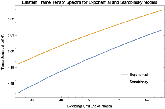
Figure 4: Comparison of the tensor power spectrum Δh2​(k)\Delta^{2}_{h}(k) (left) and the tensor-to-scalar ratio r⁡(k)r(k) (right) for Starobinsky inflation (yellow) and the exponential model (blue). All results are displayed as a function of N~\widetilde{N}, the number of Einstein frame e-foldings before the end of inflation at which horizon crossing occurs.

We studied two models, both of which take the form (1). The first was Starobinsky inflation (54), with the parameter and initial conditions chosen as,

M=10−5,ϵi=0.00221,GH2i=×10−9.M=10^{-5}\qquad,\qquad\epsilon_{i}=0.00221\qquad,\qquad GH^{2}_{i}=7.55\!\times\!10^{-9}\;. (103)

We also studied a model which has been proposed to describe cosmology from inflation to the current phase of acceleration [33],

f⁡(R)=R−Λ⁡[−exp⁡[−(R2​Λ)4]]+R24​Λ.f(R)=R-\Lambda\Biggl[1\!-\!\exp\Bigl[-\Bigl(\frac{R}{2\Lambda}\Bigr)^{4}\Bigr]\Biggr]+\frac{R^{2}}{4\Lambda}\;. (104)

The parameter and initial conditions were chosen as,

GΛ=10−16,ϵi=0.00501,GH2i=×10−15.G\Lambda=10^{-16}\qquad,\qquad\epsilon_{i}=0.00501\qquad,\qquad GH^{2}_{i}=2.22\!\times\!10^{-15}\;. (105)

Despite the different functions f⁡(R)f(R) between (54) and (104), the two models are quite similar as far as inflation is concerned. This shows up clearly from Figure 2 which gives their potentials. Although there are some significant differences for low potential, inflation is governed by the behavior for large potential, which is almost identical.

4.3 Power Spectra of the Two Models

Refer to caption
Refer to caption
Refer to caption
Figure 5: The various spectra — Δℛ2​(k)\Delta^{2}_{\mathcal{R}}(k) (left), Δh2​(k)\Delta^{2}_{h}(k) (middle) and r⁡(k)r(k) (right) — for Starobinsky inflation, as functions of the number of e-foldings from first horizon crossing until the end of inflation. For the yellow plots the xx axes give NN, the number of e-foldings in the Jordan frame, whereas the xx axes of the blue plots give N~\widetilde{N}, the number of e-foldings in the Einstein frame.
Refer to caption
Refer to caption
Refer to caption
Figure 6: The various spectra — Δℛ2​(k)\Delta^{2}_{\mathcal{R}}(k) (left), Δh2​(k)\Delta^{2}_{h}(k) (middle) and r⁡(k)r(k) (right) — for the exponential model, as functions of the number of e-foldings from first horizon crossing until the end of inflation. For the yellow plots the xx axes give NN, the number of e-foldings in the Jordan frame, whereas the xx axes of the blue plots give N~\widetilde{N}, the number of e-foldings in the Einstein frame.

We numerically simulated each model exactly. Figure 3 shows that the scalar power spectrum of the Starobinsky inflation is slightly larger than for exponential model, although both have roughly the same shape. From Figure 4 we see that the tensor power spectrum of Starobinsky inflation slight exceeds that of the exponential model. However, the difference is so slight that the tensor-to-scalar ratio of the exponential model exceeds that of Starobinsky inflation.

Refer to caption
Refer to caption
Refer to caption
Figure 7: Comparison of the exact results (yellow) with the leading slow roll approximation (blue) for Starobinsky inflation. The left graph shows the scalar power spectrum (51), the middle graph shows the tensor power spectrum (52), and the right graph show the tensor-to-scalar ratio (53).
Refer to caption
Refer to caption
Figure 8: Fractional error of our linearized approximation to the scalar (left) and tensor (right) power spectra for Starobinsky inflation.

Figure 5 displays the spectra of the Starobinsky model as functions of the number of e-foldings NN to the end of inflation in the Jordan frame, and the number of e-foldings N~\widetilde{N} to the end of inflation in the Einstein frame. In each case, features at NN appear to be displaced to N~≃N−12​ln⁡(1+2​N)\widetilde{N}\simeq N-\frac{1}{2}\ln(1+2N), in agreement with equation(66). Figure 6 gives the relation between NN and N~\widetilde{N} for the exponential model.

4.4 Comparison with Analytic Results

A major point of this paper has been to develop good analytic approximations for how the power spectra of f⁡(R)f(R) models depend functionally upon the geometry. For all the spectra, and for both models, the leading slow roll approximations are pretty accurate,

Δℛ2​(k)\displaystyle\Delta^{2}_{\mathcal{R}}(k) ≃\displaystyle\simeq G​H~2​(t~k)π​ϵ~​(t~k)≃G​H2​(tk)2​π​ϵ​(tk),\displaystyle\frac{G\widetilde{H}^{2}(\widetilde{t}_{k})}{\pi\widetilde{\epsilon}(\widetilde{t}_{k})}\simeq\frac{GH^{2}(t_{k})}{2\pi\epsilon(t_{k})}\;, (106)
Δh2​(k)\displaystyle\Delta^{2}_{h}(k) ≃\displaystyle\simeq 16π​G​H~2​(t~k)≃24π​G​H2​(tk)​ϵ​(tk),\displaystyle\frac{16}{\pi}G\widetilde{H}^{2}(\widetilde{t}_{k})\simeq\frac{24}{\pi}\,GH^{2}(t_{k})\epsilon(t_{k})\;, (107)
r⁡(k)\displaystyle r(k) ≃\displaystyle\simeq 16​ϵ~​(t~k)≃48​ϵ2​(tk).\displaystyle 16\widetilde{\epsilon}(\widetilde{t}_{k})\simeq 48\epsilon^{2}(t_{k})\;. (108)

Figure 7 shows this for Starobinsky inflation.

Including the slow roll corrections, and just the linearized approximations for 𝒮⁡(k)\mathcal{S}(k) and 𝒞\mathcal{C}, makes the agreement essentially perfect. Figure 8 shows that the relative error of the scalar power spectrum is less than 0.3%0.3\% for Starobinsky inflation. The relative error for the tensor power spectrum is actually at the 0.002%0.002\% accuracy of our numerical simulation.

5 Discussion

We have developed a good functional form for the primordial power spectra of f⁡(R)f(R) inflation, after discussing (in section 2) the relation between Jordan and Einstein frames. When the Einstein frame potential lacks features, the leading slow roll results (106-108) are accurate. This is shown for Starobinsky inflation by Figure 7. (An f⁡(R)f(R) model will agree with Starobinsky inflation if the parameter X⁡(t)X(t) of equation (49) obeys X⁡(t)≃−ϵ⁡(t)X(t)\simeq-\epsilon(t).) When features are present (for which there continues to be observational support [43]), one gets essentially perfect agreement by using just the first two terms of the nonlocal correction factors (95-98) in expressions (83-84) [26].

One cannot distinguish f⁡(R)f(R) models from scalar potential models with just the power spectra. In section 3 we showed how the same data could be used to reconstruct either kind of model. Even for de Sitter-like models this changes if one has information about what the wave number “kk” means in terms of other scales. There is a shift of 2-3 e-foldings between the same feature of the scalar potential reconstruction and the f⁡(R)f(R) reconstruction, with the scalar potential model feature appearing nearer to the end of inflation. One can see this from Figures 5 and 6.

Finally, we mention that an interesting and very topical application of this formalism is perturbations for Higgs inflation [41, 42]. More generally, scalar models with a nonminimal coupling involve similar conformal transformations between Jordan and Einstein frames.

Acknowledgements

We are grateful for conversations and correspondence with J. Garcia-Bellido and M. Sasaki. This work was partially supported by MINECO (Spain) Project FIS2013-44881-P; by the CSIC I-LINK1019 Project; by a travel grant from the University of Florida International Center, College of Liberal Arts and Sciences, Graduate School and Office of the Provost; by NSF grant PHY-1506513; and by the Institute for Fundamental Theory at the University of Florida.

References

  • [1] A. A. Starobinsky, Phys. Lett. B 91, 99 (1980). doi:10.1016/0370-2693(80)90670-X
  • [2] P. A. R. Ade et al. [Planck Collaboration], arXiv:1502.01589 [astro-ph.CO].
  • [3] P. A. R. Ade et al. [Planck Collaboration], arXiv:1502.02114 [astro-ph.CO].
  • [4] A. Kehagias, A. M. Dizgah and A. Riotto, Phys. Rev. D 89, no. 4, 043527 (2014) doi:10.1103/PhysRevD.89.043527 [arXiv:1312.1155 [hep-th]].
  • [5] S. Capozziello, Int. J. Mod. Phys. D 11, 483 (2002) doi:10.1142/S0218271802002025 [gr-qc/0201033].
  • [6] S. M. Carroll, V. Duvvuri, M. Trodden and M. S. Turner, Phys. Rev. D 70, 043528 (2004) doi:10.1103/PhysRevD.70.043528 [astro-ph/0306438].
  • [7] S. Nojiri and S. D. Odintsov, Phys. Rev. D 68, 123512 (2003) doi:10.1103/PhysRevD.68.123512 [hep-th/0307288].
  • [8] S. Capozziello and M. De Laurentis, Phys. Rept. 509, 167 (2011) doi:10.1016/j.physrep.2011.09.003 [arXiv:1108.6266 [gr-qc]].
  • [9] S. Nojiri and S. D. Odintsov, Phys. Rept. 505, 59 (2011) doi:10.1016/j.physrep.2011.04.001 [arXiv:1011.0544 [gr-qc]].
  • [10] N. Makino and M. Sasaki, Prog. Theor. Phys. 86, 103 (1991). doi:10.1143/PTP.86.103
  • [11] N. Deruelle and M. Sasaki, Springer Proc. Phys. 137, 247 (2011) doi:10.1007/978-3-642-19760-4_23 [arXiv:1007.3563 [gr-qc]].
  • [12] M. Li, Phys. Lett. B 736, 488 (2014) Erratum: [Phys. Lett. B 747, 562 (2015)] doi:10.1016/j.physletb.2014.08.008, 10.1016/j.physletb.2015.06.021 [arXiv:1405.0211 [hep-th]].
  • [13] J. O. Gong, J. c. Hwang, W. I. Park, M. Sasaki and Y. S. Song, JCAP 1109, 023 (2011) doi:10.1088/1475-7516/2011/09/023 [arXiv:1107.1840 [gr-qc]].
  • [14] F. Briscese, E. Elizalde, S. Nojiri and S. D. Odintsov, Phys. Lett. B 646, 105 (2007) doi:10.1016/j.physletb.2007.01.013 [hep-th/0612220].
  • [15] S. Bahamonde, S. D. Odintsov, V. K. Oikonomou and M. Wright, arXiv:1603.05113 [gr-qc].
  • [16] A. Y. Kamenshchik, E. O. Pozdeeva, S. Y. Vernov, A. Tronconi and G. Venturi, arXiv:1602.07192 [gr-qc].
  • [17] G. Domènech and M. Sasaki, arXiv:1602.06332 [gr-qc].
  • [18] P. Kuusk, M. Rünkla, M. Saal and O. Vilson, arXiv:1605.07033 [gr-qc].
  • [19] S. Capozziello, S. Nojiri, S. D. Odintsov and A. Troisi, Phys. Lett. B 639, 135 (2006) doi:10.1016/j.physletb.2006.06.034 [astro-ph/0604431].
  • [20] L. Sebastiani, G. Cognola, R. Myrzakulov, S. D. Odintsov and S. Zerbini, Phys. Rev. D 89, no. 2, 023518 (2014) doi:10.1103/PhysRevD.89.023518 [arXiv:1311.0744 [gr-qc]].
  • [21] M. Artymowski, Z. Lalak and M. Lewicki, Phys. Lett. B 750, 595 (2015) doi:10.1016/j.physletb.2015.09.076 [arXiv:1508.05150 [gr-qc]].
  • [22] S. D. Odintsov and V. K. Oikonomou, Class. Quant. Grav. 32, no. 23, 235011 (2015) doi:10.1088/0264-9381/32/23/235011 [arXiv:1504.01772 [gr-qc]].
  • [23] K. Bamba, S. Nojiri, S. D. Odintsov and D. Sáez-Gómez, Phys. Rev. D 90, 124061 (2014) doi:10.1103/PhysRevD.90.124061 [arXiv:1410.3993 [hep-th]].
  • [24] M. G. Romania, N. C. Tsamis and R. P. Woodard, JCAP 1208, 029 (2012) doi:10.1088/1475-7516/2012/08/029 [arXiv:1207.3227 [astro-ph.CO]].
  • [25] D. J. Brooker, N. C. Tsamis and R. P. Woodard, Phys. Rev. D 93, no. 4, 043503 (2016) doi:10.1103/PhysRevD.93.043503 [arXiv:1507.07452 [astro-ph.CO]].
  • [26] D. J. Brooker, N. C. Tsamis and R. P. Woodard, arXiv:1605.02729 [gr-qc].
  • [27] D. J. Brooker, N. C. Tsamis and R. P. Woodard, arXiv:1603.06399 [astro-ph.CO].
  • [28] D. Polarski and A. A. Starobinsky, Phys. Lett. B 356, 196 (1995) doi:10.1016/0370-2693(95)00842-9 [astro-ph/9505125].
  • [29] J. Garcia-Bellido and D. Wands, Phys. Rev. D 52, 6739 (1995) doi:10.1103/PhysRevD.52.6739 [gr-qc/9506050].
  • [30] M. Sasaki and E. D. Stewart, Prog. Theor. Phys. 95, 71 (1996) doi:10.1143/PTP.95.71 [astro-ph/9507001].
  • [31] L. G. Jaime, L. Patino and M. Salgado, Phys. Rev. D 83, 024039 (2011) doi:10.1103/PhysRevD.83.024039 [arXiv:1006.5747 [gr-qc]].
  • [32] D. S. Salopek, J. R. Bond and J. M. Bardeen, Phys. Rev. D 40, 1753 (1989). doi:10.1103/PhysRevD.40.1753
  • [33] E. Elizalde, S. Nojiri, S. D. Odintsov, L. Sebastiani and S. Zerbini, Phys. Rev. D 83, 086006 (2011) doi:10.1103/PhysRevD.83.086006 [arXiv:1012.2280 [hep-th]].
  • [34] N. C. Tsamis and R. P. Woodard, Annals Phys. 267, 145 (1998) doi:10.1006/aphy.1998.5816 [hep-ph/9712331].
  • [35] T. D. Saini, S. Raychaudhury, V. Sahni and A. A. Starobinsky, Phys. Rev. Lett. 85, 1162 (2000) doi:10.1103/PhysRevLett.85.1162 [astro-ph/9910231].
  • [36] S. Nojiri and S. D. Odintsov, Gen. Rel. Grav. 38, 1285 (2006) doi:10.1007/s10714-006-0301-6 [hep-th/0506212].
  • [37] S. Capozziello, S. Nojiri and S. D. Odintsov, Phys. Lett. B 634, 93 (2006) doi:10.1016/j.physletb.2006.01.065 [hep-th/0512118].
  • [38] R. P. Woodard, Lect. Notes Phys. 720, 403 (2007) doi:10.1007/978-3-540-71013-4_14 [astro-ph/0601672].
  • [39] Z. K. Guo, N. Ohta and Y. Z. Zhang, Mod. Phys. Lett. A 22, 883 (2007) doi:10.1142/S0217732307022839 [astro-ph/0603109].
  • [40] A. R. Liddle, P. Parsons and J. D. Barrow, Phys. Rev. D 50, 7222 (1994) doi:10.1103/PhysRevD.50.7222 [astro-ph/9408015].
  • [41] F. L. Bezrukov and M. Shaposhnikov, Phys. Lett. B 659, 703 (2008) doi:10.1016/j.physletb.2007.11.072 [arXiv:0710.3755 [hep-th]].
  • [42] F. Bezrukov, A. Magnin, M. Shaposhnikov and S. Sibiryakov, JHEP 1101, 016 (2011) doi:10.1007/JHEP01(2011)016 [arXiv:1008.5157 [hep-ph]].
  • [43] D. K. Hazra, A. Shafieloo, G. F. Smoot and A. A. Starobinsky, arXiv:1605.02106 [astro-ph.CO].