DESY-16-022
de Sitter vacua and supersymmetry breaking
in six-dimensional flux compactifications
Wilfried Buchmuller11 1 E-mail: wilfried.buchmueller@desy.de, Markus Dierigl22 2 E-mail: markus.dierigl@desy.de, Fabian Ruehle33 3 E-mail: fabian.ruehle@desy.de, Julian Schweizer44 4 E-mail: julian.schweizer@desy.de
Deutsches Elektronen-Synchrotron DESY, 22607 Hamburg, Germany
Abstract
We consider six-dimensional supergravity with Abelian bulk flux compactified on an orbifold. The effective low-energy action can be expressed in terms of chiral moduli superfields with a gauged shift symmetry. The -term potential contains two Fayet-Iliopoulos terms which are induced by the flux and by the Green-Schwarz term canceling the gauge anomalies, respectively. The Green-Schwarz term also leads to a correction of the gauge kinetic function which turns out to be crucial for the existence of Minkowski and de Sitter vacua. Moduli stabilization is achieved by the interplay of the -term and a nonperturbative superpotential. Varying the gauge coupling and the superpotential parameters, the scale of the extra dimensions can range from the GUT scale down to the TeV scale. Supersymmetry is broken by - and -terms, and the scale of gravitino, moduli, and modulini masses is determined by the size of the compact dimensions.
1 Introduction
The ultraviolet completion of the Standard Model remains a challenging question. There are strong theoretical arguments for supersymmetry at high scales and, in connection with gravity and string theory, also for compact extra dimensions. But in the absence of any hint for supersymmetry from the LHC the scale of supersymmetry breaking is completely unknown, except for a lower bound of TeV.
In this connection higher-dimensional theories are of interest which relate the scale of supersymmetry breaking to the size of compact dimensions via quantized magnetic flux [1]. In the context of the heterotic string it has been argued that five or six dimensions are a plausible intermediate step on the way from 10d string theory to a 4d supersymmetric extension of the Standard Model [2, 3, 4, 5], and compactifications to six dimensions (6d) are also very interesting from the perspective of type IIB string theory and F-theory [6, 7, 8]. Furthermore, 6d theories are interesting from a phenomenological point of view. They can naturally explain the multiplicity of quark-lepton generations as a topological quantum number of vacua with magnetic flux [9] and, when compactified on orbifolds, they provide an appealing explanation of the doublet-triplet splitting in unified theories [10, 11, 12, 13]. Orbifold compactifications with flux combine both virtues [14], leading to 4d theories reminiscent of “split” [15, 16] or “spread” [17] supersymmetry.
Many aspects of 6d supergravity theories have already been studied in detail in the past. This includes the complete Lagrangian with matter and gauge fields [18, 19], compactification of gauged supergravity with a monopole background [20], localized Fayet-Iliopoulos terms generated by quantum corrections [21], singular gauge fluxes at the fixed points [22] and the cancellation of bulk and fixed point anomalies by the Green-Schwarz mechanism [23, 24, 25, 26]. In particular, it has been shown in [27] how magnetic flux together with a nonperturbative superpotential can stabilize both dilaton and volume modulus.
The present paper extends our previous work [28] where we showed that the Green-Schwarz mechanism also cancels the anomalies due to the chiral zero modes induced by the magnetic flux. We now demonstrate that the low-energy effective Lagrangian takes the form of an supergravity model for the moduli superfields with a gauged shift symmetry. The corresponding Killing vectors are induced by the magnetic flux and also by the Green-Schwarz term, respectively. Furthermore, supersymmetry implies an important modification of the gauge kinetic function. As discussed already in [29], this allows for a new class of metastable de Sitter solutions.
The paper is organized as follows. In Section 2 we derive the Kähler potential, the gauge kinetic function and the -term potential of the 4d theory with special emphasis on the effects of the Green-Schwarz term. Minkowski and de Sitter vacua are analyzed in Section 3 and it is shown how dilaton, volume and shape moduli can be stabilized by the flux together with a nonperturbative superpotential. The vector boson mass, the charged scalar mass, the moduli masses, and the axion masses are evaluated for two examples of Minkowski vacua with different size of the compact dimensions. An important aspect of the model is the realization of the super-Higgs mechanism with combined - and -term breaking of supersymmetry. This, together with the modulini masses, is discussed in Section 4. Details of the search for de Sitter vacua and the super-Higgs mechanism are given in Appendix A and Appendix B, respectively. Appendix C contains more details about the example models, including numerical values for their mass spectra.
2 Effective supergravity action
Let us first consider the bosonic part of the six-dimensional supergravity action with a gauge field11 1 We use the differential geometry conventions of [30], the volume form multiplying is understood.,
| (1) |
involving the Ricci scalar , the dilaton , the gauge field and the antisymmetric tensor field . The corresponding fields strengths are given by
| (2) |
is the 6d Planck mass and denotes the 6d gauge coupling of mass dimension . The 3-form is the difference between the Chern-Simons forms and for the spin connection and the gauge field , respectively. In the following we ignore since we will not discuss gravitational anomalies, i.e.,
| (3) |
We choose as background geometry the product space with the metric
| (4) |
where correspond to the 4d Minkowski space and to the internal space. It is convenient to use dimensionless coordinates for the compact space, , where is a fixed physical length scale. The rescaling by the dimensionless radion field in (4) leads to standard kinetic terms for the moduli. The shape of the internal space is parametrized by the two real shape moduli in the two-dimensional metric ,
| (5) |
and the orbifold projection acts as . The physical volume of the internal space is , where is the vacuum expectation value of the radion field .
Neglecting the gravitational backreaction on the geometry of the internal space, a constant bulk flux is a solution of the equations of motion,
| (6) |
where . Furthermore, we add to the gauge-gravity sector a bulk hypermultiplet containing a 6d Weyl fermion with charge and two complex scalars. The hypermultiplet can be decomposed into two 4d chiral multiplets with charges and , respectively. The two complex scalars, and , have gauge interactions and a scalar potential which, in 4d language, corresponds to an -term and a -term potential of the two chiral multiplets [31],
| (7) |
Due to charge quantization the value of the background flux can only take discrete values,
| (8) |
For , the index theorem guarantees the presence of massless left-handed 4d Weyl fermions [9]. This model is anomalous, with bulk and fixed point anomalies calculated in [24],
| (9) |
where , , and
| (10) |
where the correspond to the four fixed points on the orbifold. From the first term in Eq. (9) it is obvious that the background flux contributes to the chiral anomaly. As shown in [28], all these anomalies are canceled by the Green-Schwarz term
| (11) |
It is now straightforward to compute the 4d effective action by means of dimensional reduction. Matching the Ricci scalars and the gauge kinetic terms yields for the tree level 4d Planck mass and the 4d gauge coupling, respectively,
| (12) |
The gauge part of the 4d effective action has been worked out in [28]. The field strength of the antisymmetric tensor can be written as
| (13) |
where , and denote 4d scalar, vector and tensor fields. Trading for the dual scalar by means of the Lagrange multiplier term
| (14) |
replacing radion and dilaton by the moduli fields and ,
| (15) |
rescaling the lowest state of the matter field, , and dropping the ‘hat’ for the 4d vector field, one obtains
| (16) |
For convenience, we have introduced the dimensionless parameter
| (17) |
and we have dropped22 2 On the orbifold without flux is projected out. In the case with flux it belongs to the first exited Landau level (). Its tree-level mass is degenerate with the lowest level () of , but for the following discussion is irrelevant. the matter field . Note that the 6d Ricci scalar contains the 4d Ricci scalar and the kinetic terms of the moduli fields , and . For , the scalar corresponding to the 4d zero mode , the flux generates the mass term
| (18) |
For a vacuum expectation value a constant Weyl rescaling has to be performed such that the rescaled metric describes physical 4d distances. The Ricci scalar of the rescaled metric is then multiplied by . corresponds to the physical Planck mass and is related to by the physical volume, . Analogously, the physical coupling is related to by . Furthermore, we now rescale moduli and matter fields, , . The resulting final 4d bosonic action is identical to Eq. (16) except for a change of parameters,
| (19) |
where and are physical Planck mass and gauge coupling, respectively. The parameter is replaced by
| (20) |
and the scalar mass is given by
| (21) |
By construction, the rescaled moduli fields satisfy . We conclude that given a vacuum field configuration one can always perform a rescaling such that the new metric describes physical 4d distances and the new moduli fields satisfy . The length scale corresponds to the physical size of the extra dimensions in terms of the physical Planck mass. In the following we shall therefore directly search for vacua with , and we set .
The flux compactification on the orbifold should lead to a 4d theory with spontaneously broken supersymmetry. Indeed, introducing the complex fields
| (22) |
and comparing expression (16) with the standard supergravity Lagrangian [32], one immediately confirms that the kinetic terms of the moduli and the matter field are reproduced by the Kähler potential33 3 We use the same symbol for a chiral superfield and the related complex scalar; the 4d vectorfield is contained in the real superfield .
| (23) |
with the Killing vectors
| (24) |
where we have used the relation (8) from the flux quantization ; the gauge interaction of the matter field corresponds to the Killing vector
| (25) |
From the coefficient of one reads off the gauge kinetic function
| (26) |
whose real part we denote by . At first glance this appears to be at variance with the coefficient of suggesting . Note, however, that with the Green-Schwarz term we have included only part of the one-loop corrections to the effective action. A complete calculation should preserve supersymmetry. Hence, we expect that there are further contributions such that the correct gauge kinetic function is indeed given by Eq. (26), which remains to be confirmed by an explicit calculation. The one-loop corrected gauge kinetic function depends now on the moduli fields and . Such a -dependence has previously been found in heterotic string compactifications as an effect of quantum corrections [33, 34].
Knowing the Killing vectors and the gauge kinetic function, the -term potential is given by [32]
| (27) |
where and
| (28) | ||||
| (29) |
This is the standard -term potential for a charged complex scalar with a field-dependent Fayet-Iliopoulos (FI) term . The scalar potential in Eq. (19) contains the classical part of the -term potential which is given by . It contributes linearly to the tree-level mass of the charged scalar and quadratically to the energy density. Supersymmetry requires the quantum correction in addition, analogously to the gauge kinetic function. We therefore keep in the -term potential, which again should be verified by direct calculation.
Fayet-Iliopoulos terms which are generated at the orbifold fixed points by quantum corrections have been discussed in [21] in the case of zero bulk flux. These FI terms are , their sum and therefore the effective 4d FI term vanishes (), and they are locally canceled by a dynamically generated flux that modifies the zero-mode wave functions. As we have shown, there is a non-vanishing 4d FI term , which follows from the Green-Schwarz term. Following [21], it would be interesting to analyze systematically the interplay between the classical bulk flux and the local quantum flux at the fixed points, and to study their joint effect on the zero-mode wave functions.
3 Moduli stabilization and boson masses
The explicit form of the supersymmetric effective action enables us to determine the masses of the bosons in the theory. For the gauge boson and the charged scalar field the results were already given in [28]. However, the non-trivial effective gauge coupling additionally includes higher order terms44 4 Furthermore, the normalization of the field strength differs compared to that in [28] in order to match the supergravity conventions. that so far have not been incorporated.
The vector boson mass can be extracted form the bilinear term of the 4d gauge field in Eq. (16) and reads
| (30) |
The lowest charged scalar mass originates from the -term potential and includes corrections due to anomaly cancellation and non-trivial gauge kinetic function. This modifies the classical scalar mass term (18) to
| (31) |
Without flux the negative second term, accounting for the quantum corrections induced by anomaly cancellation, leads to a vacuum expectation value for such that the total -term vanishes. For non-vanishing flux, however, and the first term tends to stabilize the scalar field at zero. Consequently, the charged scalars are stabilized at the origin as long as the first, flux induced, term in Eq. (31) dominates, i.e. for
| (32) |
Moreover, the real part of the gauge kinetic function, determining the effective gauge coupling, has to be positive for the theory to be consistent. Because of the negative prefactor of this leads to a restriction of the physical moduli space parametrized by and (see Eq. (26)),
| (33) |
Hence, for the charged fields are always stabilized at zero for and in the physical region of the moduli space55 5 Note that in Eqs. (30)-(33) only the product appears, since . In the following we set .. Furthermore, in this regime the -term contribution to the scalar potential is positive. However, it is obvious that the runaway-type -term potential alone can not stabilize the moduli fields and we have to include a superpotential.
A superpotential for the moduli can arise at the orbifold fixed points in the six-dimensional supergravity theory. The superpotential in the 4d effective action is the sum of the fixed point contributions. Consistency requires this superpotential to be gauge invariant66 6 Unless one gauges an R-symmetry leading to constant FI-terms [35, 36].. In the following discussion we neglect a possible coupling of moduli to charged bulk fields and restrict our attention to a superpotential that only depends on the moduli fields. For that reason we define a gauge invariant combination of the two shifting chiral superfields and
| (34) |
The superpotential is a holomorphic function of and the gauge invariant modulus . Inspired by typical superpotentials induced by nonperturbative effects, such as gaugino condensation or instanton corrections, we assume the following functional dependence
| (35) |
where, without loss of generality, we choose the parameters , , and to be real. For an exponential suppression of these nonperturbative effects we further demand that and are real and positive. The -term scalar potential reads
| (36) |
Note that the Kähler potential (23) is of the no-scale form, and the contribution is therefore canceled. The F-term potential (36) also contributes to the scalar mass term . However, this contribution is , which is much smaller than the leading contribution , and it can therefore be neglected.
With the charged fields stabilized at zero the -term
| (37) |
and the linearly independent combination
| (38) |
can be used to rewrite the scalar potential in the convenient form
| (39) |
where the parameters of the superpotential are encoded in
| (40) |
For the specific form (35) of the superpotential these quantities are given in App. A. In order to find minima with vanishing or small cosmological constant one has to solve the four equations
| (41) |
These are worked out in App. A. We use an inverted procedure to obtain the superpotential parameters by solving Eqs. (41) after fixing the vacuum expectation values of the moduli fields and the energy density. Consequently, for vanishing or small cosmological constant the derived superpotential is fine-tuned to compensate the large positive -term depending on and . To solve Eqs. (41) we further have to fix one of the parameters, which we choose to be . However, one of the above combinations, , can be uniquely determined in terms of the moduli values at the minimum. Up to the prefactor the form is identical to the two moduli case discussed in [29],
| (42) |
where is the ratio . Therefore, the arguments for the existence of vacua given in [29] carry over to the three moduli case. Importantly, one necessary condition is that the prefactor of one of the moduli in the gauge kinetic function is negative. In the above case this constrains the allowed moduli region to a regime where the -terms are positive definite. The additional negative contributions from the -terms of the gauge invariant superpotential allow to find Minkowski or de Sitter vacua with all moduli stabilized. In this way we can construct models with Minkowski or de Sitter vacua with a size of the internal space that ranges between GUT and TeV scale.
Given a vacuum with and the cancellation between - and -term contributions to the potential, we can derive the -dependence of the various parameters and masses. For parametrized by solutions to Eqs. (41) can be found for certain values of the parameter . Keeping this parameter combination fixed we then obtain models with different size of the extra dimensions. Accordingly, the scaling of the effective gauge coupling and -term potential is
| (43) |
This directly implies a scaling of the superpotential parameters
| (44) |
and allows to deduce the behavior of the bosonic masses
| (45) |
Superpotential and boson masses: two examples
In order to illustrate our general results and to get some intuition for the parameters and mass scales involved, we work out explicitly two models exhibiting Minkowski vacua with different size of the internal dimensions. As explained above we start with the choice of the gauge coupling , the size of the compact dimensions, and in the superpotential. The parameters of the two models read
| (46) |
The number of flux quanta in both vacua is set to , which ensures the stabilization of the charged scalar fields, see Eq. (32), and already hints at a multiplicity which can be used in grand unified model building [14]. The complex shape modulus is stabilized at , which corresponds to the square torus assumed in [29].
To achieve in the vacuum we parametrize by as above. Therefore, the mass scale of the internal dimensions (in 4d Planck units) is given by
| (47) |
which corresponds to the GUT scale and an intermediate mass scale, respectively. The moduli are stabilized at , . As discussed above, the combination remains constant in both models. The minima in the two different models are plotted in the - and the - plane in Figures 1 and 2.
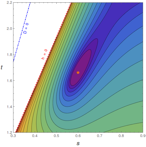

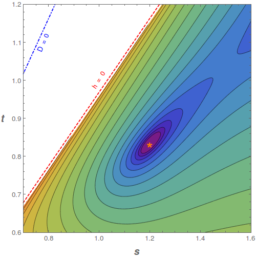

One immediate consistency check for the solutions is the value of the effective gauge coupling which has to be positive and small enough to allow a perturbative treatment
| (48) |
This perfectly matches the scaling behavior in Eq. (43). The charged scalar and vector boson masses can then be evaluated numerically using Eqs. (30) and (31)
| (49) | ||||
Again, the scaling with of Eq. (45) is realized. For the masses of the moduli fields and the axions we need to evaluate the superpotential parameters. From Eq. (44) we would expect a factor of and indeed the respective orders of magnitude are
| (50) |
The numerical values are given in App. C. The nonperturbative exponent in both vacua is . Knowing the superpotential, and after canonical normalization, the eigenvalues of the moduli masses matrix can be calculated,
| (51) |
The eigenvalues are all of the order of the vector boson mass and slightly larger than the gravitino mass. The scaling between the two models matches the one predicted in Eq. (45). The same is true for the two non-vanishing eigenvalues of the axion mass matrix
| (52) |
so that
| (53) |
One massless axion gives mass to the vector boson via the Stückelberg mechanism. Their numerical values in both vacua are discussed in App. C, where the scaling is explicitly demonstrated.
It is instructive to compare the mass spectra of the two models. From Eq. (31) one reads off that in both cases . Hence, even the lightest charged scalar does not belong to the low-energy effective Lagrangian for fields with masses . Nevertheless, we included this scalar in the above discussion to check the stability of the vacuum, that is . The vector boson, moduli and axion masses scale as and become parametrically smaller than the size of the extra dimension for large .
4 Super-Higgs mechanism and fermion masses
The first step in calculating the fermion masses is to disentangle their mixing with the gravitino, i.e. to identify the Goldstino. Since supersymmetry is broken by - and -terms, the Goldstino is a mixture of the gaugino and modulini. Charged fermions do not contribute as long as their scalar partners have vanishing vacuum expectation values. We can therefore restrict our discussion to the gaugino and modulini, and we also assume a ground state with vanishing cosmological constant.
The bilinear fermionic Lagrangian involves kinetic, mass, and mixing terms for the gravitino, gaugino and modulini fields. All these terms are determined by the Kähler potential, the superpotential, the Killing vectors and the gauge kinetic function of the model. The terms involving the gravitino are [32]
| (54) |
where is a linear combination of the fermions in the theory, and the gravitino mass is given by77 7 In the following, bosonic terms are understood as expectation values in the ground state.
| (55) |
In the model under consideration this yields
| (56) |
The -term affects the value of the gravitino mass via the expectation values of the moduli fields determined in a vacuum with vanishing cosmological constant.
The fermion in Eq. (54) is the Goldstino. It is given by a linear combination of the gaugino and modulini , determined by - and -terms,
| (57) |
It is well known that the mixing terms in Eq. (54) can be removed via a local field redefinition of the gravitino [32],
| (58) |
With this shift, a straightforward calculation yields for the Lagrangian, (54)
| (59) |
Note that the kinetic term of has the sign of a ghost. The kinetic term and the mass term of lead to modifications of the kinetic terms and the mass matrix of gaugino and modulini whereas the mass term for the gravitino remains unchanged.
Eq. (59) represents the gravitino Lagrangian in unitary gauge. Hence, the dependence on the Goldstino should completely disappear in the full Lagrangian, which we explicitly demonstrate in the following. The kinetic terms of gaugino and modulini read
| (60) |
Since the Kähler metric is hermitian, it can be diagonalized by a unitary transformation. Moreover, the real eigenvalues are all positive for the kinetic terms to be well-defined. Hence, one can rescale the eigenvalues to one by conjugation with a real diagonal matrix. The combined transformation corresponds to a vielbein for the Kähler metric,
| (61) |
It is convenient to redefine gaugino and modulini,
| (62) |
such that their kinetic terms are canonical,
| (63) |
the new index labels gaugino () and modulini (). One can now perform a unitary transformation which rotates the canonically normalized fermions into and three orthogonal Weyl fermions
| (64) |
From Eqs. (57) and (58) one obtains for the matrix elements of the inverse transformation,
| (65) |
One easily verifies the unitarity condition for the -component,
| (66) |
where we used . Clearly, in Minkowski space one has . Since all fermions are canonically normalized the kinetic terms for the orthogonal Weyl fermions and are given by
| (67) |
Combined with Eq. (59) the kinetic terms for cancel, as expected in the unitary gauge.
Furthermore, we expect the mass eigenvalue of the Goldstino and its mixing terms with the other fermions to vanish. In order to show this, we express the fermion bilinears in terms of the canonically normalized gaugino and modulini,
| (68) |
The mass matrix elements are given in App. B. Inserting (64), one obtains for the mass term and mixing of the Goldstino field the expressions
| (69) |
Using the explicit form of the fermion mass matrix and Eqs. (65), a straightforward calculation yields (see App. B)
| (70) |
which indeed vanishes in Minkowski space for a gauge invariant superpotential. Analogously, one finds
| (71) |
which also vanishes in Minkowski space for an extremum of the scalar potential. Hence, the Goldstino indeed decouples from the mass matrix.
In summary, we obtain from Eqs. (59), (67) and (69),
| (72) |
where
| (73) |
is the mass matrix of the fermions orthogonal to the Goldstino. Again, the cancellation of - and -terms for small cosmological constant allows to derive a general scaling behavior for the fermion masses. With Eqs. (43) and (44) we obtain
| (74) |
Gravitino and fermion masses: two examples
Using the expression (56) for the gravitino mass one obtains for the two models defined by Eqs. (46) and the vacuum values of the moduli fields ,
| (75) |
The modulini masses are evaluated numerically from Eq. (87). As expected, one finds one eigenvector with zero mass, the Goldstino. The three remaining fermion fields are massive with mass eigenvalues of order the gravitino mass
| (76) |
Again, the explicit numerical values and scaling behaviors are summarized in App. C. An overview over the mass spectrum in both vacua is provided in Fig. 3. Interestingly, in both of the vacua one modulini field remains lighter than the gravitino whereas the other two are slightly heavier.
5 Summary and Outlook
We have analyzed a 6d supergravity model compactified to 4d on an orbifold. Using bulk flux, a nonperturbative superpotential, and the Green-Schwarz term for anomaly cancellation we obtained 4d de Sitter or Minkowski vacua where all moduli are stabilized. This allows for an explicit computation of the masses of all particles in the effective low-energy theory.
In the model under discussion, supersymmetry is broken by both - and -terms. By analyzing the bosonic 6d effective action, we extracted the -term potential resulting from the FI parameter of the anomalous , which receives contributions from the Green-Schwarz term and from the bulk flux. From the Green-Schwarz term we also obtained an important correction to the gauge kinetic function. The -term potential results from our choice of the superpotential which is of the KKLT-type. Knowing the complete scalar potential we then calculated the boson masses which depend on the superpotential parameters and the flux.
For the discussion of the fermion masses we have studied the super-Higgs mechanism in the presence of - and -term breaking. Via a rotation in field space we extracted the Goldstino which is eaten by the gravitino in unitary gauge. The Goldstino indeed completely drops out of the Lagrangian, as we explicitly verified using the extremum conditions of the scalar potential for Minkowski space and the gauge invariance of the superpotential.
In order to find vacua of our effective theory that are de Sitter or Minkowski and are within a reasonable parameter range for the moduli, we inverted the problem: Choosing a gauge coupling and the size of the extra dimensions, and starting from a point in moduli space we derived equations for the superpotential parameters for which the scalar potential is minimized. Having obtained the parameters of our effective theory that way, we inserted the parameters back into the scalar potential which we then minimized. As a cross-check, we found the minimum exactly at the point in moduli space which we used to obtain the parameters in the inverted problem.
Finally, we discussed two example models with different parameters and evaluated numerically the masses of all particles in the model. In the first example, the extra dimensions are of order the GUT scale, , and moduli, axion and gauge boson masses are also , slightly larger than gravitino and modulini masses. In the second example, the size of the extra dimensions corresponds to an intermediate scale, and all masses scale as . The only exception is the charged scalar mass which is of the order of the compactification scale. The size of the extra dimensions is controlled by the gauge coupling, with . This dependence on the gauge coupling can be used to construct models whose size of the extra dimensions interpolates between the GUT scale and the TeV scale.
The constructed family of de Sitter vacua can easily be combined with higher-dimensional GUT models, and they also offer an interesting playground to study the interplay of moduli stabilization and inflation. Since the considered 6d flux compactifications contain all ingredients familiar from string models, i.e. compact dimensions with flux, the Green-Schwarz mechanism and a nonperturbative superpotential, it will be very interesting to see whether they can in fact be realized within a string theory construction.
Acknowledgments
We thank Emilian Dudas, Zygmunt Lalak, Jan Louis, Hans-Peter Nilles, and Alexander Westphal for valuable discussions. This work was supported by the German Science Foundation (DFG) within the Collaborative Research Center (SFB) 676 “Particles, Strings and the Early Universe”. M.D. also acknowledges support from the Studienstiftung des deutschen Volkes.
Appendix A Parameters for de Sitter and Minkowski vacua
For the evaluation of the superpotential parameters it is convenient to define new linear combinations of the derivative operators
| (77) |
In terms of this derivative operators the constraints (41) can be rewritten as (note that )
| (78) |
Using the specific form of the nonperturbative superpotential (35) the parameters can be identified as:
| (79a) | ||||
| (79b) | ||||
| (79c) | ||||
| (79d) | ||||
Under the assumption and the imaginary parts are generically stabilized at zero. Nevertheless, this has to be checked a posteriori for the specific superpotential parameters. In the following we will therefore set and and crosscheck for consistency afterward. We further introduce a convenient new combination
| (80) |
Using the relations
| (81) |
and analogous equations for , where is substituted by , as well as
| (82) |
one finds
| (83a) | ||||
| (83b) | ||||
| (83c) | ||||
Here, we have introduced the linear combination .
One can then reverse the problem of finding a minimum of the scalar potential for fixed parameters by fixing the values of the moduli and trying to solve Eqs. (77) for the superpotential parameters instead. It is obvious that the superpotential (35) has five free parameters, but we only have four equations to determine them. Therefore, generically we have to fix one of the parameters in order to solve for the others88 8 It is a natural choice to fix which corresponds to nonperturbative effects in ..
The solution for the superpotential parameters has to fulfill several consistency conditions. For instance, taking into account Eqs. (79a) and (79b), and have to be positive. Interestingly, the combination of the equations with the constraint that , fixes unambiguously
| (84) |
where we have introduced the new variable . Unfortunately, the rest of the equations can not be simplified in a similar way and have to be evaluated numerically.
Appendix B Fermion masses
In the following we derive the mass matrix for canonically normalized fermions and show explicitly that the Goldstino decouples in the unitary gauge.
The standard fermion mass terms for gaugino and modulini are given in full generality in [32]. For our case they read
| (85) |
where (with etc.). After the rescaling to canonical kinetic terms (62) and transforming to the unitary gauge (58), the fermion bilinears are given by
| (86) |
Using [32], the mass matrix elements read
| (87) |
In order to show the decoupling of the Goldstino we now perform the unitary transformation to the basis, for which we have to show . Using the above expressions for and Eq. (65) for one obtains
| (88) |
where we used . Clearly, the gauge invariance of the superpotential, i.e , implies that in Minkowski space
| (89) |
Similarly, one finds for the second condition
| (90) |
where we have used the identity
| (91) |
From Eq. (90) one reads off that
| (92) |
for an extremum of the potential and vanishing vacuum energy density.
As expected, for a gauge invariant superpotential the Goldstino completely decouples from the mass matrix at an extremum of the potential with vanishing cosmological constant. In the case of a small cosmological constant the above equations are modified by terms .
Appendix C Numerical evaluation of masses
We summarize the superpotential parameters and masses of the bosons and fermions in the two vacua (46) with different sizes of the extra dimensions and demonstrate the predicted scaling behavior. The vacuum expectation values for the moduli in the vacuum are
| (93) |
The other input parameters for the two models are
| (94) |
corresponding to a scale parameter of . In order to obtain unique solutions for the superpotential we have to fix one of its parameters, see App. A. Therefore, we choose and . The numerical values for the superpotential parameters and their scaling behavior are summarized in Tab. 1.
With the parameters of the superpotential the moduli, axion, and modulini masses can also be calculated numerically (after canonical normalization of the kinetic term). The mass eigenvalues are summarized in Tab. 2. The scaling with respect to the size of the extra dimensions matches nicely the expressions in (45) and (74). Both mass hierarchies are depicted in a logarithmic scale in Fig. 3.
References
- [1] C. Bachas “A Way to break supersymmetry,” [hep-th/9503030].
- [2] T. Kobayashi, S. Raby, and R.-J. Zhang “Constructing 5-D orbifold grand unified theories from heterotic strings,” Phys. Lett. B593 (2004) 262–270 [hep-ph/0403065].
- [3] S. Forste, H. P. Nilles, P. K. S. Vaudrevange, and A. Wingerter “Heterotic brane world,” Phys. Rev. D70 (2004) 106008 [hep-th/0406208].
- [4] A. Hebecker and M. Trapletti “Gauge unification in highly anisotropic string compactifications,” Nucl. Phys. B713 (2005) 173–203 [hep-th/0411131].
- [5] W. Buchmuller, C. Ludeling, and J. Schmidt “Local SU(5) Unification from the Heterotic String,” JHEP 09 (2007) 113 [0707.1651].
- [6] R. Blumenhagen, V. Braun, B. Kors, and D. Lust “Orientifolds of K3 and Calabi-Yau manifolds with intersecting D-branes,” JHEP 07 (2002) 026 [hep-th/0206038].
- [7] W. Taylor “TASI Lectures on Supergravity and String Vacua in Various Dimensions,” [1104.2051].
- [8] C. Lüdeling and F. Ruehle “F-theory duals of singular heterotic K3 models,” Phys. Rev. D91 (2015) no. 2, 026010 [1405.2928].
- [9] E. Witten “Some Properties of O(32) Superstrings,” Phys. Lett. B149 (1984) 351–356.
- [10] Y. Kawamura “Triplet doublet splitting, proton stability and extra dimension,” Prog. Theor. Phys. 105 (2001) 999–1006 [hep-ph/0012125].
- [11] L. J. Hall and Y. Nomura “Gauge unification in higher dimensions,” Phys. Rev. D64 (2001) 055003 [hep-ph/0103125].
- [12] A. Hebecker and J. March-Russell “A Minimal S**1 / (Z(2) x Z-prime (2)) orbifold GUT,” Nucl. Phys. B613 (2001) 3–16 [hep-ph/0106166].
- [13] T. Asaka, W. Buchmuller, and L. Covi “Gauge unification in six-dimensions,” Phys. Lett. B523 (2001) 199–204 [hep-ph/0108021].
- [14] W. Buchmuller, M. Dierigl, F. Ruehle, and J. Schweizer “Split symmetries,” Phys. Lett. B750 (2015) 615–619 [1507.06819].
- [15] N. Arkani-Hamed and S. Dimopoulos “Supersymmetric unification without low energy supersymmetry and signatures for fine-tuning at the LHC,” JHEP 06 (2005) 073 [hep-th/0405159].
- [16] G. F. Giudice and A. Romanino “Split supersymmetry,” Nucl. Phys. B699 (2004) 65–89 [hep-ph/0406088]. [Erratum: Nucl. Phys.B706,487(2005)].
- [17] L. J. Hall and Y. Nomura “Spread Supersymmetry,” JHEP 01 (2012) 082 [1111.4519].
- [18] H. Nishino and E. Sezgin “Matter and Gauge Couplings of N=2 Supergravity in Six-Dimensions,” Phys. Lett. B144 (1984) 187–192.
- [19] H. Nishino and E. Sezgin “The Complete , Supergravity With Matter and Yang-Mills Couplings,” Nucl. Phys. B278 (1986) 353–379.
- [20] Y. Aghababaie, C. P. Burgess, S. L. Parameswaran, and F. Quevedo “SUSY breaking and moduli stabilization from fluxes in gauged 6-D supergravity,” JHEP 03 (2003) 032 [hep-th/0212091].
- [21] H. M. Lee, H. P. Nilles, and M. Zucker “Spontaneous localization of bulk fields: The Six-dimensional case,” Nucl. Phys. B680 (2004) 177–198 [hep-th/0309195].
- [22] G. von Gersdorff “Anomalies on Six Dimensional Orbifolds,” JHEP 03 (2007) 083 [hep-th/0612212].
- [23] J. Erler “Anomaly cancellation in six-dimensions,” J. Math. Phys. 35 (1994) 1819–1833 [hep-th/9304104].
- [24] T. Asaka, W. Buchmuller, and L. Covi “Bulk and brane anomalies in six-dimensions,” Nucl. Phys. B648 (2003) 231–253 [hep-ph/0209144].
- [25] C. A. Scrucca and M. Serone “Anomalies in field theories with extra dimensions,” Int. J. Mod. Phys. A19 (2004) 2579–2642 [hep-th/0403163].
- [26] D. S. Park and W. Taylor “Constraints on 6D Supergravity Theories with Abelian Gauge Symmetry,” JHEP 01 (2012) 141 [1110.5916].
- [27] A. P. Braun, A. Hebecker, and M. Trapletti “Flux Stabilization in 6 Dimensions: D-terms and Loop Corrections,” JHEP 02 (2007) 015 [hep-th/0611102].
- [28] W. Buchmuller, M. Dierigl, F. Ruehle, and J. Schweizer “Chiral fermions and anomaly cancellation on orbifolds with Wilson lines and flux,” Phys. Rev. D92 (2015) no. 10, 105031 [1506.05771].
- [29] W. Buchmuller, M. Dierigl, F. Ruehle and J. Schweizer, Phys. Rev. Lett. 116, no. 22, 221303 (2016) [arXiv:1603.00654 [hep-th]].
- [30] R. Blumenhagen, D. Lüst, and S. Theisen Basic Concepts of String Theory. Theoretical and Mathematical Physics. Springer-Verlag Berlin Heidelberg 2012.
- [31] N. Arkani-Hamed, T. Gregoire, and J. G. Wacker “Higher dimensional supersymmetry in 4-D superspace,” JHEP 03 (2002) 055 [hep-th/0101233].
- [32] J. Wess and J. Bagger Supersymmetry and supergravity. 1992.
- [33] L. E. Ibanez and H. P. Nilles “Low-Energy Remnants of Superstring Anomaly Cancellation Terms,” Phys. Lett. B169 (1986) 354–358.
- [34] L. J. Dixon, V. Kaplunovsky, and J. Louis “Moduli dependence of string loop corrections to gauge coupling constants,” Nucl. Phys. B355 (1991) 649–688.
- [35] G. Villadoro and F. Zwirner “De-Sitter vacua via consistent D-terms,” Phys. Rev. Lett. 95 (2005) 231602 [hep-th/0508167].
- [36] I. Antoniadis and R. Knoops “Gauge R-symmetry and de Sitter vacua in supergravity and string theory,” Nucl. Phys. B886 (2014) 43–62 [1403.1534].