Supercloseness of the SDFEM on Shishkin triangular meshes for problems with exponential layers

Jin Zhang Corresponding author: Corresponding author: jinzhangalex@hotmail.com Address: School of Mathematical Sciences, Shandong Normal University, Jinan 250014, China Xiaowei Liu Note: Email: xwliuvivi@hotmail.com Address: College of Science, Qilu University of Technology, Jinan 250353, China.

Abstract

In this paper, we analyze the supercloseness property of the streamline diffusion finite element method (SDFEM) on Shishkin triangular meshes, which is different from one in the case of rectangular meshes. The analysis depends on integral inequalities for the part related to the diffusion in the bilinear form. Moreover, our result allows the construction of a simple postprocessing that yields a more accurate solution. Finally, numerical experiments support these theoretical results.

1 Introduction

We consider the singularly perturbed boundary value problem

\begin{array}[]{rcl}-\varepsilon\Delta u+\boldsymbol{b}\cdot\nabla u+cu=f&\mbox{in}&\Omega=(0,1)^{2},\\ u=0&\mbox{on}&\partial\Omega,\end{array}

(1.1)

where $\varepsilon\ll|\boldsymbol{b}|$ is a small positive parameter, the functions $\boldsymbol{b}(x,y)=(b_{1}(x,y),b_{2}(x,y))^{T}$ , $c(x,y)\geq 0$ and $f(x,y)$ are supposed sufficiently smooth. We also assume

b_{1}(x,y)\geq\beta_{1}>0,\,b_{2}(x,y)\geq\beta_{2}>0,\,c(x,y)-\frac{1}{2}\nabla\cdot\boldsymbol{b}(x,y)\geq\mu_{0}>0\quad\text{on $\bar{\Omega},$}

where $\beta_{1}$ , $\beta_{2}$ and $\mu_{0}$ are some constants. The solution of (1.1) typically has two exponential layers of width $O(\varepsilon\ln(1/\varepsilon))$ at the sides $x=1$ and $y=1$ of $\Omega$ .

Because of the presence of layers, standard numerical methods such as the finite element method and the finite difference method, suffer from severe nonphysciall oscillations. Thus, stabilized methods and/or a priori adapted meshes (see [16, 12]) are widely used. In this paper, we are to analyze the streamline diffusion finite element method (SDFEM) [8] on the Shishkin mesh [15]. This combination possesses good numerical stability and high accuracy for problems (1.1), see [11] for detailed numerical tests.

The SDFEM on Shishkin rectangular meshes are widely studied, see [18, 6, 5, 19, 20] and references therein. In these papers, supercloseness results are analyzed for optimal $L^{2}$ estimates, $L^{\infty}$ bounds and postprocessing procedures etc. Here “supercloseness” means convergence order of $u^{I}-u^{N}$ in some norm is greater than one of $u-u^{I}$ , where $u^{I}$ is the interpolant of the solution $u$ from the finite element space, $u^{N}$ is the SDFEM solution. However, to our knowledge, there are no supercloseness results of the SDFEM on triangular meshes, which are one kind of popular grids for two-dimensional domains. The main reason is that there are no analysis tools on triangular meshes similar to Lin’s integral identities [9] which are used to obtain the supercloseness properties in the case of rectangles.

In this work, we present integral inequalities , i.e. Lemma 2.1, for the diffusion part in the bilinear form, by means of which the bound $\|u^{I}-u^{N}\|_{SD}\leq C(\varepsilon^{1/2}N^{-1}+N^{-3/2})\ln^{3/2}N$ is obtained. Based on this result, a simple postprocessing technique is applied to the SDFEM’s solution $u^{N}$ and this procedure yields a more accurate numerical solution. Finally, numerical experiments support our theoretical results.

Here is the outline of this article. In §2 we give some a priori informations of the solution of (1.1), then introduce Shishkin meshes and a streamline diffusion finite element method on these meshes. In §3 we obtain the supercloseness result. In §4 we present the uniform estimate for the postprocessing solution. Finally, some numerical results are presented in §5.

Throughout the article, the standard notations for the Sobolev spaces and norms will be used; and generic constants $C$ , $C_{i}$ are independent of $\varepsilon$ and $N$ . An index will be attached to indicate an inner product or a norm on a subdomain $D$ , for example, $(\cdot,\cdot)_{D}$ and $\|\cdot\|_{D}$ .

2 The SDFEM on Shishkin meshes

In this section we will introduce the apriori informations of the solution, the Shishkin mesh and the SDFEM.

2.1 The regularity results

As mentioned before the solution $u$ of (1.1) possesses two exponential layers at $x=1$ and $y=1$ . For our later analysis we shall suppose that $u$ can be split into a regular solution component and various layer parts:

Assumption 2.1.

Assume that the solution of (1.1) can be decomposed as

u=S+E_{1}+E_{2}+E_{12},\quad\forall(x,y)\in\bar{\Omega}.

(2.1)

For $0\leq i+j\leq 2$ , the regular part satisfies

\left|\frac{\partial^{i+j}S}{\partial x^{i}\partial y^{j}}(x,y)\right|\leq C,

while for $0\leq i+j\leq 3$ , the layer terms satisfy:

\left|\frac{\partial^{i+j}E_{1}}{\partial x^{i}\partial y^{j}}(x,y)\right|\leq C\varepsilon^{-i}e^{-\beta_{1}(1-x)/\varepsilon},

\left|\frac{\partial^{i+j}E_{2}}{\partial x^{i}\partial y^{j}}(x,y)\right|\leq C\varepsilon^{-j}e^{-\beta_{2}(1-y)/\varepsilon},

and

\quad\quad\quad\left|\frac{\partial^{i+j}E_{12}}{\partial x^{i}\partial y^{j}}(x,y)\right|\leq C\varepsilon^{-(i+j)}e^{-(\beta_{1}(1-x)+\beta_{2}(1-y))/\varepsilon}.

Remark 2.1.

Conditions on the data of the problem that guarantee the existence of this decomposition are given in [10, Theorem 5.1].

2.2 Shishkin meshes

When discretizing (1.1), first we divide the domain $\Omega$ into four subdomains (see Figure 2)

		$\displaystyle\Omega_{s}:=\left[0,1-\lambda_{x}\right]\times\left[0,1-\lambda_{y}\right],$		$\displaystyle\Omega_{x}:=\left[1-\lambda_{x},1\right]\times\left[0,1-\lambda_{y}\right],$
		$\displaystyle\Omega_{y}:=\left[0,1-\lambda_{x}\right]\times\left[1-\lambda_{y},1\right],$		$\displaystyle\Omega_{xy}:=\left[1-\lambda_{x},1\right]\times\left[1-\lambda_{y},1\right].$

Here $\lambda_{x}$ and $\lambda_{y}$ are mesh transition parameters which are used to separate the domain $\Omega$ into the smooth part and different layer parts. They are defined as follows:

\lambda_{x}:=\min\left\{\frac{1}{2},\rho\frac{\varepsilon}{\beta_{1}}\ln N\right\}\quad\mbox{and}\quad\lambda_{y}:=\min\left\{\frac{1}{2},\rho\frac{\varepsilon}{\beta_{2}}\ln N\right\}.

In this paper, we set $\rho=2.5$ for technical reasons, see [21, Remark 2.1] for the discussions of the different choices of $\rho$ .

Assumption 2.2.

Assume that $\varepsilon\leq N^{-1}$ , as is generally the case in practice. Furthermore assume that $\lambda_{x}=\rho\varepsilon\beta^{-1}_{1}\ln N$ and $\lambda_{y}=\rho\varepsilon\beta^{-1}_{2}\ln N$ as otherwise $N^{-1}$ is exponentially small compared with $\varepsilon$ .

Each subdomain is then decomposed into $N/2\times N/2$ ( $N\geq 4$ is a positive even integer) uniform rectangles and uniform triangles by drawing the diagonal in each rectangles (see Figure 2). This yields a piecewise uniform triangulation of $\Omega$ denoted by $\mathcal{T}_{N}$ . Therefore, there are $N^{2}$ nodes $(x_{i},y_{j})$ , $i,j=0,1,\ldots,N$ and $2N^{2}$ triangle elements.

We denote $h_{x,i}:=x_{i+1}-x_{i}$ and $h_{y,i}:=y_{i+1}-y_{i}$ which satisfy

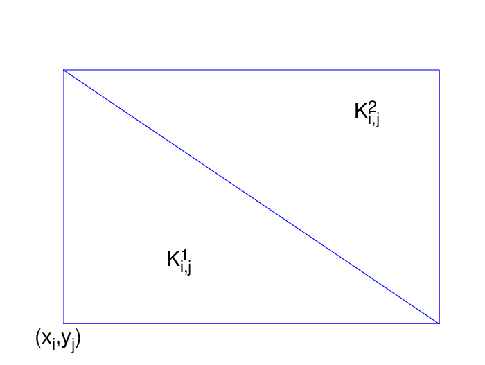
		$\displaystyle N^{-1}\leq h_{x,i},h_{y,i}\leq 2N^{-1}\quad\text{if $i=0,1,\ldots,N/2-1$}$
		$\displaystyle C_{1}\varepsilon N^{-1}\ln N\leq h_{x,i},h_{y,i}\leq C_{2}\varepsilon N^{-1}\ln N.\quad\text{if $i=N/2,N/2+1,\ldots,N-1$}$

For mesh elements we shall use some notations: $K^{1}_{i,j}$ for the mesh triangle with vertices $(x_{i},y_{j})$ , $(x_{i+1},y_{j})$ and $(x_{i},y_{j+1})$ ; $K^{2}_{i,j}$ for the mesh triangle with vertices $(x_{i},y_{j+1})$ , $(x_{i+1},y_{j})$ and $(x_{i+1},y_{j+1})$ (see Fig. 2); $K$ for a generic mesh triangle.

Refer to caption — Fig.1: Dissection of $\Omega$ and triangulation $\mathcal{T}_{N}$ .

2.3 The streamline diffusion finite element method

Let $V:=H^{1}_{0}(\Omega)$ . A weak formulation of the model problem (1.1) reads: Find $u\in V$ such that

\varepsilon(\nabla u,\nabla v)+(\boldsymbol{b}\cdot\nabla u+cu,v)=(f,v),\quad\forall v\in V.

(2.2)

Note that the variational formulation (2.2) has a unique solution by means of the Lax-Milgram Lemma.

Let $V^{N}\subset V$ be the $C^{0}$ linear finite element space on the Shishkin mesh. The SDFEM reads: Find $u^{N}\in V^{N}$ such that

a_{SD}(u^{N},v^{N})=(f,v^{N})+\underset{K\subset\Omega}{\sum}(f,\delta_{K}\boldsymbol{b}\cdot\nabla v^{N})_{K},\quad\forall v^{N}\in V^{N}

(2.3)

where

a_{SD}(u^{N},v^{N})=a_{Gal}(u^{N},v^{N})+a_{stab}(u^{N},v^{N})

and

	$\displaystyle a_{Gal}(u^{N},v^{N})$	$\displaystyle=\varepsilon(\nabla u^{N},\nabla v^{N})+(\boldsymbol{b}\cdot\nabla u^{N}+cu^{N},v^{N})$
	$\displaystyle a_{stab}(u^{N},v^{N})$	$\displaystyle=\sum_{K\subset\Omega}(-\varepsilon\Delta u^{N}+\boldsymbol{b}\cdot\nabla u^{N}+cu^{N},\delta_{K}\boldsymbol{b}\cdot\nabla v^{N})_{K}.$

Note that $\Delta u^{N}=0$ in $K$ for $u^{N}|_{K}\in P_{1}(K)$ . Following usual practice [12], the parameter $\delta_{K}=\delta_{K}(x,y)$ is defined as follows

\delta_{K}:=\left\{\begin{array}[]{cc}C^{\ast}N^{-1},&\text{if $K\subset\Omega_{s}$},\\ 0,&\text{otherwise},\end{array}\right.

(2.4)

where $C^{\ast}$ is a properly defined positive constant such that the following coercivity holds (see [12, Lemma 3.25])

a_{SD}(v^{N},v^{N})\geq\frac{1}{2}\|v^{N}\|^{2}_{SD},\quad\forall v^{N}\in V^{N}.

(2.5)

We define an energy norm associated with $a_{Gal}(\cdot,\cdot)$ and the streamline diffusion norm (SD norm) associated with $a_{SD}(\cdot,\cdot)$ :

	$\displaystyle\\|v^{N}\\|^{2}_{\varepsilon}:$	$\displaystyle=\varepsilon\|v^{N}\|^{2}_{1}+\mu_{0}\\|v^{N}\\|^{2},$		(2.6)
	$\displaystyle\\|v^{N}\\|^{2}_{SD}:$	$\displaystyle=\varepsilon\|v^{N}\|^{2}_{1}+\mu_{0}\\|v^{N}\\|^{2}+\sum_{K\subset\Omega}\delta_{K}\\|\boldsymbol{b}\cdot\nabla v^{N}\\|^{2}_{K}.$		(2.7)

Form (2.2) and (2.3), we have the following orthogonality

a_{SD}(u-u^{N},v^{N})=0,\quad\forall v^{N}\in V^{N}.

(2.8)

2.4 Preliminary

In this subsection, we will present our integral inequalities and some interpolation bounds, which are useful for our main results. For convenience, we denote

\partial^{l}_{x}\partial^{m}_{y}v:=\frac{\partial^{l+m}v}{\partial x^{l}\partial y^{m}}.

Our later analysis depends on the following integral inequalities, by which we could obtain sharper estimates for the diffusion part in the bilinear form. Define $\mathcal{Q}_{i,j}=K^{2}_{i,j-1}\cup K^{1}_{i,j}$ and $\mathcal{S}_{i,j}=K^{2}_{i-1,j}\cup K^{1}_{i,j}$ (see Fig. 4 and 4), where $h_{y,j-1}=h_{y,j}$ in $\mathcal{Q}_{i,j}$ and $h_{x,i-1}=h_{x,i}$ in $\mathcal{S}_{i,j}$ .

Lemma 2.1.

Assume that $w\in C^{3}(\bar{\Omega})$ and $v^{N}\in V^{N}$ . Let $w^{I}$ be the standard nodal linear interpolation on $\mathcal{T}_{N}$ . Then we have

		$\displaystyle\left\|\int_{\mathcal{Q}_{i,j}}(w-w^{I})_{x}v^{N}_{x}\mathrm{d}x\mathrm{d}y\right\|\leq C\sum_{l+m=2}h^{l}_{x,i}h^{m}_{y,j}\\|\partial^{l+1}_{x}\partial^{m}_{y}w\\|_{L^{\infty}(\mathcal{Q}_{i,j})}\\|v^{N}_{x}\\|_{L^{1}(\mathcal{Q}_{i,j})},$		(2.9)
		$\displaystyle\left\|\int_{\mathcal{S}_{i,j}}(w-w^{I})_{y}v^{N}_{y}\mathrm{d}x\mathrm{d}y\right\|\leq C\sum_{l+m=2}h^{l}_{x,i}h^{m}_{y,j}\\|\partial^{l}_{x}\partial^{m+1}_{y}w\\|_{L^{\infty}(\mathcal{S}_{i,j})}\\|v^{N}_{y}\\|_{L^{1}(\mathcal{S}_{i,j})}$		(2.10)

where $l$ and $m$ are nonnegative integers.

Proof.

Recalling $v^{N}\in V^{N}$ and noticing that $v^{N}_{x}$ is constant in $\mathcal{Q}_{i,j}$ , then we have

\int_{\mathcal{Q}_{i,j}}(w-w^{I})_{x}v^{N}_{x}\mathrm{d}x\mathrm{d}y=v^{N}_{x}\int_{\mathcal{Q}_{i,j}}(w-w^{I})_{x}\mathrm{d}x\mathrm{d}y.

(2.11)

Using Taylor expansion in $(x_{i},y_{j})$ for $(w-w^{I})_{x}$ in $\mathcal{Q}_{i,j}$ , we obtain

\displaystyle(w-w^{I})_{x}=w_{xx}(x_{i},y_{j})(x-x_{i})+w_{xy}(x_{i},y_{j})(y-y_{j})-\frac{h_{x,i}}{2}w_{xx}(x_{i},y_{j})+\mathcal{R}_{i,j}

where

\|\mathcal{R}_{i,j}\|_{L^{\infty}(\mathcal{Q}_{i,j})}\leq C\sum_{l+m=2}h^{l}_{x,i}h^{m}_{y,j}\|\partial^{l+1}_{x}\partial^{m}_{y}w\|_{L^{\infty}(\mathcal{Q}_{i,j})}.

Direct calculations yield

		$\displaystyle\left\|\int_{\mathcal{Q}_{i,j}}(w-w^{I})_{x}\mathrm{d}x\mathrm{d}y\right\|=\left\|\int_{\mathcal{Q}_{i,j}}\mathcal{R}_{i,j}\mathrm{d}x\mathrm{d}y\right\|$		(2.12)
	$\displaystyle\leq$	$\displaystyle C\mathrm{meas}(\mathcal{Q}_{i,j})\sum_{l+m=2}h^{l}_{x,i}h^{m}_{y,j}\\|\partial^{l+1}_{x}\partial^{m}_{y}w\\|_{L^{\infty}(\mathcal{Q}_{i,j})}.$

Combing (2.11) and (2.12), we obtain (2.9). The analysis of (2.10) is similar to one of (2.9). ∎

Remark 2.2.

Lemma 2.1 could be regarded as a simplified version of [1, Lemma 2.3] and similar result has appeared in [3, Lemma 1] for uniform meshes. In [13], the author combined Lemma 2.3 in [1] with Bramble-Hilbert Lemma to analyze the diffusion part only in $\Omega_{s}$ . Our later analysis, Lemmas 3.1 and 3.2, shows that the most difficult part in the analysis is the diffusion part of the bilinear form in $\Omega\setminus\Omega_{s}$ .

For analysis on Shishkin meshes, we need the following anisotropic interpolation error bounds given in [7, Lemma 3.2].

Lemma 2.2.

Let $K\in\mathcal{T}_{N}$ and $p\in(1,\infty]$ and suppose that $K$ is $K^{1}_{i,j}$ or $K^{2}_{i,j}$ . Assume that $w\in W^{2,p}(\Omega)$ and $w^{I}$ is the standard nodal linear interpolation on $\mathcal{T}_{N}$ . Then

		$\displaystyle\\|w-w^{I}\\|_{L^{p}(K)}\leq C\sum_{l+m=2}h^{l}_{x,i}h^{m}_{y,j}\\|\partial^{l}_{x}\partial^{m}_{y}w\\|_{L^{p}(K)},$
		$\displaystyle\\|(w-w^{I})_{x}\\|_{L^{p}(K)}\leq C\sum_{l+m=1}h^{l}_{x,i}h^{m}_{y,j}\\|\partial^{l+1}_{x}\partial^{m}_{y}w\\|_{L^{p}(K)},$
		$\displaystyle\\|(w-w^{I})_{y}\\|_{L^{p}(K)}\leq C\sum_{l+m=1}h^{l}_{x,i}h^{m}_{y,j}\\|\partial^{l}_{x}\partial^{m+1}_{y}w\\|_{L^{p}(K)}$

where $l$ and $m$ are nonnegative integers.

Lemma 2.3.

Let $u^{I}$ and $E^{I}$ denote the piecewise linear interpolation of $u$ and $E$ , respectively, on the Shishkin mesh $\mathcal{T}_{N}$ , where $E=E_{1}+E_{2}+E_{12}$ . Suppose that $u$ satisfies Assumption 2.1. Then

		$\displaystyle\\|u-u^{I}\\|_{L^{\infty}(K)}\leq\left\{\begin{array}[]{ll}CN^{-2},&\text{if $K\subset\Omega_{s}$,}\\ CN^{-2}\ln^{2}N,&\text{otherwise;}\end{array}\right.$
		$\displaystyle\\|\nabla E^{I}\\|_{L^{1}(\Omega_{s})}\leq CN^{-\rho},\quad\\|(E^{I}_{1})_{x}\\|_{L^{\infty}(\Omega_{y})}\leq C\varepsilon^{-1}N^{-\rho},$
		$\displaystyle\\|(E^{I}_{2})_{x}\\|_{L^{\infty}(\Omega_{x})}\leq CN^{-\rho},\quad\\|\nabla E^{I}_{12}\\|_{L^{\infty}(\Omega_{x}\cup\Omega_{y})}\leq C\varepsilon^{-1}N^{-\rho}.$

Proof.

The proof of the first inequality is similar to the one of [17, Theorem 4.2]. The remained bounds rely on the integral representation of $\nabla E^{I}$ and could be obtained directly. The reader is referred to [18, Lemma 3.2] for the basic ideas. ∎

3 Supercloseness property

In this section, we will estimate each term in $a_{SD}(u-u^{I},v^{N})$ to derive the bound of $\|u^{I}-u^{N}\|_{SD}$ . First, we estimate the diffusion part in the bilinear form.

Lemma 3.1.

Let Assumption 2.1 hold. We have

\left|\varepsilon(\nabla(u-u^{I}),\nabla v^{N})\right|\leq C(\varepsilon^{1/2}N^{-1}+N^{-3/2})\ln^{3/2}N\|v^{N}\|_{SD}.

Proof.

We only present the estimates of $\varepsilon((u-u^{I})_{x},v^{N}_{x})$ , for ones of $\varepsilon((u-u^{I})_{y},v^{N}_{y})$ are similar.

Using the decomposition (2.1), for all $v^{N}\in V^{N}$ we have

((u-u^{I})_{x},v^{N}_{x})=\mathrm{I}+\mathrm{II}+\mathrm{III}

where

	$\displaystyle\mathrm{I}=$	$\displaystyle\left((S-S^{I})_{x},v^{N}_{x}\right)_{\Omega_{s}}+\left((S-S^{I})_{x},v^{N}_{x}\right)_{\Omega\setminus\Omega_{s}}+\left((E_{2}-E^{I}_{2})_{x},v^{N}_{x}\right)_{\Omega_{y}}$
		$\displaystyle+\left((E-E^{I})_{x},v^{N}_{x}\right)_{\Omega_{xy}},$
	$\displaystyle\mathrm{II}=$	$\displaystyle\left((E-E^{I})_{x},v^{N}_{x}\right)_{\Omega_{s}}+\left((E_{1}-E^{I}_{1})_{x},v^{N}_{x}\right)_{\Omega_{y}}+\left((E_{2}-E^{I}_{2})_{x},v^{N}_{x}\right)_{\Omega_{x}}$
		$\displaystyle+\left((E_{12}-E_{12}^{I})_{x},v^{N}_{x}\right)_{\Omega_{x}\cup\Omega_{y}},$
	$\displaystyle\mathrm{III}=$	$\displaystyle\left((E_{1}-E^{I}_{1})_{x},v^{N}_{x}\right)_{\Omega_{x}}.$

In the following, we will estimate them term by term.

Analysis of $\mathrm{I}$ :
The analysis in this part depends on anisotropic interpolation estimates, i.e., Lemma 2.2.

$\displaystyle\|\left((S-S^{I})_{x},v^{N}_{x}\right)_{\Omega_{s}}\|\leq$	$\displaystyle C\\|(S-S^{I})_{x}\\|_{L^{\infty}(\Omega_{s})}\\|v^{N}_{x}\\|_{L^{1}(\Omega_{s})}$	(3.1)
$\displaystyle\leq$	$\displaystyle C\varepsilon^{-1/2}N^{-1}\cdot\varepsilon^{1/2}\\|v^{N}_{x}\\|_{\Omega_{s}}$
$\displaystyle\leq$	$\displaystyle C\varepsilon^{-1/2}N^{-1}\\|v^{N}\\|_{SD}.$

$\displaystyle\|\left((E_{2}-E^{I}_{2})_{x},v^{N}_{x}\right)_{\Omega_{y}}\|\leq$	$\displaystyle C\\|(E_{2}-E^{I}_{2})_{x}\\|_{L^{\infty}(\Omega_{y})}\\|v^{N}_{x}\\|_{L^{1}(\Omega_{y})}$	(3.2)
$\displaystyle\leq$	$\displaystyle CN^{-1}\ln N\cdot(\varepsilon\ln N)^{1/2}\\|v^{N}_{x}\\|_{\Omega_{y}}$
$\displaystyle\leq$	$\displaystyle CN^{-1}\ln^{3/2}N\\|v^{N}\\|_{SD}.$

Similarly, we have

	$\displaystyle\|\left((S-S^{I})_{x},v^{N}_{x}\right)_{\Omega\setminus\Omega_{s}}\|\leq$	$\displaystyle CN^{-1}\ln^{1/2}N\\|v^{N}\\|_{SD}$		(3.3)
	$\displaystyle\|\left((E-E^{I})_{x},v^{N}_{x}\right)_{\Omega_{xy}}\|\leq$	$\displaystyle C\varepsilon^{-1/2}N^{-1}\ln^{3/2}N\\|v^{N}\\|_{SD}.$		(3.4)

Combining (3.1)—(3.4), we obtain

|\mathrm{I}|\leq C\varepsilon^{-1/2}N^{-1}\ln^{3/2}N\|v^{N}\|_{SD}.

(3.5)

Analysis of $\mathrm{II}$ :
The analysis in this part depends on the smallness of layer functions or/and $\mathrm{meas}(\Omega\setminus\Omega_{s})$ .

$\displaystyle\left\|\left((E-E^{I})_{x},v^{N}_{x}\right)_{\Omega_{s}}\right\|\leq$	$\displaystyle\left(\\|E_{x}\\|_{L^{1}(\Omega_{s})}+\\|E^{I}_{x}\\|_{L^{1}(\Omega_{s})}\right)\\|v^{N}_{x}\\|_{L^{\infty}(\Omega_{s})}$	(3.6)
$\displaystyle\leq$	$\displaystyle CN^{-\rho}\cdot N\\|v^{N}_{x}\\|_{\Omega_{s}}$
$\displaystyle\leq$	$\displaystyle C\varepsilon^{-1/2}N^{1-\rho}\\|v^{N}\\|_{SD}$

where we have used inverse estimates [4, Theorem 3.2.6].

$\displaystyle\left\|\left((E_{1}-E^{I}_{1})_{x},v^{N}_{x}\right)_{\Omega_{y}}\right\|\leq$	$\displaystyle\left(\\|(E_{1})_{x}\\|_{L^{\infty}(\Omega_{y})}+\\|(E^{I}_{1})_{x}\\|_{L^{\infty}(\Omega_{y})}\right)\\|v^{N}_{x}\\|_{L^{1}(\Omega_{y})}$	(3.7)
$\displaystyle\leq$	$\displaystyle C\varepsilon^{-1}N^{-\rho}\cdot(\varepsilon\ln N)^{1/2}\\|v^{N}_{x}\\|_{\Omega_{y}}$
$\displaystyle\leq$	$\displaystyle C\varepsilon^{-1}N^{-\rho}\ln^{1/2}N\\|v^{N}\\|_{SD}.$

Similarly, we have

		$\displaystyle\left\|\left((E_{2}-E^{I}_{2})_{x},v^{N}_{x}\right)_{\Omega_{x}}\right\|\leq CN^{-\rho}\ln^{1/2}N\\|v^{N}\\|_{SD},$		(3.8)
		$\displaystyle\left\|\left((E_{12}-E_{12}^{I})_{x},v^{N}_{x}\right)_{\Omega_{x}\cup\Omega_{y}}\right\|\leq C\varepsilon^{-1}N^{-\rho}\ln^{1/2}N\\|v^{N}\\|_{SD}.$		(3.9)

Estimates (3.6)–(3.9) yield

|\mathrm{II}|\leq C(\varepsilon^{-1/2}N^{1-\rho}+\varepsilon^{-1}N^{-\rho}\ln^{1/2}N)\|v^{N}\|_{SD}.

(3.10)

Analysis of $\mathrm{III}$ :
Estimation of $\mathrm{III}$ depends on Lemma 2.1. First, we decompose it as follows:

		$\displaystyle\left((E_{1}-E^{I}_{1})_{x},v^{N}_{x}\right)_{\Omega_{x}}=\sum_{i=N/2}^{N-1}\sum_{j=0}^{N/2-1}\sum_{m=1}^{2}\left((E_{1}-E^{I}_{1})_{x},v^{N}_{x}\right)_{K_{i,j}^{m}}$
		$\displaystyle=\sum_{i=N/2}^{N-1}\left((E_{1}-E^{I}_{1})_{x},v^{N}_{x}\right)_{K_{i,0}^{1}}+\sum_{i=N/2}^{N-1}\left((E_{1}-E^{I}_{1})_{x},v^{N}_{x}\right)_{K_{i,N/2-1}^{2}}$
		$\displaystyle\;\;\;\;+\sum_{i=N/2+1}^{N-1}\sum_{j=1}^{N/2-1}\left((E_{1}-E^{I}_{1})_{x},v^{N}_{x}\right)_{K_{i,j-1}^{2}\cup K_{i,j}^{1}}$
		$\displaystyle:=\mathrm{T}_{1}+\mathrm{T}_{2}+\mathrm{T}_{3}.$

Recalling $v^{N}|_{\partial\Omega}=0$ , we have $v^{N}_{x}|_{K^{1}_{i,0}}=0$ , $i=0,\ldots,N-1$ and then

|\mathrm{T}_{1}|=0.

(3.11)

Analysis of $\mathrm{T}_{2}$ is as follows:

$\displaystyle\|\mathrm{T}_{2}\|$	$\displaystyle\leq\\|(E_{1}-E^{I}_{1})_{x}\\|_{L^{\infty}(\Omega_{x,r})}\\|v^{N}_{x}\\|_{L^{1}(\Omega_{x,r})}$	(3.12)
	$\displaystyle\leq C\varepsilon^{-1}N^{-1}\ln N\cdot\left(\varepsilon N^{-1}\ln N\right)^{1/2}\\|v^{N}_{x}\\|_{\Omega_{x,r}}$
	$\displaystyle\leq C\varepsilon^{-1}N^{-3/2}\ln^{3/2}N\\|v^{N}\\|_{SD}$

where $\Omega_{x,r}=\bigcup_{i=N/2}^{N-1}K_{i,N/2-1}^{2}$ , $\mathrm{meas}(\Omega_{x,r})\leq C\varepsilon N^{-1}\ln N$ and we have used Lemma 2.2 for $\|(E_{1}-E^{I}_{1})_{x}\|_{L^{\infty}(\Omega_{x,r})}$ .

Using Lemma 2.1, we obtain

$\displaystyle\|\mathrm{T}_{3}\|\leq$	$\displaystyle C\sum_{i=N/2+1}^{N-1}\sum_{j=1}^{N/2-1}\varepsilon^{-1}N^{-2}\ln^{2}N\\|v^{N}_{x}\\|_{L^{1}(K_{i,j-1}^{2}\cup K_{i,j}^{1})}$	(3.13)
	$\displaystyle\leq C\varepsilon^{-1}N^{-2}\ln^{2}N\\|v^{N}_{x}\\|_{L^{1}(\Omega_{x})}$
	$\displaystyle\leq C\varepsilon^{-1}N^{-2}\ln^{2}N(\varepsilon\ln N)^{1/2}\\|v^{N}_{x}\\|_{\Omega_{x}}$
	$\displaystyle\leq C\varepsilon^{-1}N^{-2}\ln^{5/2}N\\|v^{N}\\|_{SD}.$

Combining (3.11)—(3.13), we obtain

|\mathrm{III}|\leq C\varepsilon^{-1}N^{-3/2}\ln^{3/2}N\|v^{N}\|_{SD}.

(3.14)

Collecting (3.5), (3.10) and (3.14), we are done. ∎

Remark 3.1.

If we make use of standard arguments, then we have

	$\displaystyle\|\left((E_{1}-E^{I}_{1})_{x},v^{N}_{x}\right)_{\Omega_{x}}\|$	$\displaystyle\leq\\|(E_{1}-E^{I}_{1})_{x}\\|_{L^{\infty}(\Omega_{x})}\\|v^{N}_{x}\\|_{L^{1}(\Omega_{x})}$
		$\displaystyle\leq C\varepsilon^{-1}N^{-1}\ln N\cdot(\varepsilon\ln N)^{1/2}\\|v^{N}_{x}\\|_{\Omega_{x}}$
		$\displaystyle\leq C\varepsilon^{-1}N^{-1}\ln^{3/2}N\\|v^{N}\\|_{SD},$

where we have used Lemma 2.2. Thus, we only obtain

\varepsilon|(\nabla(u-u^{I}),\nabla v^{N})|\leq CN^{-1}\ln^{3/2}N\|v^{N}\|_{SD}.

Next, we analyze the remained in the bilinear form $a_{SD}(u-u^{I},v^{N})$ .

Lemma 3.2.

Let Assumption 2.1 hold true. We have

		$\displaystyle\left\|(\boldsymbol{b}\cdot\nabla(u-u^{I}),v^{N})+(c(u-u^{I}),v^{N})\right\|\leq CN^{-3/2}\\|v^{N}\\|_{SD},$		(3.15)
		$\displaystyle\left\|a_{stab}(u-u^{I},v^{N})\right\|\leq CN^{-1/2}(\varepsilon+N^{-1})\\|v^{N}\\|_{SD}.$		(3.16)

Proof.

Integrations by part and Lemma 2.3 give

		$\displaystyle\left\|(\boldsymbol{b}\cdot\nabla(u-u^{I}),v^{N})+(c(u-u^{I}),v^{N})\right\|$
	$\displaystyle\leq$	$\displaystyle\|(u-u^{I},\boldsymbol{b}\cdot\nabla v^{N})_{\Omega_{s}}\|+\|(u-u^{I},\boldsymbol{b}\cdot\nabla v^{N})_{\Omega\setminus\Omega_{s}}\|+\|((c-\nabla\cdot\boldsymbol{b})(u-u^{I}),v^{N})\|$
	$\displaystyle\leq$	$\displaystyle C\\|u-u^{I}\\|_{\Omega_{s}}\\|\boldsymbol{b}\cdot\nabla v^{N}\\|_{\Omega_{s}}+C\\|u-u^{I}\\|_{L^{\infty}(\Omega\setminus\Omega_{s})}\\|\boldsymbol{b}\cdot\nabla v^{N}\\|_{L^{1}(\Omega\setminus\Omega_{s})}+C\\|u-u^{I}\\|\\|v^{N}\\|$
	$\displaystyle\leq$	$\displaystyle C(N^{-3/2}+N^{-2}\ln^{5/2}N+N^{-2}\ln^{2}N)\\|v^{N}\\|_{SD}.$

Thus, (3.15) is obtained.

Analysis of (3.16) is direct and we can refer to [18, Lemma 4.4] for detailed analysis. Recalling $\delta_{K}=0$ if $K\subset\Omega\setminus\Omega_{s}$ and the decomposition (2.1), we have

	$\displaystyle\|a_{stab}(S-S^{I},v^{N})\|$	$\displaystyle\leq CN^{-1}\left(\varepsilon+N^{-1}+N^{-2}\right)\\|\boldsymbol{b}\cdot\nabla v^{N}\\|_{L^{1}(\Omega_{s})}$		(3.17)
		$\displaystyle\leq CN^{-1/2}(\varepsilon+N^{-1})\\|v^{N}\\|_{SD}$

and

\displaystyle|a_{stab}(E-E^{I},v^{N})|\leq CN^{-1}N^{-\rho}\|\boldsymbol{b}\cdot\nabla v^{N}\|_{L^{\infty}(\Omega_{s})}\leq CN^{1/2-\rho}\|v^{N}\|_{SD}

(3.18)

where $E=E_{1}+E_{2}+E_{12}$ . Combing (3.17) and (3.18), we obtain (3.16). ∎

Now, we are in a position to state our main result.

Theorem 3.1.

Let Assumption 2.1 hold true. We have

\|u^{I}-u^{N}\|_{\varepsilon}\leq\|u^{I}-u^{N}\|_{SD}\leq C(\varepsilon^{1/2}N^{-1}+N^{-3/2})\ln^{3/2}N.

Proof.

Considering (2.6), (2.7) and coercivity (2.5) and orthogonality (2.8) of $a_{SD}(\cdot,\cdot)$ , we have

	$\displaystyle\frac{1}{2}\\|u^{I}-u^{N}\\|^{2}_{SD}$	$\displaystyle\leq a_{SD}(u^{I}-u^{N},u^{I}-u^{N})$
		$\displaystyle=a_{SD}(u^{I}-u,u^{I}-u^{N})+a_{SD}(u-u^{N},u^{I}-u^{N})$
		$\displaystyle=a_{SD}(u^{I}-u,u^{I}-u^{N})$

Taking $v^{N}=u^{I}-u^{N}$ in Lemma 3.1 and 3.2, we have

\frac{1}{2}\|u^{I}-u^{N}\|^{2}_{SD}\leq C(\varepsilon^{1/2}N^{-1}+N^{-3/2})\ln^{3/2}N\|u^{I}-u^{N}\|_{SD}.

Considering $\|u^{I}-u^{N}\|_{\varepsilon}\leq\|u^{I}-u^{N}\|_{SD}$ , we are done. ∎

Remark 3.2.

The convergence order of $\|u^{I}-u^{N}\|_{\varepsilon}$ is only $3/2$ , which also could be observed in our numerical tests (see Table 1) and is different from $2$ order convergence in the case of SDFEM on Shishkin rectangular meshes (see [18, Theorem 4.5]).

Remark 3.3.

Using Lemma 2.2, we have

\|u-u^{I}\|_{\varepsilon}\leq CN^{-1}\ln N.

Thus we can see the supercloseness property clearly. Considering Theorem 3.1, we obtain

\|u-u^{N}\|_{\varepsilon}\leq\|u-u^{I}\|_{\varepsilon}+\|u^{I}-u^{N}\|_{\varepsilon}\leq CN^{-1}\ln N.

4 Errors of postprocessing solution

In this section, we will analyze the uniform estimate of $\|u-\tilde{u}^{N}\|_{\varepsilon}$ where $\tilde{u}^{N}$ is the new numerical solution obtained by applying to $u^{N}$ a local postprocessing technique. The procedure of postprocessing is similar to one in [18, Section 5.2].

Consider a family of Shishkin meshes $\mathcal{T}_{N}$ with mesh points $(x_{i},y_{j})$ for $i,j=0,\ldots,N$ , where we require $N/2$ to be even. Then we can build a coarser mesh composed of disjoint macrotriangles $M$ , each comprising four mesh triangles from $\mathcal{T}_{N}$ , where $M$ belongs to only one of the four domains $\Omega_{s}$ , $\Omega_{x}$ , $\Omega_{y}$ , and $\Omega_{xy}$ . Associate with each macrotriangle $M$ an interpolation operator $\mathcal{P}_{M}:C(M)\rightarrow P_{2}(M)$ defined by the standard quadratic interpolation at the nodes, and midpoints of edges of the macrotriangle, where $P_{2}(M)$ consists of polynomials of degree 2 in two variables. As usual, $\mathcal{P}_{M}$ can be extended to a continuous global interpolation operator $\mathcal{P}:C(\bar{\Omega})\rightarrow W^{N}$ , where $W^{N}$ is the space of piecewise quadratic finite elements, by setting

(\mathcal{P}v)|_{M}:=\mathcal{P}_{M}(v|_{M}),\quad\forall M.

For convenience we define $\tilde{v}:=Pv$ . Note that the macrotriangle $M$ does not belong to $\mathcal{T}_{N/2}$ because the transition point values $1-\lambda_{x}$ and $1-\lambda_{y}$ associated with the Shishkin mesh $\mathcal{T}_{N}$ change when $N$ is replaced by $N/2$ . We shall use the notation $\tilde{\mathcal{T}}_{N/2}$ (see Fig. 5) for the family of macromeshes that is generated by the family of Shishkin meshes $\mathcal{T}_{N}$ . Thus each macrotriangle $M\in\tilde{\mathcal{T}}_{N/2}$ is the union of four triangles from $\mathcal{T}_{N}$ .

Lemma 4.1.

The interpolation operator $\mathcal{P}$ has the following properties:

		$\displaystyle\mathcal{P}(v^{I})=P(v),$		$\displaystyle\forall v\in C(\bar{\Omega}),$
		$\displaystyle\\|\mathcal{P}v^{N}\\|_{\varepsilon}\leq C\\|v^{N}\\|_{\varepsilon},\quad$		$\displaystyle\forall v^{N}\in V^{N},$
		$\displaystyle\\|\mathcal{P}v^{N}\\|_{SD}\leq C\\|v^{N}\\|_{SD},\quad$		$\displaystyle\forall v^{N}\in V^{N}.$

Proof.

The proof is standard and the reader is referred to [18, Lemma 5.5]. We just need to consider the differences between standard basis functions on triangular meshes and rectangular ones. ∎

Lemma 4.2.

Let Assumption 2.1 hold true for $0\leq i+j\leq 3$ . Then

\|u-\tilde{u}^{I}\|_{\varepsilon}\leq C(\varepsilon N^{-3/2}+N^{-2}\ln^{2}N).

Proof.

The proof is similar to the one of [18, Lemma 5.5]. ∎

Theorem 4.1.

Let Assumption 2.1 hold true for $0\leq i+j\leq 3$ . Then the the numerical solution $\tilde{u}^{N}=Pu^{N}$ , which is generated by postprocessing the SDFEM’s solution $u^{N}$ , satisfies

\|u-\tilde{u}^{N}\|_{\varepsilon}\leq C(\varepsilon^{1/2}N^{-1}+N^{-3/2})\ln^{3/2}N.

Proof.

The triangle inequality, Lemmas 3.1, 4.1 and 4.2 yield

	$\displaystyle\\|u-Pu^{N}\\|_{\varepsilon}\leq$	$\displaystyle\\|u-Pu\\|_{\varepsilon}+\\|P(u^{I}-u^{N})\\|_{\varepsilon}\leq\\|u-Pu\\|_{\varepsilon}+C\\|u^{I}-u^{N}\\|_{\varepsilon}$
	$\displaystyle\leq$	$\displaystyle C(\varepsilon N^{-3/2}+N^{-2}\ln^{2}N)+C(\varepsilon^{1/2}N^{-1}+N^{-3/2})\ln^{3/2}N$
	$\displaystyle\leq$	$\displaystyle C(\varepsilon^{1/2}N^{-1}+N^{-3/2})\ln^{3/2}N.$

∎

5 Numerical results

In this section we give numerical results that appear to support our theoretical results. Errors and convergence rates of $u^{I}-u^{N}$ , $u-u^{N}$ and $u-Pu^{N}$ are presented. For the computations we have chosen $C^{\ast}=1.0$ in (2.4). All calculations were carried out using Intel visual Fortran 11. The discrete problems were solved by the nonsymmetric iterative solver GMRES(cf. e.g.,[2, 14]).

We will illustrate our results by computing errors and convergence orders for the following boundary value problems

	$\displaystyle-\varepsilon\Delta u+2u_{x}+u_{y}+u$	$\displaystyle=f(x,y)\quad$		$\displaystyle\text{in $\Omega=(0,1)^{2}$},$
	$\displaystyle u$	$\displaystyle=0$		on $\partial\Omega$

where the right-hand side $f$ is chosen such that

u(x,y)=2\sin x\left(1-e^{-\frac{2(1-x)}{\varepsilon}}\right)y^{2}\left(1-e^{-\frac{(1-y)}{\varepsilon}}\right)

is the exact solution.

Table 1:

\varepsilon=10^{-4},10^{-6},10^{-8},10^{-10}

$N$	$\\|u^{I}-u^{N}\\|_{\varepsilon}$	Rate	$\\|u^{I}-u^{N}\\|_{SD}$	Rate
8	$1.0496\times 10^{-1}$	$0.74$	$1.2058\times 10^{-1}$	$0.93$
16	$6.2921\times 10^{-2}$	$1.19$	$6.3435\times 10^{-2}$	$1.13$
32	$2.8978\times 10^{-2}$	$1.30$	$2.9027\times 10^{-2}$	$1.30$
64	$1.1762\times 10^{-2}$	$1.38$	$1.1769\times 10^{-2}$	$1.38$
128	$4.5131\times 10^{-3}$	$1.41$	$4.5143\times 10^{-3}$	$1.41$
256	$1.6965\times 10^{-3}$	$1.42$	$1.6967\times 10^{-3}$	$1.42$
512	$6.3617\times 10^{-4}$	$1.41$	$6.3620\times 10^{-4}$	$1.41$
1024	$2.3980\times 10^{-4}$	$---$	$2.3981\times 10^{-4}$	$---$

In Table 1, the errors and convergence rates for $\|u^{I}-u^{N}\|_{\varepsilon}$ and $\|u^{I}-u^{N}\|_{SD}$ are displayed. We observe $\varepsilon$ -independence of the errors and convergence rates. These numerical results support our theoretical ones: almost $3/2$ order convergence for $\|u^{I}-u^{N}\|_{\varepsilon}$ and $\|u^{I}-u^{N}\|_{SD}$ .

Table 2:

\varepsilon=10^{-4},10^{-6},10^{-8},10^{-10}

$N$	$\\|u-u^{N}\\|_{\varepsilon}$	Rate	$\\|u-\tilde{u}^{N}\\|_{\varepsilon}$	Rate
8	$3.05\times 10^{-1}$	$0.53$	$1.55\times 10^{-1}$	$0.79$
16	$2.11\times 10^{-1}$	$0.63$	$8.95\times 10^{-2}$	$1.09$
32	$1.36\times 10^{-1}$	$0.70$	$4.19\times 10^{-2}$	$1.33$
64	$8.38\times 10^{-2}$	$0.75$	$1.67\times 10^{-2}$	$1.45$
128	$4.99\times 10^{-2}$	$0.78$	$6.12\times 10^{-3}$	$1.51$
256	$2.90\times 10^{-2}$	$0.81$	$2.15\times 10^{-3}$	$1.53$
512	$1.65\times 10^{-2}$	$0.83$	$7.46\times 10^{-4}$	$1.52$
1024	$9.28\times 10^{-3}$	$---$	$2.60\times 10^{-4}$	$---$

Table 2 gives the errors and convergence rates for $\|u-u^{N}\|_{\varepsilon}$ and $\|u-\tilde{u}^{N}\|_{\varepsilon}$ . We can see that the convergence order of $\|u-u^{N}\|_{\varepsilon}$ is almost $1$ and one of $\|u-\tilde{u}^{N}\|_{\varepsilon}$ is almost $3/2$ , as supports our theoretical results about the postprocessing solution $\tilde{u}^{N}$ .

References

[1] R.E. Bank, J.C. Xu, Asymptotically exact a posteriori error estimators, part I: Grids with superconvergence, SIAM J. Numer. Anal. 41 (2003) 2294–2312.
[2] M. Benzi, G.H. Golub, J. Liesen, Numerical solution of saddle point problems, Acta Numer. 14 (2005) 1–137.
[3] H.T. Chen, Q. Lin, J.M. Zhou, H. Wang, Uniform error estimates for triangular finite element solutions of advection-diffusion equations, Adv. Comput. Math. 38 (2013) 83–100.
[4] P.G. Ciarlet, The Finite Element Method for Elliptic Problems, Studies in Mathematics and its Applications, North-Holland, Amsterdam, 1978.
[5] S. Franz, R.B. Kellogg, M. Stynes, Galerkin and streamline diffusion finite element methods on a Shishkin mesh for a convection-diffusion problem with corner singularities, Math. Comp. 81 (2012) 661–685.
[6] S. Franz, T. Linß, H.G. Roos, Superconvergence analysis of the SDFEM for elliptic problems with characteristic layers, Appl. Numer. Math. 58 (2008) 1818–1829.
[7] W. Guo, M. Stynes, Pointwise error estimates for a streamline diffusion scheme on a Shishkin mesh for a convection–diffusion problem, IMA J. Numer. Anal. 17 (1997) 29–59.
[8] T.J.R. Hughes, A. Brooks, A multidimensional upwind scheme with no crosswind diffusion, in: T.J.R. Hughes (Ed.), Finite Element Methods for Convection Dominated Flows, volume AMD 34, Amer. Soc. Mech. Engrs (ASME)., New York, 1979, pp. 19–35.
[9] Q. Lin, N.N. Yan, A.H. Zhou, A rectangle test for interpolated finite elements, in: Proceedings Systems Science and Systems Engineering (Hong Kong, 1991), Great Wall Culture Publishing, Whittier, CA, 1991, pp. 217–229.
[10] T. Linß, M. Stynes, Asymptotic analysis and Shishkin-type decomposition for an elliptic convection–diffusion problem, J. Math. Anal. Appl. 261 (2001a) 604–632.
[11] T. Linß, M. Stynes, Numerical methods on Shishkin meshes for linear convection–diffusion problems, Comput. Methods Appl. Mech. Engrg. 190 (2001b) 3527–3542.
[12] H. Roos, M. Stynes, L. Tobiska, Robust Numerical Methods for Singularly Perturbed Differential Equations, volume 24 of Springer Series in Computational Mathematics, Springer-Verlag, Berlin, 2 edition, 2008.
[13] H.G. Roos, Superconvergence on a hybrid mesh for singularly perturbed problems with exponential layers, ZAMM Z. Angew. Math. Mech. 86 (2006) 649–655.
[14] Y. Saad, M.H. Schultz, GMRES: A generalized minimal residual algorithm for solving nonsymmetric linear systems, SIAM J. Sci. Statist. Comput. 7 (1986) 856–869.
[15] G.I. Shishkin, Grid Approximation of Singularly Perturbed Elliptic and Parabolic Equations (In Russian), Second doctoral thesis, Keldysh Institute, Moscow, 1990.
[16] M. Stynes, Steady-state convection-diffusion problems, Acta Numer. 14 (2005) 445–508.
[17] M. Stynes, E. O’Riordan, A uniformly convergent Galerkin method on a Shishkin mesh for a convection-diffusion problem, J. Math. Anal. Appl. 214 (1997) 36–54.
[18] M. Stynes, L. Tobiska, The SDFEM for a convection–diffusion problem with a boundary layer: optimal error analysis and enhancement of accuracy, SIAM J. Numer. Anal. 41 (2003) 1620–1642.
[19] M. Stynes, L. Tobiska, Using rectangular $Q_{p}$ elements in the SDFEM for a convection–diffusion problem with a boundary layer, Appl. Numer. Math. 58 (2008) 1789–1802.
[20] J. Zhang, L.Q. Mei, Y.P. Chen, Pointwise estimates of the SDFEM for convection–diffusion problems with characteristic layers, Appl. Numer. Math. 64 (2013) 19–34.
[21] Z.M. Zhang, Finite element superconvergence on Shishkin mesh for 2-D convection–diffusion problems, Math. Comp. 72 (2003) 1147–1177.

	$\displaystyle\\|v^{N}\\|^{2}_{\varepsilon}:$	$\displaystyle=\varepsilon\|v^{N}\|^{2}_{1}+\mu_{0}\\|v^{N}\\|^{2},$		(2.6)
	$\displaystyle\\|v^{N}\\|^{2}_{SD}:$	$\displaystyle=\varepsilon\|v^{N}\|^{2}_{1}+\mu_{0}\\|v^{N}\\|^{2}+\sum_{K\subset\Omega}\delta_{K}\\|\boldsymbol{b}\cdot\nabla v^{N}\\|^{2}_{K}.$		(2.7)

$\displaystyle\|\left((S-S^{I})_{x},v^{N}_{x}\right)_{\Omega_{s}}\|\leq$	$\displaystyle C\\|(S-S^{I})_{x}\\|_{L^{\infty}(\Omega_{s})}\\|v^{N}_{x}\\|_{L^{1}(\Omega_{s})}$	(3.1)
$\displaystyle\leq$	$\displaystyle C\varepsilon^{-1/2}N^{-1}\cdot\varepsilon^{1/2}\\|v^{N}_{x}\\|_{\Omega_{s}}$
$\displaystyle\leq$	$\displaystyle C\varepsilon^{-1/2}N^{-1}\\|v^{N}\\|_{SD}.$

$\displaystyle\|\left((E_{2}-E^{I}_{2})_{x},v^{N}_{x}\right)_{\Omega_{y}}\|\leq$	$\displaystyle C\\|(E_{2}-E^{I}_{2})_{x}\\|_{L^{\infty}(\Omega_{y})}\\|v^{N}_{x}\\|_{L^{1}(\Omega_{y})}$	(3.2)
$\displaystyle\leq$	$\displaystyle CN^{-1}\ln N\cdot(\varepsilon\ln N)^{1/2}\\|v^{N}_{x}\\|_{\Omega_{y}}$
$\displaystyle\leq$	$\displaystyle CN^{-1}\ln^{3/2}N\\|v^{N}\\|_{SD}.$

	$\displaystyle\|\left((S-S^{I})_{x},v^{N}_{x}\right)_{\Omega\setminus\Omega_{s}}\|\leq$	$\displaystyle CN^{-1}\ln^{1/2}N\\|v^{N}\\|_{SD}$		(3.3)
	$\displaystyle\|\left((E-E^{I})_{x},v^{N}_{x}\right)_{\Omega_{xy}}\|\leq$	$\displaystyle C\varepsilon^{-1/2}N^{-1}\ln^{3/2}N\\|v^{N}\\|_{SD}.$		(3.4)

$\displaystyle\left\|\left((E-E^{I})_{x},v^{N}_{x}\right)_{\Omega_{s}}\right\|\leq$	$\displaystyle\left(\\|E_{x}\\|_{L^{1}(\Omega_{s})}+\\|E^{I}_{x}\\|_{L^{1}(\Omega_{s})}\right)\\|v^{N}_{x}\\|_{L^{\infty}(\Omega_{s})}$	(3.6)
$\displaystyle\leq$	$\displaystyle CN^{-\rho}\cdot N\\|v^{N}_{x}\\|_{\Omega_{s}}$
$\displaystyle\leq$	$\displaystyle C\varepsilon^{-1/2}N^{1-\rho}\\|v^{N}\\|_{SD}$