A brief introduction to pseudo-spectral methods: application to diffusion problems

Denys Dutykh
CNRS–LAMA, Université Savoie Mont Blanc, France

arXiv.org / hal

Abstract.

The topic of these notes could be easily expanded into a full one-semester course. Nevertheless we shall try to give some flavour along with theoretical bases of spectral and pseudo-spectral methods. The main focus is made on Fourier-type discretizations, even if some indications on how to handle non-periodic problems via Tchebyshev and Legendre approaches are made as well. The applications presented here are diffusion-type problems in accordance with the topics of the PhD school.

Key words and phrases: pseudo-spectral methods; approximation theory; diffusion; parabolic equations

MSC:

PACS:

Key words and phrases:

pseudo-spectral methods; approximation theory; diffusion; parabolic equations

2010 Mathematics Subject Classification

65M70, 65N35 (primary), 80M22, 76M22 (secondary)

2010 Mathematics Subject Classification

47.11.Kb (primary), 44.35.+c (secondary)

Last modified: August 24, 2026

General introduction

A numerical simulation is like sex.
If it is good, then it is great.
If it is bad, then it is still better than nothing.

— Dr. D (paraphrasing Dr. Z)

People think they do not understand Mathematics,
but it is all about how you explain it to them.

— I. M. Gelfand

This document represents a collection of brief notes of lectures delivered by the Author at the International PhD school “Numerical Methods for Diffusion Phenomena in Building Physics: Theory and Practice” which took place in Pontifical Catholic University of Parana (PUCPR, Curitiba, Brazil) in April, 2016. The Author of the present document is grateful to the Organizing Committee of this school (in particular to Professors Nathan Mendes and Marx Chhay) for giving him an opportunity to lecture there. The present document should be considered as a supplementary material to the Lectures delivered by the Author at this PhD school. The exposition below is partially based on [11] and some other references mentioned in the manuscript.

This lecture is organized as follows. First, we present some theoretical bases behind spectral discretizations in Section 2. An application to a problem stemming from the building physics is given in Section 4. Finally, we give some indications for the further reading in Section 5. This document contains also a certain number of Appendices directly or indirectly related to spectral methods. For instance, in Appendix A we give some useful identities about Tchebyshev polynomials and in Appendix B we give some flavour of Trefftz methods, which are essentially forgotten nowadays. We decided to include also some history of the diffusion in Sciences in general and in Physics in particular. You will find this information in Appendix C. Finally, we prepared also an Appendix D devoted to the Monte–Carlo methods to simulate numerically diffusion processes. The Author admits that it is not related to spectral methods, but nevertheless we decided to include it since these methods remain essentially unknown in the community of numerical methods for Partial Differential Equations (PDEs).

Introduction to spectral methods

Consider for simplicity a 1D compact¹¹ 1 A domain $\mathcal{U}\subseteq\mathds{R}^{d}$ , $d\geqslant 1$ is compact if it is bounded and closed. For a more general definition of compactness we refer to any course in General Topology. domain, e.g. $\;\mathcal{U}\ =\ [-1,\,1]$ an Ordinary or Partial Differential Equation (ODE or PDE) on it

\mathscr{L}u\ =\ g\,,\qquad x\ \in\ \mathcal{U}

(2.1)

where $u(x,\,t)$ (or just $u(x)$ in the ODE case) is the solution²² 2 For simplicity we consider in this Section scalar equations only. The generalizations for systems is straightforward, since one can apply the same discretization for every individual component of the solution. which satisfies some additional (boundary) conditions at $x\ =\ \pm 1$ depending on the (linear or nonlinear) operator $\mathscr{L}\ =\ \mathscr{L}(\partial_{t},\,\partial_{x},\,\partial_{xx},\,\ldots)$ . Function $g(x,\,t)$ is a source term which does not depend on the solution $u$ . For example, if (2.1) is the classical heat equation in the free space (i.e. without heat sources), then

\mathscr{L}\ \equiv\ \partial_{t}\ -\ \nu\,\partial_{xx}\,,\qquad g\ \equiv\ 0\,,

where $\nu\in\mathds{R}$ is the diffusion coefficient. If the solution $u(x)$ is steady (i.e. time-independent), we deal with an ODE. In any case, in the present document we focus only on the discretization in space. The time discretization is discussed deeper in the lecture of Dr. Marx Chhay. A brief reminder of some most useful numerical techniques for ODEs is given in Appendix F.

The idea behind a spectral method is to approximate a solution $u(x,\,t)$ by a finite sum

u(x,\,t)\ \approx\ u_{n}(x,\,t)\ =\ \sum_{k\,=\,0}^{n}\,v_{k}\,(t)\,\phi_{k}\,(x),

(2.2)

where $\{\phi_{k}(x)\}_{k=0}^{\infty}$ is the set of basis functions. In ODE case all $v_{k}(t)\ \equiv\ \mathrm{const}$ . The main question which arises is how to choose the basis functions? Once the choice of $\{\phi_{k}(x)\}_{k\,=\,0}^{\infty}$ is made, the second question appears: how to determine the expansion coefficients $v_{k}(t)$ ?

Here we shall implicitly assume that the function $u(x,\,t)$ is smooth. Only in this case the full potential of spectral methods can be exploited³³ 3 We have to say that pseudo-spectral methods can be applied to problems featuring eventually discontinuous solutions as well (e.g. hyperbolic conservation laws). However, it is out of scope of the present lecture devoted rather to parabolic problems. As a side remark, the Author would add that the advantage of pseudo-spectral methods for nonlinear hyperbolic equations is not so clear comparing to modern high-resolution shock-capturing schemes [38].. The concept of smoothness in Mathematics is ambiguous since there are various classes of smooth functions:

C^{\,p}(\mathcal{U})\ \supseteq\ C^{\,\infty}(\mathcal{U})\ \supseteq\ \mathscr{A}^{\,\infty}(\mathcal{D}),\qquad(p\ \in\ \mathds{Z}^{+},\quad\mathcal{U}\ \subseteq\ \mathcal{D}\ \subseteq\ \mathds{C}).

The last sequence of inclusions needs perhaps some explanations:

$C^{\,p}(\mathcal{U})$ :: the class of functions $f:\mathcal{U}\ \mapsto\ \mathds{R}$ having at least $p\ \geqslant\ 1$ continuous derivatives.
$C^{\,\infty}(\mathcal{U})$ :: the class of functions $f:\mathcal{U}\ \mapsto\ \mathds{R}$ having infinitely many continuous derivatives.
$\mathscr{A}^{\,\infty}(\mathcal{D})$ :: the class of functions $f:\mathcal{D}\ \mapsto\ \mathds{C}$ analytical (holomorphic) in a domain $\mathcal{D}\ \subseteq\ \mathds{C}$ containing the segment $\mathcal{U}$ in its interior.

For example, the Runge⁴⁴ 4 Carl David Tolmé Runge (1856 – 1927) is a German Mathematician and Physicist. A PhD student of Karl Weierstraß. function $f(x)\ =\ \dfrac{1}{1+25\,x^{2}}$ is in $C^{\,\infty}\bigl([-1,\,1]\bigr)$ , but not analytical in the complex plain $\mathscr{A}^{\,\infty}(\mathds{C})$ .

Choice of the basis

A successful expansion basis meets the following requirements:

(1)

[Convergence] The approximations $u_{n}(x,\,t)$ should converge rapidly to $u(x,\,t)$ as $n\to\infty$

(2)

[Differentiation] Given coefficients $\{v_{k}(t)\}_{k=0}^{n}$ , it should be easy to determine another set of coefficients⁵⁵ 5 Here the prime does not mean a time derivative! $\{v_{k}^{\prime}(t)\}_{k=0}^{n}$ such that

\dfrac{\partial u_{n}}{\partial\/x}\ =\ \sum_{k\,=\,0}^{n}\,v_{k}(t)\,\dfrac{\mathrm{d}\phi_{k}(x)}{\mathrm{d}\/x}\ \leadsto\ \sum_{k\,=\,0}^{n}\,v_{k}^{\,\prime}(t)\,\phi_{k}(x)\,.

(3)

[Transformation] The computation of expansion coefficients $\{v_{k}\}_{k=0}^{n}$ from function values $\bigl\{u(x_{i},t)\bigr\}_{i=0}^{n}$ and the reconstruction of solution values in nodes from the set of coefficients $\{v_{k}\}_{k=0}^{n}$ should be easy, i.e. the conversion between two data sets is algorithmically efficient

$\bigl\{u(x_{i},t)\bigr\}_{i=0}^{n}\quad\leftrightarrows\quad\{v_{k}\}_{k=0}^{n}\,.$

2.1.1 Periodic problems

For periodic problems it is straightforward to propose a basis which satisfies the requirements (1)–(3) above. It consists of trigonometric polynomials:

u_{n}(x,t)\ =\ a_{0}(t)\ +\ \sum_{k\,=\,1}^{n}\,\bigl\{a_{k}(t)\,\cos(k\pi x)\ +\ b_{k}(t)\,\sin(k\pi x)\bigr\}.

(2.3)

The first two points are explained in elementary courses of analysis, while the requirement (3) is possible thanks to the invention of the Fast Fourier Transform (FFT) algorithm first by Gauß and later by Cooley & Tukey in 1965 [6].

Remark 1.

The use of trigonometric bases such as (2.3) or $\{\mathrm{e}^{\mathrm{i}\,k\pi x}\}_{k\in\mathds{Z}}$ for heat conduction problems has been initiated by J. Fourier⁶⁶ 6 Jean-Baptiste Joseph Fourier (1768 – 1830) is a French Physicist and Mathematician. In particular he accompanied Napoleon Bonaparte on his campaign to Egypt as a scientific adviser. (1822) [12] even if Fourier series have been known well before Fourier. There is the so-called Arnold’s⁷⁷ 7 Vladimir Arnold (1937 – 2010), a prominent Soviet/Russian mathematician. Please, read his books! principle which states that in Mathematics nothing is named after its true inventor. The question the Author would like to rise is whether Arnold’s principle is applicable to it-self?

Remark 2.

The term ‘Spectral methods’ can be now explained. It comes from the fact that the solution $u(x,\,t)$ is expanded into a series of orthogonal eigenfunctions of some linear operator $\mathcal{L}$ (with partial or ordinary derivatives). In this way, the numerical solution is related to its spectrum, thus justifying the name ‘spectral methods’. For example, if we take the Laplace operator $\mathcal{L}\ =\ -\boldsymbol{\nabla}^{2}\ \equiv\ -\sum_{j\,=\,1}^{d}\dfrac{\partial^{2}}{\partial\/x_{j}^{2}}$ on the periodic domain $[\,0,\,2\,\pi)^{\,d}$ , its spectrum consists of Fourier modes:

-\boldsymbol{\nabla}^{2}\mathrm{e}^{-\mathrm{i}\,\boldsymbol{k}\boldsymbol{\cdot}\boldsymbol{x}}\ =\ \lvert\,\boldsymbol{k}\,\rvert^{2}\,\mathrm{e}^{-\mathrm{i}\,\boldsymbol{k}\boldsymbol{\cdot}\boldsymbol{x}}\,.

In this way we obtain naturally the Fourier analysis and Fourier-type pseudo-spectral methods.

2.1.2 Non-periodic problems

The trigonometric basis (2.3) fails to work for general non-periodic problems essentially because of the failure of requirement (1). Indeed, the artificial discontinuities arising after the periodisation (see Figure 1) make the Fourier coefficients $v_{n}$ decay as $\mathcal{O}(n^{-1})$ when $n\to\infty$ .

Refer to caption — Figure 1. Periodisation of a smooth continuous function defined on $[-\pi,\,\pi]$ .

The analytic series (or Taylor-like expansions) represent another interesting alternative:

u_{n}(x,\,t)\ =\ \sum_{k\,=\,1}^{n}\,v_{k}(t)\,x^{k}\,.

(2.4)

The problem is that Taylor-type expansions (2.4) work well only for a very limited class of functions. Namely, they satisfy the requirement (1) only for functions analytical⁸⁸ 8 The analyticity property is understood here in the sense of the Complex Analysis. in the unit disc $\mathcal{D}_{1}(\boldsymbol{0})\ \subseteq\ \mathds{C}$ . For instance, the celebrated Runge’s function $f(x)\ =\ \dfrac{1}{1+25x^{2}}$ fails to satisfy this condition because of two imaginary poles located at $z\ =\ \pm\dfrac{\mathrm{i}}{5}$ .

The successful examples of polynomial bases are given by orthogonal polynomials, which arise naturally in various contexts:

Numerical integration:: Optimal numerical integration formulas achieve a high accuracy by using zeros of orthogonal polynomials as nodes.
Sturm–Liouville problem:: Jacobi⁹⁹ 9 Carl Gustav Jacob Jacobi (1804 – 1851) is a German Mathematician. polynomials arise as eigenfunctions to singular Sturm¹⁰¹⁰ 10 Jacques Charles François Sturm (1803 – 1855) is a French Mathematician who was born in Geneva which was a part of France at that time.–Liouville¹¹¹¹ 11 Joseph Liouville (1809 – 1882) is a French Mathematician who founded the Journal de Mathḿatiques Pures et Appliquées. problems.
Approximation in $L_{2}$ :: Truncated expansions in Legendre¹²¹² 12 Adrien-Marie Legendre (1752 – 1833) is a French Mathematician. Not to be confused with an obscure politician Louis Legendre. Their portraits are often confused. polynomials are optimal approximants in the $L_{2}$ -norm.
Approximation in $L_{\infty}$ :: Truncated expansions in Tchebyshev¹³¹³ 13 Pafnuty Tchebyshev (1821 – 1894), a Russian mathematician who contributed to many fields of Mathematics from number theory to probabilities and numerical analysis. polynomials are optimal approximants in the $L_{\infty}$ -norm.

Each of the topics above deserves a separate course to be covered. Here we content just to provide this information as facts, which can be deepened later, if necessary. We would just like to quote Bernardi & Maday (1991):

We do think that the corner stone of collocation techniques is the choice of the collocation nodes [ …] in spectral methods these are always built from the nodes of a Gauß quadrature formula.

Consequently, extrema (and zeros) of Tchebyshev (and some other orthogonal) polynomials play a very important rôle in the Numerical Analysis (NA). Tchebyshev nodes are given explicitly by

x_{k}\ =\ -\cos\,\Bigl(\frac{\pi k}{N}\Bigr)\ \in\ [-1,\,1]\,,\qquad k\ =\ 0,\,1,\,2,\,\ldots,\,N\,.

(2.5)

There is a result saying that using nodes (2.5) as interpolation points gives an interpolant which is not too far from the optimal polynomial $\mathcal{P}^{\mathrm{Opt}}_{N}$ , i.e.

\lVert\,f\ -\ \mathcal{P}^{\mathrm{Tch}}_{N}\,\rVert_{\infty}\ \leqslant\ \bigl(1\ +\ \Lambda^{\mathrm{Tch}}_{N}\bigr)\;\lVert\,f\ -\ \mathcal{P}^{\mathrm{Opt}}_{N}\,\rVert_{\infty},

where $f:\ [-1,\,1]\ \mapsto\ \mathds{R}$ is the function that we interpolate and $\mathcal{P}^{\mathrm{Tch}}_{N}$ is the interpolation polynomial constructed on nodes (2.5). Here $\Lambda^{\mathrm{Tch}}_{N}$ is the so-called Lebesgue¹⁴¹⁴ 14 Henri Lebesgue (1875 – 1941), a French mathematician most known for the theory of integration having its name. constant for Tchebyshev interpolation polynomials of degree $N$ . Notice that $\Lambda^{\mathrm{Tch}}_{N}$ does not depend on the function $f$ being interpolated. The Lebesgue constants for various interpolation techniques have the following asymptotic behaviour

\Lambda^{\mathrm{Tch}}_{N}\ \thicksim\ \mathcal{O}(\log N)\,,\qquad\Lambda^{\mathrm{Leg}}_{N}\ \thicksim\ \mathcal{O}(\sqrt{N})\,,\qquad\Lambda^{\mathrm{Uni}}_{N}\ \thicksim\ \mathcal{O}\Bigl(\frac{2^{N}}{N\log N}\Bigr)\,,

where $\Lambda^{\mathrm{Leg}}_{N}$ and $\Lambda^{\mathrm{Uni}}_{N}$ are Lebesgue constants for Legendre and uniform nodes distributions correspondingly. In particular one can see that the uniform node distribution is simply disastrous. This phenomenon is another ‘avatar’ of the so-called Runge phenomenon illustrated in Figure 2. The performance of Tchebyshev’s nodes is shown in Figure 3.

Remark 3.

As it was shown by Vértesi (1990) [39], the Lebesgue constant for Tchebyshev distribution of nodes is very close for the smallest possible Lebesgue constant:

	$\displaystyle\Lambda^{\mathrm{Tch}}_{N}\$	$\displaystyle=\ \frac{2}{\pi}\;\Bigl(\,\ln N\ +\ \gamma\ +\ \ln\frac{8}{\pi}\,\Bigr)\ +\ o\,(1),$
	$\displaystyle\Lambda^{\mathrm{min}}_{N}\$	$\displaystyle=\ \frac{2}{\pi}\;\Bigl(\,\ln N\ +\ \gamma\ +\ \ln\frac{4}{\pi}\,\Bigr)\ +\ o\,(1)\,.$

where $\gamma\ \approx\ 0.5772156649\dots$ is the Euler¹⁵¹⁵ 15 Leonhard Euler (1707 – 1783) is a great mathematician who was born in Switzerland and worked all his life in Saint-Petersburg.–Mascheroni¹⁶¹⁶ 16 Lorenzo Mascheroni (1750 – 1800) was an Italian mathematician who worked in Pavia. constant.

The Lebesgue constant.

It is worth to explain better the important notion of the Lebesgue constant and how it appears in the theory of interpolation (below we follow [34]). Let us take an arbitrary (valid) nodes distribution $\{x_{i}\}_{i\,=\,0}^{n}$ in domain $\mathcal{U}$ , i.e.

\forall i\ =\ 1,\,2,\,\ldots\,,\,n\,:\ x_{i}\ \in\ \mathcal{U}\,,\qquad\forall j\ \neq\ i\,:\ x_{i}\ \neq\ x_{j}\,.

For any continuous function $u\ \in\ C(\mathcal{U})$ there exists a unique interpolating polynomial $\mathcal{P}(x)\ \in\ \mathbb{P}_{n}\,[\,\mathds{R}\,]$ of degree $n\ =\ \deg\mathcal{P}\,$ :

\mathcal{P}_{n}(x_{i})\ =\ u_{i}\ \equiv\ u\,(x_{i})\,,\qquad i\ =\ 1,\,2,\,\ldots\,,\,n\,.

This interpolating polynomial $\mathcal{P}_{n}(x)$ will be denoted as $\mathbb{I}_{\,n}\,[\,u\,]\,$ . We introduce also the best possible approximating polynomial $\mathcal{P}^{\,\ast}\ \in\ \mathbb{P}_{n}\,[\,\mathds{R}\,]\,$ :

\lVert\,u\ -\ \mathcal{P}^{\,\ast}\,\rVert_{\infty}\ =\ \inf_{\mathcal{P}\ \in\ \mathbb{P}_{n}\,[\,\mathds{R}\,]}\,\lVert\,u\ -\ \mathcal{P}\,\rVert_{\infty}\,.

It is not obliged that $\mathcal{P}^{\,\ast}\ \equiv\ \mathbb{I}_{\,n}\,[\,u\,]\,$ . However, since $\mathcal{P}^{\,\ast}\ \in\ \mathbb{P}_{n}\,[\,\mathds{R}\,]$ we necessarily have $\mathcal{P}^{\,\ast}\ \equiv\ \mathbb{I}_{\,n}\,[\,u\,]\,$ . Therefore, the following inequalities hold:

\lVert\,u\ -\ \mathbb{I}_{\,n}\,[\,u\,]\,\rVert_{\infty}\ =\ \lVert\,u\ -\ \mathcal{P}^{\,\ast}\ +\ \mathcal{P}^{\,\ast}\ -\ \mathbb{I}_{\,n}\,[\,u\,]\,\rVert_{\infty}\ \equiv\\ \lVert\,u\ -\ \mathcal{P}^{\,\ast}\ +\ \mathbb{I}_{\,n}\,[\,\mathcal{P}^{\,\ast}\,]\ -\ \mathbb{I}_{\,n}\,[\,u\,]\,\rVert_{\infty}\ \leqslant\ \lVert\,u\ -\ \mathcal{P}^{\,\ast}\,\rVert_{\infty}\ +\ \lVert\,\mathbb{I}_{\,n}\,[\,\mathcal{P}^{\,\ast}\,]\ -\ \mathbb{I}_{\,n}\,[\,u\,]\,\rVert_{\infty}\\ \leqslant\ \lVert\,u\ -\ \mathcal{P}^{\,\ast}\,\rVert_{\infty}\ +\ \lVert\,\mathbb{I}_{\,n}\,\rVert\cdot\lVert\,\mathcal{P}^{\,\ast}\ -\ u\,\rVert_{\infty}\ \leqslant\ \bigl(1\ +\ \lVert\,\mathbb{I}_{\,n}\,\rVert\bigr)\cdot\lVert\,u\ -\ \mathcal{P}^{\,\ast}\,\rVert_{\infty}\,.

The norm of a linear operator $\mathbb{I}_{\,n}\,[\cdot]$ is defined as

\lVert\,\mathbb{I}_{\,n}\,\rVert\ \mathop{\stackrel{{\scriptstyle\mathrm{def}}}{{:=}}}\ \sup_{\lVert\,u\,\rVert_{\infty}\ =\ 1}\,\lVert\,\mathbb{I}_{\,n}\,[\,u\,]\,\rVert_{\infty}\,.

The aforementioned norm of the interpolation operator $\mathbb{I}_{\,n}\,[\cdot]$ is called the Lebesgue constant for the set of nodes $\{x_{i}\}_{i\,=\,0}^{n}\,$ . In multiple dimensions the Lebesgue constant depends also on the shape of domain $\mathcal{U}$ additionally to the nodes distribution $\{x_{i}\}_{i\,=\,0}^{n}\,$ . As we mentioned above, obvious choices such as the uniform distribution of nodes is disastrous, since it yields the exponential growth of the Lebesgue constant $\Lambda^{\mathrm{Uni}}_{n}\ \thicksim\ \mathcal{O}\Bigl(\frac{2^{n}}{n\log n}\Bigr)\,$ , where $n$ is the degree of the interpolating polynomial.

The estimation of the Lebesgue constant in multi-dimensional non-Cartesian domains is a problem essentially open nowadays. The most precious information is to find the nodes distribution, for example over a triangle, which minimizes the Lebesgue constant. This knowledge would be crucial for the design of new spectral elements [34]. The locations of nodes which minimize the magnitude of the Lebesgue constant $\Lambda_{n}\ \to\ \min$ for a given polynomial space $\mathbb{P}_{n}\,[\,\mathds{R}\,]$ are called Lebesgue points. Nowadays, the best known points on quadrangles are tensor products of Gauß–Lobatto¹⁷¹⁷ 17 Rehuel Lobatto is a Dutch Mathematician born in a Portuguese family. or Tchebyshev nodes. On triangles the Fekete¹⁸¹⁸ 18 Michael Fekete (1886 – 1957) is a Hungarian Mathematician who did his PhD under the supervision of Lipót Fejér. M. Fekete gave also some private tutoring to JánosNeumann known today as John von Neumann. points seem currently to be the best choice.

Intermediate conclusions.

The remarks above show that Tchebyshev polynomials satisfy the requirement (1) for a useful spectral basis. The requirement (2) is met due to derivative recursion formulas, which can be easily demonstrated (see also Appendix A):

T_{k}^{\,\prime}(x)\ =\ 2\,k\,\sum_{n\,=\,0}^{\left[\frac{k-1}{2}\right]}\;\frac{1}{\delta_{k-1-2\,n}}\;T_{k-1-2\,n}\,(x)\,,\qquad\delta_{k}\ =\ \begin{cases}\ 2\,,&\ k\ =\ 0\,,\\ \ 1\,,&\ k\ \neq\ 0\,.\end{cases}

Finally, the requirement (3) is satisfied as well thanks to the Fast Cosine Fourier Transform (FCFT) (a variant of FFT). It allows to compute spectral coefficients $\{v_{k}\}_{k\,=\,0}^{N}$ from the node values $\bigl\{u_{n}(x_{i})\bigr\}_{i\,=\,0}^{N}$ and vice versa. Consequently, Tchebyshev polynomials have become an almost universal choice for non-periodic problems. These methods in 1D have been implemented in the Matlab toolbox Chebfun¹⁹¹⁹ 19 Chebfun’s team is lead by Nick Trefethen. (and Chebfun2 in 2D).

Remark 4.

To Author’s knowledge, Legendre polynomials found some applications in the construction of Spectral Element Method (SEM) bases [34].

Remark 5.

We have to mention that high-order polynomial interpolants have a bad reputation in the Numerical Analysis (NA) community for the two following reasons:

(1)

Because of the Runge phenomenon
(2)

and because of the following

Theorem 1.

For any node density distribution function there exists a continuous function such that the $L_{\infty}$ -norm of the interpolation error tends to infinity when the number of nodes $N\ \to\ +\infty$ .

However, this bad reputation is not justified. For instance, the Runge phenomenon is completely suppressed by Tchebyshev nodes distribution. The low or moderate Lebesgue constant $\Lambda_{N}$ ensures that we are not too far from the optimal polynomial.

Infinite domains.

The infinite domains can be handled, first of all, by periodisation in the context of Fourier-type methods as explained above. However, truly infinite domains can be handled by various approaches:

•

Hermite polynomials
•

Sinc functions
•

(almost) Rational functions
•

Change of variables, e.g.

$x:\ [-\pi,\,\pi]\ \mapsto\ \mathds{R}\,,\qquad x(q)\ =\ \ell\;\tan\,\Bigl(\,\frac{q}{2}\,\Bigr),\qquad\ell\ \in\ \mathds{R}^{+}$
•

Truncation of a domain $(-\infty\,,\infty)\ \rightsquigarrow\ [-\ell,\,\ell]$ followed by a change of variables such as

$x:\ [-\pi,\,\pi]\ \mapsto\ [-\ell,\,\ell]\,,\qquad x(q)\ =\ \frac{\ell\,q}{\pi}\,.$

Two last items are followed by a conventional pseudo-spectral discretization on a finite domain $[-\pi,\,\pi]$ .

A Hermite²⁰²⁰ 20 Charles Hermite (1822 – 1901), a French mathematician whose “Cours d’analyse” represent a lot of interest even today. He was also the PhD advisor of another great French mathematician — Henri Poincaré.-type pseudo-spectral method can be briefly sketched as follows. First of all, we construct recursively the family of Hermite’s polynomials:

\mathcal{H}_{0}(x)\ =\ 1\,,\qquad\mathcal{H}_{1}(x)\ =\ 2\,x,\qquad\mathcal{H}_{n+1}(x)\ =\ 2\,x\,\mathcal{H}_{n}(x)\ -\ 2\,n\,\mathcal{H}_{n-1}(x),\qquad n\ \geqslant\ 1\,.

Then, we construct Hermite’s functions, which form an orthonormal basis on $\mathds{R}$ :

\mathscr{H}_{n}(x)\ \mathop{\stackrel{{\scriptstyle\mathrm{def}}}{{:=}}}\ \frac{1}{\sqrt{2^{n}\cdot n!}}\;\mathcal{H}_{n}(x)\;\mathrm{e}^{-\frac{x^{2}}{2}}.

Derivatives of expansions in Hermite functions can be easily re-expanded using the relation:

\mathscr{H}_{n}^{\,\prime}(x)\ =\ -\;\sqrt{\frac{n+1}{2}}\;\mathscr{H}_{n+1}(x)\ +\ \sqrt{\frac{n}{2}}\;\mathscr{H}_{n-1}(x)\,.

However, the lack of a Fast Hermite Transform (FHT) implies the use of differentiation matrices in numerical implementations. There are also some concerns about a poor convergence rate when the number of modes $N$ is increased. The infinite domains remain very challenging in silico.

Determining expansion coefficients

There are three main techniques to find the spectral expansion coefficients $\{v_{k}\}_{k=0}^{N}$ . In order to explain them, let us introduce first the residual function on a trial solution $u_{n}(x,\,t)$ :

\mathscr{R}[u_{n}](x,\,t)\ \mathop{\stackrel{{\scriptstyle\mathrm{def}}}{{:=}}}\ \Bigl[\mathscr{L}u_{n}\ -\ g\Bigr]\,(x,\,t).

Typically, we shall evaluate the residual $\mathscr{R}$ on the expansion (2.2) and the residual norm $\lVert\,\mathscr{R}\,\rVert$ is generally considered as a measure of the approximate solution quality. The goal is to keep the residual as small as possible across the domain $\mathcal{U}$ (in our particular case $\mathcal{U}\ =\ [-1,\,1]$ ).

So, we can mention here at least five approaches to determine the expansion coefficients:

Tau–Lanczos:: Spectral coefficients $\{v_{k}\}_{k=0}^{N}$ are selected such that the boundary conditions are satisfied identically and the residual $\mathscr{R}[u_{n}]$ is orthogonal to as many basis functions $\phi_{k}(x)$ as possible.

Galerkin:: First the basis functions are recombined $\bigl\{\phi_{k}(x)\bigr\}_{k=0}^{N}\ \rightsquigarrow\bigl\{\tilde{\varphi}_{k}(x)\bigr\}_{k=0}^{N}$ so that the boundary conditions are satisfied identically. Then, the coefficients $\{v_{k}\}_{k=0}^{N}$ are found so that the residual $\mathscr{R}[u_{n}]$ be orthogonal to as many of new basis functions $\bigl\{\tilde{\phi}_{k}(x)\bigr\}_{k=0}^{N}$ as possible.

Collocation:: This approach is similar to the Tau–Lanczos method concerning the boundary conditions: spectral coefficients $\{v_{k}\}_{k=0}^{N}$ are selected such that the boundary conditions are satisfied. The rest of coefficients is determined so that the residual $\mathscr{R}[u_{n}](x,\,t)$ vanishes at as many (thoroughly chosen) spatial locations as possible.

Petrov–Galerkin:: It is a variant of Galerkin method in which the residual $\mathscr{R}[u_{n}]$ is made orthogonal to a set of functions, which is different from the approximation space basis $\bigl\{\phi_{k}(x)\bigr\}_{k=0}^{N}$ .

Least squares:: Various least square-type approaches are used when for some reason the number of coefficients to be determined is different from the number of conditions which can be imposed. Below we shall avoid such pathological situations.

The Tau–Lanczos technique was proposed by C. Lanczos²¹²¹ 21 Cornelius Lanczos (1893 – 1974), a Hungarian/American numerical analyst. His books are very pedagogical as well. in 1938. What we call the Galerkin²²²² 22 Boris Galerkin (more precisely romanized as Galyorkin) (1871 – 1945), a Russian then Soviet Civil Engineer. The Author suggests to read his biography which is comparable to James Bond (007) movies. technique was proposed independently first by I. Bubnov²³²³ 23 Ivan Bubnov (1872 – 1919), a Russian naval engineer. and by W. Ritz²⁴²⁴ 24 Walther Ritz (1878 – 1909), a talented Swiss Physicist, who died young in Göttingen, Germany. (one more example of the Arnold principle in action!). So, to respect the historical time line, the method should be called Bubnov–Ritz–Galerkin. Today it is the basis of the Finite Element Method (FEM). The collocation technique was called the pseudo-spectral method presumably for the first time by S. Orszag²⁵²⁵ 25 Steven Orszag (1943 – 2011), an American numerical analyst, one of the first users of pseudo-spectral methods. in 1972. The Petrov–Galerkin method was proposed by G.I. Petrov²⁶²⁶ 26 Georgii Ivanovich Petrov (1912 – 1987), a Russian fluid mechanician.. It is used up to now in some convection-dominated problems.

Remark 6.

The collocation method can be recast into the Petrov–Galerkin framework when we make the residual $\mathscr{R}[u_{n}]$ is made orthogonal to Dirac²⁷²⁷ 27 Paul Adrien Maurice Dirac (1902 – 1984) is a British Theoretical Physicist who predicted theoretically using Dirac’s equation the existence of the positron. One of the founders of the Quantum Mechanics. singular measures $\bigl\{\delta(x\ -\ x_{k})\bigr\}_{k=1}^{n}$ , where $\{x_{k}\}_{k=1}^{n}$ are the collocation points.

For linear problems all these methods work equally well. However, for nonlinear ones (and in the presence of variable coefficients) the pseudo-spectral (collocation) approach is particularly easy to apply since it involves the products of numbers (solution/variable coefficient’s values in collocation points) instead of products of expansions, which are much more difficult to handle.

The convergence of pseudo-spectral approximations for very smooth functions is always geometrical, i.e. $\ \thicksim\ \mathcal{O}(q^{\,N})$ , where $N$ is the number of modes. This statement is true for any derivative with the same convergence factor $0\ <\ q\ <\ 1$ . However, the periodic pseudo-spectral method converges always faster than its non-periodic counterpart. This conclusion follows from convergence properties of Fourier and Tchebyshev series in the complex domain.

The relative resolution ability of various pseudo-spectral methods can be also quantified in terms of the number of points per wavelength needed to resolve a signal. Indeed, this description is more suitable for wave propagation problems. For periodic Fourier-type methods one needs $2$ points per wavelength. For Tchebyshev-type methods one needs about $\pi$ points. Finally, this number goes up to $6$ nodes per wavelength for uniform grids. However, due to the huge Lebesgue constant $\Lambda_{N}^{\mathrm{Uni}}$ the uniform grids in pseudo-spectral setting are not usable in practice.

Aliasing, interpolation and truncation

Let us take a continuous (and possibly a smooth) function $u(x)$ defined on the interval $\mathcal{I}\ =\ (-\pi,\,\pi)$ and develop it in a Fourier series. In general it will contain the whole spectrum (i.e. the infinite number) of frequencies:

u(x)\ =\ \sum_{k\,=\,-\infty}^{+\infty}v_{k}\;\mathrm{e}^{\mathrm{i}kx}.

Now let us discretize the interval $\mathcal{I}$ with $N$ equispaced collocation points (as we do it in Fourier-type pseudo-spectral methods. In the following we assume $N$ to be odd, i.e. $N\ =\ 2m+1$ . On this discrete grid all modes $\bigl\{\mathrm{e}^{\mathrm{i}(k+jN)x}\bigr\}_{j\in\mathds{Z}}$ are indistinguishable. See Figure 4 for an illustration of this phenomenon.

The interpolating trigonometric polynomial on a given grid can be written as

\mathbb{I}_{N}[u]\ =\ \sum_{k\,=\,-m}^{m}\hat{v}_{k}\;\mathrm{e}^{\mathrm{i}kx}\,.

Each discrete Fourier coefficient incorporates the contributions of all modes which looks the same on the considered grid:

\hat{v}_{k}\ =\ \sum_{j\,=\,-\infty}^{+\infty}v_{k+jN}\,.

Let us recall that the polynomial $\mathbb{I}_{N}[u]$ takes the prescribed values $\bigl\{u(x_{k})\bigr\}_{k\,=\,-m}^{m}$ in the points of the grid $\{x_{k}\}_{k\,=\,-m}^{m}$ . This object is fundamentally different from the truncated Fourier series:

\mathbb{T}_{N}[u]\ =\ \sum_{k\,=\,-m}^{m}v_{k}\;\mathrm{e}^{\mathrm{i}kx}\,.

The difference between these two quantities is known as the aliasing error:

\mathscr{R}_{N}[u]\ \mathop{\stackrel{{\scriptstyle\mathrm{def}}}{{:=}}}\ \mathbb{I}_{N}[u]\ -\ \mathbb{T}_{N}[u]\ =\ \sum_{k\,=\,-m}^{m}\sum_{\forall j\neq 0}v_{k+jN}\;\mathrm{e}^{\mathrm{i}kx}\,.

After applying the Pythagoras theorem²⁸²⁸ 28 We can apply the Pythagoras theorem since the aliasing error $\mathscr{R}_{N}[u]$ contains the Fourier modes with numbers $\lvert\,k\,\rvert\leqslant m$ , while the reminder $u\ -\ \mathbb{T}_{N}[u]$ contains only the modes with $\lvert\,k\,\rvert>m$ . Thus, they are orthogonal., we obtain

\lVert\,u\ -\ \mathbb{I}_{N}[u]\,\rVert^{2}_{L_{2}}\ =\ \lVert\,u\ -\ \mathbb{T}_{N}[u]\,\rVert^{2}_{L_{2}}\ +\ \lVert\,\mathscr{R}_{N}[u]\,\rVert^{2}_{L_{2}}.

Thus, the interpolation error is always larger than the truncation error in the standard $L_{2}$ norm. The amount of this difference is precisely equal to the committed aliasing error. However, we prefer to use in pseudo-spectral methods the interpolation technique because of the Discrete Fourier Transform (DFT), which allows to transform quickly (thanks to the FFT algorithm) from the set of function values in grid points to the set of its interpolation coefficients. So, it is easier to apply an FFT instead of computing $N$ integrals to determine the Fourier series coefficients.

Nonlinearities.

Let us take the simplest possible nonlinearity — the product of two functions $u(x)$ and $v(x)$ defined by their truncated Fourier series containing the modes up to $m\,$ :

u(x)\ =\ \sum_{k\,=\,-m}^{m}u_{k}\;\mathrm{e}^{\mathrm{i}kx}\,,\qquad v(x)\ =\ \sum_{k\,=\,-m}^{m}v_{k}\;\mathrm{e}^{\mathrm{i}kx}\,.

The product of these two functions $w(x)$ can be obtained my multiplying the Fourier series:

w(x)\ =\ u(x)\cdot v(x)\ =\ \biggl(\,\sum_{k\,=\,-m}^{m}u_{k}\;\mathrm{e}^{\mathrm{i}kx}\,\biggr)\cdot\biggl(\,\sum_{k\,=\,-m}^{m}v_{k}\;\mathrm{e}^{\mathrm{i}kx}\,\biggr)\ \equiv\ \sum_{k\,=\,-2\,m}^{2\,m}w_{k}\;\mathrm{e}^{\mathrm{i}kx}\,.

It can be clearly seen that the product contains high order harmonics up to $\mathrm{e}^{\pm\mathrm{i}mx}$ which cannot be represented on the initial grid. Thus, they will contribute to the aliasing error explained above.

The aliasing of a nonlinear product can be ingeniously avoided by adopting the so-called $3/2$ ${}^{\mathrm{\small\textsf{th}}}$ rule whose Matlab implementation is given below. This function assumes that input vectors are Fourier coefficients of functions $u(x)$ and $v(x)\,$ . The resulting vector contains (anti-aliased) Fourier coefficients of their product $w(x)\ =\ u(x)\cdot v(x)\,$ .

⬇

1 function w_hat = AntiAlias(u_hat, v_hat)

2 N = length(u_hat);

3 M = 3*N/2; % 3/2th rule

4 u_hat_pad = [u_hat(1:N/2) zeros(1, M-N) u_hat(N/2+1:end)];

5 v_hat_pad = [v_hat(1:N/2) zeros(1, M-N) v_hat(N/2+1:end)];

6 u_pad = ifft(u_hat_pad);

7 v_pad = ifft(v_hat_pad);

8 w_pad = u_pad.*v_pad;

9 w_pad_hat = fft(w_pad);

10 w_hat = 3/2*[w_pad_hat(1:N/2) w_pad_hat(M-N/2+1:M)];

11 end % AntiAlias()

The main idea behind is to complete vectors of Fourier coefficients by a sufficient number of zeros (i.e. the so-called zero padding technique) so that in the physical space the product $u(x)\cdot v(x)$ can be fully resolved. The final step consists in extracting $m$ relevant Fourier coefficients [35, 37].

Remark 7.

To Author’s knowledge, the development of efficient and rigorously justified anti-aliasing rules for other types of nonlinearities such as the division, square root, etc. is an open problem.

Example of a second order boundary value problem

Consider the following second order Boundary Value Problem (BVP) on the interval $\mathcal{I}\ =\ [-1,\,1]$ :

u_{xx}\ +\ u_{x}\ -\ 2u\ +\ 2\ =\ 0\,,\qquad u(-1)\ =\ u(1)\ =\ 0\,.

(3.1)

This BVP has the exact solution

u(x)\ =\ 1\ -\ \frac{\sinh(2)}{\sinh(3)}\;\mathrm{e}^{x}\ -\ \frac{\sinh(1)}{\sinh(3)}\;\mathrm{e}^{-2x}\,,\qquad x\ \in\ [-1,\,1]\,.

(3.2)

We shall seek for the numerical solution to (3.1) in the form of a truncated Tchebyshev expansion:

u(x)\ \approx\ \sum_{k\,=\,0}^{4}a_{k}\,T_{k}(x)\,,\qquad\forall k:\ a_{k}\ \in\ \mathds{R}

Spectral coefficients $\{a_{k}\}_{k=0}^{4}$ have to be determined. The last expansion is substituted into the governing equation (3.1). There is no reason that (3.1) will be satisfied identically in every point of $\mathcal{I}$ . Hence, we can measure the residual

\mathscr{R}(x)\ =\ \bigl(u_{xx}\ +\ u_{x}\ -\ 2u\ +\ 2\bigr)(x)\ \rightsquigarrow\ 0\,.

The enforcing of boundary conditions $u(-1)\ =\ u(1)\ =\ 0$ leads to two additional relations on spectral coefficients:

	$\displaystyle a_{0}\ +\ a_{1}\ +\ a_{2}\ +\ a_{3}\ +\ a_{4}\$	$\displaystyle=\ 0\,,$
	$\displaystyle a_{0}\ -\ a_{1}\ +\ a_{2}\ -\ a_{3}\ +\ a_{4}\$	$\displaystyle=\ 0\,.$

So, we have two relations coming from boundary conditions and we have five degrees of freedom $\{a_{k}\}_{k=0}^{4}$ . It means that we have to impose three additional conditions to determine uniquely all spectral coefficients. Different approaches prescribe different numerical recipes.

3.1.1 Tau–Lanczos

We require that the residual $\mathscr{R}(x)$ be orthogonal to the first three basis functions $T_{0,1,2}(x)$ . It gives us three additional relations:

\langle\mathscr{R},\,T_{k}\rangle\ \equiv\ \int_{-1}^{1}\frac{\mathscr{R}(x)\,T_{k}(x)}{\sqrt{1\ -\ x^{2}}}\;\mathrm{d}x\ =\ 0\,,\qquad k\ =\ 0,\,1,\,2\,.

3.1.2 Galerkin

We recombine the Tchebyshev polynomials to form a different basis which satisfies identically the boundary conditions:

	$\displaystyle\phi_{0}(x)\$	$\displaystyle\mathop{\stackrel{{\scriptstyle\mathrm{def}}}{{:=}}}\ \bigl(T_{2}\ -\ T_{0}\bigr)(x)\,,$
	$\displaystyle\phi_{1}(x)\$	$\displaystyle\mathop{\stackrel{{\scriptstyle\mathrm{def}}}{{:=}}}\ \bigl(T_{3}\ -\ T_{1}\bigr)(x)\,,$
	$\displaystyle\phi_{2}(x)\$	$\displaystyle\mathop{\stackrel{{\scriptstyle\mathrm{def}}}{{:=}}}\ \bigl(T_{4}\ -\ T_{0}\bigr)(x)\,.$

Then we require that the residual $\mathscr{R}(x)$ is orthogonal to the new basis functions:

\langle\mathscr{R},\,\phi_{k}\rangle\ \equiv\ \int_{-1}^{1}\frac{\mathscr{R}(x)\,\phi_{k}(x)}{\sqrt{1\ -\ x^{2}}}\;\mathrm{d}x\ =\ 0\,,\qquad k\ =\ 0,\,1,\,2\,.

3.1.3 Collocation

This approach is particularly simple. We require that $\mathscr{R}(x_{k})\ \equiv\ 0$ in three interior Tchebyshev points $x_{k}\ =\ \cos\bigl(\frac{\pi k}{4}\bigr)$ , $k=1,\,2,\,3$ .

Conclusions.

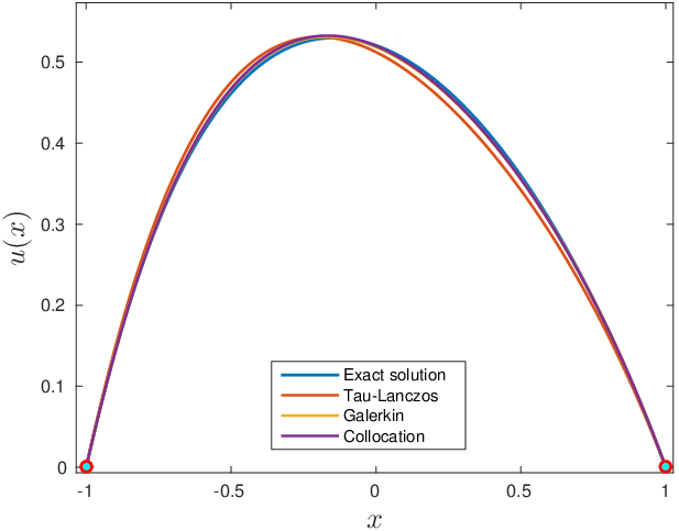
The comparison of three numerical solutions with the exact one (3.2) is shown in Figure 5. In this Figure 5 one can see that the collocation²⁹²⁹ 29 The advantage of the collocation approach for nonlinear (and variable coefficients) problems becomes even more flagrant. and Galerkin methods provide nearly identical³⁰³⁰ 30 With a little advantage towards the collocation method. However, this conclusion is not general at all. It is based only on this particular problem. numerical solutions which are closer to the exact solution than the prediction of the Tau method. However, in general the Author is impressed by the performance of spectral methods — with only five degrees of freedom $\{a_{k}\}_{k=0}^{4}$ we capture very well the global behaviour of the solution (3.2) in every point of the interval $\mathcal{I}$ . Perhaps, the last point has to be emphasized again: the (pseudo-)spectral methods provide the numerical value of the solution in the whole domain, not only in collocation or grid points.

Application to heat conduction

In this Section we show how to apply the Fourier-type spectral methods to simulate some simple and not so simple diffusion processes.

An elementary example

As the simplest example, consider the linear heat equation

u_{t}\ =\ \nu\,u_{xx}\,,\qquad x\ \in\ \mathds{R}\,,

(4.1)

completed with the initial condition

u(x,\,0)\ =\ u_{0}(x)\,.

We consider this equation on the whole line $\mathds{R}$ for the sake of simplicity. However, in silico it will be truncated to a periodic interval (in the example below it will be $\mathcal{I}\ =\ [-1,\,1]\,$ ). Let us apply the Fourier integral transform to the both sides of equation 4.1:

\dfrac{\mathrm{d}\hat{u}(k,\,t)}{\mathrm{d}\/t}\ =\ -\nu\,k^{2}\,\hat{u}(k,\,t)\,,

(4.2)

where the forward $\hat{u}(k,\,t)\ =\ \mathcal{F}\{u(x,\,t)\}$ and inverse $u(x,\,t)\ =\ \mathcal{F}^{-1}\{\hat{u}(k,\,t)\}$ integral Fourier transforms are defined below in (4.7) and (4.8) correspondingly. The transformed heat equation (4.2) can be regarded as a linear ODE. Its solution can be readily obtained:

\hat{u}(k,\,t)\ =\ \hat{u}_{0}(k)\,\mathrm{e}^{-\nu\,k^{2}\,t}\,,\qquad\hat{u}_{0}(k)\ =\ \mathcal{F}\{u_{0}(x)\}\,.

Consequently, we possess an analytical solution to the heat equation (4.1) in Fourier space. In order to obtain the solution in physical space, an inverse Fourier transform has to be computed. The exponential decay of Fourier coefficients $\hat{u}(k,\,t)$ (except the zero mode $k\ =\ 0$ ) ensures that the solution $u(x,\,t)$ becomes infinitely smooth $C^{\infty}$ for $t\ >\ 0\,$ . For example, the initial condition and corresponding solution at $t\ =\ T\ =\ 5\ {\sf s}$ are represented in Figure 6. The Matlab code used to generate Figure 6 is provided below as well.

⬇

1 l = 1.0; % half-length of the domain

2 N = 256; % number of Fourier modes

3 dx = 2*l/N; % distance between two collocation points

4 x = (1-N/2:N/2)*dx; % physical space discretization

5 nu = 0.01; % diffusion parameter

6 T = 5.0; % time where we compute the solution

8 dk = pi/l; % discretization step in Fourier space

9 k = [0:N/2 1-N/2:-1]*dk; % vector of wavenumbers

10 k2 = k.^2; % almost 2nd derivative in Fourier space

12 u0 = sech(10.0*x).^2; % initial condition

13 u0_hat = fft(u0); % Its Fourier transform

15 % and the solution at final time:

16 uT = real(ifft(exp(-nu*k2*T).*u0_hat));

A less elementary example

The numerical code above is based on the knowledge of the analytical solution to ODE (4.2) in the Fourier space. It is unnecessary to say that an analytical solution is available in very simple situations only. Consequently, we assume that the resulting ODE system in the physical (Fourier) space is formally solved (i.e. advanced in time) by the semigroup operator $\mathcal{S}(t)$ ( $\hat{\mathcal{S}}(t)\ \equiv\ \mathcal{F}\cdot\mathcal{S}(t)\cdot\mathcal{F}^{\,-1}$ correspondingly):

u(x,\,t)\ \equiv\ \mathcal{S}(t)\cdot\bigl[\,u_{0}(x)\,\bigr]\,.

In practice this semigroup operator is realized using numerical time-marching techniques described briefly in Appendix F. So, a more general Fourier spectral algorithm is

(1)

Decompose the initial condition:

$\hat{u}_{0}(k)\ =\ \mathcal{F}\bigl\{u_{0}(x)\bigr\}\,,$
(2)

Advance in time:

$\hat{u}_{k}(t)\ =\ \hat{\mathcal{S}}(t)\bigl[\,\hat{u}_{0}(k)\,\bigr]\,,$
(3)

Synthesize:

$u(x,\,t)\ =\ \mathcal{F}^{\,-1}\bigl\{\hat{u}_{k}(t)\bigr\}\,.$

This algorithm is based on the fact that the following diagram commutes:

A real-life example

In this Section we shall consider a realistic model (to be honest we take a slightly simplified version), which was proposed in [26] to predict heat and moisture transfer through the walls. This model is used in real-world Civil Engineering applications such as the code Domus. So, the model we consider in this Section reads (for simplicity we consider the 1D case):

	$\displaystyle\dfrac{\partial\theta}{\partial\/t}\$	$\displaystyle=\ \dfrac{\partial}{\partial\/x}\Bigl(\mathcal{D}_{\theta}\,\dfrac{\partial\theta}{\partial\/x}\ +\ \mathcal{D}_{T}\,\dfrac{\partial T}{\partial\/x}\Bigr)\,,$		(4.3)
	$\displaystyle\rho c_{m}\,\dfrac{\partial T}{\partial\/t}\$	$\displaystyle=\ -\dfrac{\partial q}{\partial\/x}\ -\ L(T)\cdot\dfrac{\partial j_{v}}{\partial\/x}\,,$		(4.4)

where $\theta$ is moisture volumetric content (i.e. moisture density) and $T$ is the temperature. The mass transport coefficients $\mathcal{D}_{\theta}(\theta,\,T)$ and $\mathcal{D}_{T}(\theta,\,T)$ may depend nonlinearly on the solution $\bigl(\theta(x,\,t),\,T(x,\,t)\bigr)$ . Here we assume for simplicity that the mass density $\rho$ and the specific moisture heat $c_{m}$ are some positive constants³¹³¹ 31 In more realistic modelling $c_{m}(\theta)$ depends also on the moisture density $\theta$ . It does not pose any problems to take it into account in the numerical scheme described in Section 4.. Finally, the heat flux $q$ and vapor flow $j_{v}$ can be expressed as

	$\displaystyle q\$	$\displaystyle=\ -\lambda(\theta,\,T)\,\dfrac{\partial T}{\partial\/x}\,,$
	$\displaystyle j_{v}\$	$\displaystyle=\ -\mathcal{V}_{\theta}(\theta,\,T)\,\dfrac{\partial\theta}{\partial\/x}\ -\ \mathcal{V}_{T}(\theta,\,T)\,\dfrac{\partial T}{\partial\/x}\,.$

In Fourier-type pseudo-spectral methods we usually work with Fourier coefficients. Consequently, we apply the Fourier transform to both sides of equations (4.3), (4.4):

	$\displaystyle\dfrac{\mathrm{d}\hat{\theta}}{\mathrm{d}\/t}\$	$\displaystyle=\ \mathrm{i}k\,\mathcal{F}\Bigl\{\mathcal{D}_{\theta}\,\dfrac{\partial\theta}{\partial\/x}\ +\ \mathcal{D}_{T}\,\dfrac{\partial T}{\partial\/x}\Bigr\}\,,$		(4.5)
	$\displaystyle\rho c_{m}\,\dfrac{\mathrm{d}\hat{T}}{\mathrm{d}\/t}\$	$\displaystyle=\ \mathrm{i}k\,\mathcal{F}\Bigl\{\lambda(\theta,\,T)\,\dfrac{\partial T}{\partial\/x}\Bigr\}\ -\ \mathcal{F}\Bigl\{L(T)\cdot\dfrac{\partial j_{v}}{\partial\/x}\Bigr\}\,,$		(4.6)

where we introduced some notations for the Fourier transform $\mathcal{F}(\cdot)$ :

\hat{\theta}(k,\,t)\ \mathop{\stackrel{{\scriptstyle\mathrm{def}}}{{:=}}}\ \mathcal{F}\Bigl\{\theta(x,\,t)\Bigr\}\ =\ \int_{-\infty}^{+\infty}\theta(x,\,t)\,\mathrm{e}^{\mathrm{i}kx}\;\mathrm{d}x\,,

(4.7)

where $k\in\mathds{R}$ is the wave number. Inversely we have

\theta(x,\,t)\ =\ \mathcal{F}^{\,-1}\Bigl\{\hat{\theta}(k,\,t)\Bigr\}\ =\ \frac{1}{2\pi}\,\int_{-\infty}^{+\infty}\hat{\theta}(k,\,t)\,\mathrm{e}^{-\mathrm{i}kx}\;\mathrm{d}k\,.

(4.8)

Now, system (4.5), (4.6) can be considered as a coupled nonlinear system of Ordinary Differential Equations (ODEs) (not PDEs!) for the Fourier coefficients of solutions $\bigl(\theta(x,\,t),\,T(x,\,t)\bigr)$ . The numerical methods for systems of ODEs will be explained in a separate course. As general fundamental references on this topic we can recommend [16, 17]. The Author even suggests to employ a well-documented ready-to-use ODE library such as [33], for example. Now we have to explain how to evaluate the right hand side of equations (4.5), (4.6) when only the Fourier coefficients are available. The recipe is very simple:

•

All linear operations (e.g. additions, subtractions, multiplication by a scalar) can be equally made in Fourier or in a real spaces. The choice has to be done in order to minimize the number of FFT operations

$\mathcal{F}\bigl\{\upalpha\theta\ +\ \upbeta T\bigr\}\ \equiv\ \upalpha\hat{\theta}\ +\ \upbeta\hat{T}$

•

All nonlinear products are made in the real space and then we transfer the result back to the Fourier space using one FFT, e.g.

\mathcal{F}\bigl\{\theta(x,\,t)\cdot T(x,\,t)\bigr\}\ =\ \mathcal{F}\Bigl\{\mathcal{F}^{\,-1}\bigl\{\hat{\theta}(k,\,t)\bigr\}\cdot\mathcal{F}^{\,-1}\bigl\{\hat{T}(k,\,t)\bigr\}\Bigr\}

•

All spatial derivatives are computed only in Fourier space, as

\dfrac{\partial^{n}}{\partial\/x^{n}}\bigl[\,\cdot\,\bigr]\quad\leftrightarrows\quad\mathcal{F}^{\,-1}\,\Bigl\{(\mathrm{i}k)^{n}\,\bigl[\,\cdot\,\bigr]\Bigr\}

The Reader can notice that above we used Fourier integrals. It comes from the mathematical tradition. In computer implementations one has to take a finite interval, periodize it and use direct and inverse Discrete Fourier Transforms (DFTs) instead of $\mathcal{F}\{\cdot\}$ and $\mathcal{F}^{\,-1}\{\cdot\}$ respectively.

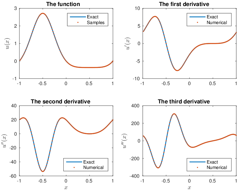
The computation of derivatives using the Fourier collocation spectral method is illustrated below on the following periodic function (with period $2$ ):

u(x)\ =\ \sin\bigl(\pi(x\ +\ 1)\bigr)\,\mathrm{e}^{\sin\left(\pi(x\ +\ 1)\right)}\,,\qquad x\ \in\ [-1,\,1]\,.

(4.9)

The first three derivatives of this function can be readily computed using any symbolic computation software (the Author used Maple):

u^{\,\prime}(x)\ =\ \pi\,\cos\bigl(\pi(x\ +\ 1)\bigr)\Bigl(1\ +\ \sin\bigl(\pi(x\ +\ 1)\bigr)\Bigr)\,\mathrm{e}^{\sin\left(\pi(x\ +\ 1)\right)}\,,

u^{\,\prime\prime}(x)\ =\ \pi^{2}\,\Bigl\{\cos^{2}\bigl(\pi(x\ +\ 1)\bigr)\,\Bigl(\sin\bigl(\pi(x\ +\ 1)\bigr)\ +\ 3\Bigr)\ -\ \sin\bigl(\pi(x\ +\ 1)\bigr)\ -\ 1\Bigr\}\,\mathrm{e}^{\sin\left(\pi(x\ +\ 1)\right)}\,,

u^{\,\prime\prime\prime}(x)\ =\ \pi^{3}\,\cos\bigl(\pi(x\ +\ 1)\bigr)\,\Bigl\{\cos^{2}\bigl(\pi(x\ +\ 1)\bigr)\,\Bigl(\sin\bigl(\pi(x\ +\ 1)\bigr)\ +\ 6\Bigr)\ -\ 7\,\sin\bigl(\pi(x\ +\ 1)\bigr)\ -\ 4\Bigr\}\,.

The expressions above are used to assess the accuracy of the computed approximations in collocation points. The analytical derivatives with computed ones (red dots) are shown in Figure 7 for $N\ =\ 128$ collocation points. To the graphical accuracy the results are indistinguishable. That is why we computed also the discrete $\ell_{\infty}$ norms to compute the relative errors:

\varepsilon_{N}^{(p)}\ =\ \frac{\lVert\,u_{\mathrm{num}}\ -\ u_{\mathrm{exact}}\,\rVert_{\infty}}{\lVert\,u_{\mathrm{exact}}(x_{i})\,\rVert_{\infty}}\,.

For $N\ =\ 32$ Fourier modes we obtain the following numerical results:

	$\displaystyle\varepsilon_{32}^{(1)}\$	$\displaystyle\approx\ 1.5\times 10^{-15}\,,$
	$\displaystyle\varepsilon_{32}^{(2)}\$	$\displaystyle\approx\ 8.4\times 10^{-15}\,,$
	$\displaystyle\varepsilon_{32}^{(3)}\$	$\displaystyle\approx\ 4.7\times 10^{-14}\,.$

The Matlab code used to generate these results and Figure 7 is provided below.

⬇

1 l = 1.0; % half-length of the domain

2 N = 128; % number of Fourier modes

3 dx = 2*l/N; % distance between two collocation points

4 x = (1-N/2:N/2)*dx; % physical space discretization

6 dk = pi/l;

7 k = [0:N/2 1-N/2:-1]*dk; % vector of wavenumbers

9 arg = pi*(x + 1);

10 sar = sin(arg);

11 car = cos(arg); car2 = car.*car;

12 esa = exp(sar);

13 u = sar.*esa;

14 uhat = fft(u);

16 % numerical derivatives:

17 up = real(ifft(1i*k.*uhat));

18 upp = real(ifft(-k.^2.*uhat));

19 uppp = real(ifft(-1i*k.^3.*uhat));

21 % exact derivatives:

22 pi2 = pi*pi; pi3 = pi2*pi;

23 u1 = pi*car.*(1 + sar).*esa;

24 u2 = pi2*(car2.*(sar + 3) - 1 - sar).*esa;

25 u3 = pi3*car.*(car2.*(sar + 6) - 4 - 7*sar).*esa;

Above we exploit the property that the Fourier transform is a ‘change a variables’ where the differentiation operator $\partial_{x}$ becomes diagonal.

Indications for further reading

If you got interested in the beautiful topic of pseudo-spectral methods, you can find more information in the following books:

•
The following book by N. Trefethen³²³² 32 Lloyd Nick Trefethen (1955 – 20..), an American/British numerical analyst. has two major advantages: (i) conciseness and (ii) collection of Matlab programs which comes along. I would recommend it as the first reading on pseudo-spectral methods. At least you will learn how to program efficiently in Matlab (or in Octave, Scilab, etc. ) [35]:
- –
  
  Trefethen, L. N. (2000). Spectral methods in MatLab. Society for Industrial and Applied Mathematics, Philadelphia, PA, USA.
•
The book by J. Boyd³³³³ 33 John Boyd (19.. – 20..), an American numerical analyst, meteorologist and occasional science fiction writer. is probably the most exhaustive one. It covers many topics and applications of spectral methods. The material is presented as a collection of tricks. For example, it is one of seldom books where (semi-)infinite domains and spherical geometries are covered. I am not sure that after reading this book you will know how to program the pseudo-spectral methods, but you will have a broad of view of possible issues and how to address them [2]:
- –
  
  Boyd, J. P. (2000). Chebyshev and Fourier Spectral Methods. (Dover Publications, New York) (2 ${}^{\mathrm{\small\textsf{nd}}}$ Ed.).
•
This book is probably my favourite one. It represents a good balance between the theory and practice and this book arose as an extended version of a previously published review paper. The present lecture notes were inspired in part on this book as well [11]:
- –
  
  Fornberg³⁴³⁴ 34 Bengt Fornberg (19.. – 20..), a Swedish/American numerical analyst., B. (1996). A practical guide to pseudospectral methods. Cambridge: Cambridge University Press.
•
The Author discovered this book only recently. So, he has still to read it, but from the first sight I can already recommend it:
- –
  
  Peyret, R. (2002). Spectral Methods for Incompressible Viscous Flow. Springer-Verlag New York Inc.
•
Finally, I discovered also these very clear and instructive Lecture notes [37]. Lectures were delivered in 2009 at the International Summer School ‘Modern Computational Science’ in Oldenburg, Germany. They can be freely downloaded at the following URL address:
- –
  
  http://www.staff.uni-oldenburg.de/hannes.uecker/pre/030-mcs-hu.pdf

In general, the Author’s suggestions (according to his personal taste and vision) for scientific literature and software are collected in a single document, which is continuously expanded and completed:

https://github.com/dutykh/libs/

Good luck and have a nice reading!

$\star$ $\star$ $\star$

Appendix A Some identities involving Tchebyshev polynomials

Tchebyshev polynomials $\{T_{n}(x)\}_{n=0}^{\infty}$ form a weighted orthogonal system on the segment $[-1,\,1]$ :

\langle\,T_{n},\,T_{m}\,\rangle\ \equiv\ \int_{-1}^{1}\,\frac{T_{n}(x)\cdot T_{m}(x)}{\sqrt{1\ -\ x^{2}}}\;\mathrm{d}x\ =\ \begin{cases}0,\quad m\ \neq\ n\,,\\ \pi,\quad m\ =\ n\ =\ 0\,,\\ \frac{\pi}{2},\quad m\ =\ n\ >\ 0\,.\end{cases}

The first few Tchebyshev polynomials are

	$\displaystyle T_{0}(x)\$	$\displaystyle=\ 1\,,$
	$\displaystyle T_{1}(x)\$	$\displaystyle=\ x\,,$
	$\displaystyle T_{2}(x)\$	$\displaystyle=\ 2\,x^{2}\ -\ 1\,,$
	$\displaystyle T_{3}(x)\$	$\displaystyle=\ 4\,x^{3}\ -\ 3\,x\,,$
	$\displaystyle T_{4}(x)\$	$\displaystyle=\ 8\,x^{4}\ -\ 8\,x^{2}\ +\ 1\,,$
	$\displaystyle T_{5}(x)\$	$\displaystyle=\ 16\,x^{5}\ -\ 20\,x^{3}\ +\ 5\,x\,.$

They are represented graphically in Figure 8. Higher order Tchebyshev polynomials can be constructed using the three-term recursion relation:

T_{n+1}(x)\ =\ 2\,x\,T_{n}(x)\ -\ T_{n-1}(x)\,.

The following Matlab code realizes this idea in practice:

⬇

1 function P = Chebyshev(n)

2 P = cell(n,1);

3 if (n == 1)

4 P{1} = 1;

5 return;

6 end % if ()

8 P{1} = 1;

9 P{2} = [1; 0];

10 for j=3:n

11 P{j} = [2*P{j-1}; 0];

12 P{j}(3:j) = P{j}(3:j) - P{j-2};

13 end % for j

15 end % Chebyshev()

Then, $n$ ${}^{\mathrm{\small\textsf{th}}}$ Tchebyshev polynomial can be evaluated using the standard Matlab’s function polyval(), e.g.

⬇

1 n = 5;

2 P = Chebyshev(n+1);

3 x = linspace(-1, 1, 1000);

4 Tn = polyval(P{n+1}, x);

There is an explicit expression for the $n$ ${}^{\mathrm{\small\textsf{th}}}$ polynomial:

T_{n}(x)\ =\ \cos\bigl(\,n\theta(x)\,\bigr)\,,\qquad\theta(x)\ \mathop{\stackrel{{\scriptstyle\mathrm{def}}}{{:=}}}\ \arccos x\,.

(A.1)

The first derivatives of Tchebyshev polynomials can be constructed recursively as well:

\frac{T_{n+1}^{\,\prime}(x)}{n\ +\ 1}\ =\ \frac{T_{n-1}^{\,\prime}(x)}{n\ -\ 1}\ +\ 2\,T_{n}(x)\,.

(A.2)

Otherwise, the first derivative $T_{n}^{\,\prime}(x)$ can be found from the following relation:

(1\ -\ x^{2})\,T_{n}^{\,\prime}(x)\ =\ -n\,x\,T_{n}(x)\ +\ n\,T_{n-1}(x)\,.

Tchebyshev polynomial $T_{n}(x)$ satisfies the following linear second order differential equation with non-constant coefficients:

(1\ -\ x^{2})\,T_{n}^{\,\prime\prime}\ -\ x\,T_{n}^{\,\prime}\ +\ n^{2}\,T_{n}\ =\ 0\,.

Finally, zeros of the $n$ ${}^{\mathrm{\small\textsf{th}}}$ Tchebyshev polynomial $T_{n}(x)$ are located at

x_{k}^{0}\ =\ \cos\,\Bigl(\,\frac{2k-1}{2n}\,\pi\,\Bigr)\,,\qquad k\ =\ 1,\,2,\,\ldots,\,n,

and extrema at

x_{k}^{\mathrm{ext}}\ =\ \cos\,\Bigl(\,\frac{\pi k}{n}\,\Bigr)\,,\qquad k\ =\ 0,\,1,\,\ldots,\,n\,.

When implementing Tchebyshev-type pseudo-spectral methods for nonlinear problems, one can use the expression of the product of two Tchebyshev polynomials in terms of higher and lower degree polynomials:

T_{m}(x)\,T_{n}(x)\ =\ \frac{1}{2}\;\bigl(\,T_{n+m}(x)\ +\ T_{n-m}(x)\,\bigr)\,,\qquad\forall n\ \geqslant\ m\ \geqslant\ 0\,.

To finish this Appendix we give the generating function for Tchebyshev polynomials:

\frac{1\ -\ x\,z}{1\ -\ 2\,x\,z\ +\ z^{2}}\ =\ \sum_{n\,=\,0}^{\infty}\,T_{n}(x)\,z^{n}\,.

In order to satisfy the requirement (2) from Section 2.1, we provide here the relations which allow to re-express the derivatives of the Tchebyshev expansion in terms of Tchebyshev polynomials again. Namely, consider a truncated series expansion of a function $u(x)$ in Tchebyshev polynomials:

u(x)\ =\ \sum_{k\,=\,0}^{N}v_{k}\,T_{k}(x)\,.

Imagine that we want to compute the first derivative of the expansion above (it is always possible, since the sum is finite and we can differentiate term by term):

u^{\,\prime}(x)\ =\ \sum_{k\,=\,0}^{N}v_{k}\,\dfrac{\mathrm{d}T_{k}(x)}{\mathrm{d}\/x}\,.

Now we re-expand the derivative $u^{\,\prime}(x)$ in the same basis functions:

u^{\,\prime}(x)\ =\ \sum_{k\,=\,0}^{N}v_{k}^{\,\prime}\,T_{k}(x)\,.

The main question is how to re-express the coefficients $\{v_{k}^{\,\prime}\}_{k=0}^{N}$ in terms of coefficients $\{v_{k}\}_{k=0}^{N}\,$ ? This goal is achieved using basically the recurrence relation (A.2) (even if it does not jump into the eyes). Thanks to it we have an explicit relation between the coefficients:

v_{k}^{\,\prime}\ =\ \frac{2}{\delta_{k}}\;\sum_{\stackrel{{\scriptstyle j\,=\,k+1}}{{j+k\ \mathrm{odd}}}}^{N}\,j\,v_{j}\,,\qquad j\ =\ 0,\,1,\,\ldots,N-1\,,

where

\delta_{k}\ =\ \begin{cases}\ 2,&\ k\,=\,0\,,\\ \ 0,&\ k\,\neq\,0\,.\end{cases}

A similar ‘trick’ can be made for the 2 ${}^{\mathrm{\small\textsf{nd}}}$ derivative as well:

u^{\,\prime\prime}(x)\ =\ \sum_{k=0}^{N}v_{k}\,\dfrac{\mathrm{d}^{2}T_{k}(x)}{\mathrm{d}\/x^{2}}\ =\ \sum_{k=0}^{N}v_{k}^{\,\prime\prime}\,T_{k}(x)\,.

The connection between coefficients $\{v_{k}^{\,\prime\prime}\}_{k=0}^{N}$ and $\{v_{k}\}_{k=0}^{N}$ is given by the following explicit formula:

v_{k}^{\,\prime\prime}\ =\ \frac{1}{\delta_{k}}\;\sum_{\stackrel{{\scriptstyle j=k+2}}{{j+k\ \mathrm{even}}}}^{N}\,j\,(j^{2}\ -\ k^{2})\,v_{j}\,,\qquad j\ =\ 0,\,1,\,\ldots,N-2\,.

Finally, in order to construct the spectral coefficients for the $n$ ${}^{\mathrm{\small\textsf{th}}}$ derivative, one can use the following recurrence relation (also stemming from (A.2)):

\delta_{k-1}\,v_{k-1}^{(n)}\ =\ v_{k+1}^{(n)}\ +\ 2\,k\,v_{k}^{(n-1)}\,,\qquad k\ \geqslant\ 1\,,

which has to be completed by starting value $v_{N}^{\,\prime}\ \equiv\ 0\,$ .

Remark 8.

Similar identities exist for the family of Jacobi polynomials $\mathcal{P}_{n}^{\,\upalpha,\,\upbeta}(x)$ as well. However, they are more complicated due to the presence of two arbitrary parameters $\upalpha,\,\upbeta\ >\ -1$ . The family of Tchebyshev polynomials is a particular case of Jacobi polynomials when $\upalpha\ =\ \upbeta\ =\ -\frac{1}{2}$ .

Compositions of Tchebyshev polynomials

We would like to show here another interesting formula involving Tchebyshev polynomials:

Theorem 2 (Composition formula).

If $T_{n}(x)$ and $T_{m}(x)$ are Tchebyshev polynomials ( $m,n\ \geqslant\ 0$ ), then

\bigl(T_{m}\circ T_{n}\bigr)\,(x)\ \equiv\ T_{m}\bigl(T_{n}\,(x)\bigr)\ =\ T_{mn}(x)\,.

(A.3)

Proof.

An eleven (!) pages combinatorial proof of this result can be found in [1]. Here we shall prove the composition formula (A.3) in one line by using some rudiments of complex variables. Let us introduce the variable $z\ \mathop{\stackrel{{\scriptstyle\mathrm{def}}}{{:=}}}\ \mathrm{e}^{\mathrm{i}\theta}\ \in\ \circlearrowleft$ ³⁵³⁵ 35 Symbol $\circlearrowleft$ denotes the unit circle $\mathcal{S}_{1}(\boldsymbol{0})$ on the complex plane $\mathds{C}$ . such that

x\ =\ \frac{1}{2}\;\Bigl(z\ +\ \frac{1}{z}\Bigr)\,\quad\leftrightarrows\quad x\ =\ \cos\theta\,.

Then, by (A.1) we have a complex representation of the $n$ ${}^{\mathrm{\small\textsf{th}}}$ Tchebyshev polynomial:

T_{n}\,(x)\ \equiv\ T_{n}\Bigl[{\textstyle{1\over 2}}\,\bigl(z\ +\ z^{\,-1}\bigr)\Bigr]\ =\ \frac{1}{2}\;\Bigl(z^{\,n}\ +\ \frac{1}{z^{\,n}}\Bigr)\,.

Now, we have all the elements to show the main result:

T_{m}\biggl[\,T_{n}\Bigl({\textstyle{1\over 2}}\,\bigl(z\ +\ z^{\,-1}\bigr)\Bigr)\,\biggr]\ =\ T_{m}\Bigl[\,{\textstyle{1\over 2}}\,\bigl(z^{\,n}\ +\ z^{\,-n}\bigr)\Bigr]\ =\ \frac{1}{2}\;\Bigl((z^{\,n})^{\,m}\ +\ \frac{1}{(z^{\,n})^{\,m}}\Bigr)\ =\\ \frac{1}{2}\;\Bigl(z^{\,mn}\ +\ \frac{1}{z^{\,mn}}\Bigr)=\ T_{mn}\Bigl[{\textstyle{1\over 2}}\,\bigl(z\ +\ z^{\,-1}\bigr)\Bigr]\ \equiv\ T_{mn}\,(x)\,.

∎

Appendix B Trefftz method

In this Appendix I would like to give the flavour of the so-called Trefftz³⁶³⁶ 36 Erich Emmanuel Trefftz (1888 – 1937), a German Mathematician and Mechanical Engineer. methods, which remain essentially unknown/forgotten nowadays. These methods belong to boundary-type solution procedures. Below I shall quote a Professor³⁷³⁷ 37 His/Her identity will be hidden in order to avoid any kind of diplomatic incidents. from Laboratoire Jacques-Louis Lions (LJLL) at Paris 6 Pierre and Marie Curie University, who makes interesting comments about the knowledge of Trefftz methods in French Applied Mathematics community (the original language and orthography are conserved):

[ …] Sinon j’ai moi aussi fait une petite enquête, à la suite de laquelle il apparaît que personne ne connait Trefftz chez les matheux de Paris 6, hormis Nataf qui en a entendu parler pendant son DEA en méca !!!

Trefftz est un grand oublié car son papier est vraiment extrêmement intéressant, encore plus si tu te rends compte qu’il produit en fait une estimation a posteriori (ça doit même être la première). En revanche je me suis aussi persuadé que les méthodes de Trefftz végètent chez les mécano. [ …]

So, the situation is rather sad. Fortunately this method continued to live in the Mechanical Engineering community who preserved it for future generations.

In the exposition below we shall follow an excellent review paper [23]. More precisely we describe the so-called indirect Trefftz method, which was proposed originally by E. Trefftz (1926) in [36]. There are also direct Trefftz methods proposed some sixty years later in [4]. They are much closer to the Boundary Integral Equation Methods (BIEM) and will not be covered here. Interested readers can refer to [23].

Consider a (compact) domain $\Omega\ \subseteq\ \mathds{R}^{d}$ , $d\ \geqslant\ 2$ and a (scalar) equation on it (see Figure 9 for an illustration):

\mathscr{L}u\ =\ 0\,.

(B.1)

You can think, for example, that $\mathscr{L}\ =\ -\boldsymbol{\nabla}^{2}\ =\ -\sum_{i\,=\,1}^{d}\,\dfrac{\partial^{2}}{\partial\/x_{i}^{2}}$ is the Laplace³⁸³⁸ 38 Pierre–Simon de Laplace (1749 – 1827) is a French Mathematician whose works were greatly disregarded during his times. The understanding of their importance came much later (il vaut mieux tard que jamais ☺). operator. Equation (B.1) has to be completed by appropriate boundary conditions:

\mathscr{B}\,u\ =\ u^{\circ}\,,\qquad\boldsymbol{x}\ \in\ \partial\,\Omega\,,

(B.2)

where $u^{\circ}$ is the boundary data (solution value or its flux) and $\mathscr{B}$ is an operator depending on the type of boundary conditions in use. For example, in the case of Laplace equation the following choices are popular:

Dirichlet:: $\mathscr{B}\ \mathop{\stackrel{{\scriptstyle\mathrm{def}}}{{:=}}}\ \mathbb{I}$ (Identity operator, i.e. $\mathbb{I}u\ \equiv\ u$ ); in this case the solution value is prescribed on the boundary.
Neumann:: $\mathscr{B}\ \mathop{\stackrel{{\scriptstyle\mathrm{def}}}{{:=}}}\ \dfrac{\partial}{\partial\/n}\ \equiv\ \boldsymbol{n}\boldsymbol{\cdot}\boldsymbol{\nabla}\ =\ \sum_{i\,=\,1}^{d}\,n_{i}\cdot\dfrac{\partial}{\partial\/x_{i}}$ (Normal derivative, $\boldsymbol{n}$ being the exterior normal to $\partial\,\Omega$ ); physically it corresponds to the prescribed flux through the boundary.
Robin:: $\mathscr{B}\ \mathop{\stackrel{{\scriptstyle\mathrm{def}}}{{:=}}}\ \upalpha\,\mathbb{I}\ +\ \upbeta\;\dfrac{\partial}{\partial\/n}$ , where $\upalpha,\,\upbeta\ \in\ \mathds{R}$ are some parameters; this case is a mixture of two previous situations. It arises in some problems as well (see e.g. [5] for the heat conduction problem in thin liquid films).

Notice, that the boundary $\partial\,\Omega$ can be divided in some sub-domains where a different boundary condition is imposed:

\partial\,\Omega\ =\ \Gamma_{1}\ \cup\ \Gamma_{2}\ \cup\ \ldots\ \cup\ \Gamma_{n}\,\qquad\mu_{d}\,\Bigl(\Gamma_{i}\ \cap\ \Gamma_{j}\Bigr)\ =\ 0\,,\quad 1\ \leqslant\ i\ <\ j\ \leqslant\ n\,,

where $\mu_{d}$ is the Lebesgue measure in $\mathds{R}^{d}$ .

In the indirect Trefftz method the numerical solution is sought as a linear combination of $\mathbb{T}$ -complete functions $\bigl\{\phi_{k}(\boldsymbol{x})\bigr\}_{k\,=\,1}^{n}$ [20], which satisfy exactly the governing equation (B.1):

u_{n}(\boldsymbol{x})\ =\ \sum_{k\,=\,1}^{n}\,v_{k}\,\phi_{k}(\boldsymbol{x})\,.

(B.3)

For example, for the Laplace equation in $\mathds{R}^{2}$ the $\mathbb{T}$ -complete set of functions is [19] $\bigl\{r^{\,k}\,\mathrm{e}^{\,\mathrm{i}k\theta}\bigr\}_{k=0}^{\infty}$ , where $(r,\,\theta)$ are polar coordinates³⁹³⁹ 39 $r\ =\ \sqrt{x^{2}\ +\ y^{2}}$ , $\quad\theta\ =\ \arctan\,\dfrac{y}{x}\,,\quad$ with $\arctan\,(\pm\infty)\ =\ \pm\dfrac{\pi}{2}\,$ . on plane. The coefficients $\{v_{k}\}_{k=1}^{n}$ are to be determined. To achieve this goal the approximate solution (B.3) is substituted into the boundary conditions (B.2) to form the residual:

\mathscr{R}[u_{n}]\ =\ \mathscr{B}\,u_{n}\ -\ u^{\circ}\,.

If the residual $\mathscr{R}[u_{n}]$ is equal identically to zero on the boundary $\partial\,\Omega$ , then we found the exact solution (we are lucky!). Otherwise (we are unlucky and in Numerical Analysis it happens more often), the residual has to be minimized. Very often the boundary operator $\mathscr{B}$ is linear and we can write:

\mathscr{R}[u_{n}]\ =\ \sum_{k\,=\,1}^{n}\,v_{k}\,\mathscr{B}\,\phi_{k}(\boldsymbol{x})\ -\ u^{\circ}\,.

So, we can apply now the collocation, Galerkin or least square methods to determine the coefficients $\{v_{k}\}_{k\,=\,1}^{n}$ . These procedures were explained above.

Remark 9.

Suppose that a $\mathbb{T}$ -complete set of functions for equation (B.1) is unknown. However, there is a way to overcome this difficulty if we know the Green⁴⁰⁴⁰ 40 George Green (1793 – 1841), a British Mathematician who made great contributions to the Mathematical Physics and PDEs. function⁴¹⁴¹ 41 The Green function is named after George Green (see the footnote above), but the notion of this function can be already found first in the works of Laplace, then in the works of Poisson. As I said, the works of Laplace were essentially disregarded by his “colleagues”. Poisson was luckier in this respect. He is also known for (mis)using his administrative resource in order to delay (just for a couple of decades, nothing serious ☺) the publication of his competitors, e.g. the young (at that time) Cauchy. $\mathcal{G}(\boldsymbol{x};\,Q)$ , $\boldsymbol{x}\in\ \Omega$ for our equation (B.1), i.e.

\mathscr{L}\,\mathcal{G}\ =\ \delta\bigl(\boldsymbol{x}\ -\ Q\bigr)\,,\qquad\boldsymbol{x}\ \in\ \Omega\,,\qquad Q\ \in\ \mathds{R}^{d}\,.

where $\delta(\boldsymbol{x})$ is the singular Dirac measure. Notice that point $Q$ can be inside or outside of domain $\Omega$ , where the problem is defined. Then, we can seek for an approximate solution $u_{n}(\boldsymbol{x})$ as a linear combination of Green functions:

u_{n}(\boldsymbol{x})\ =\ \sum_{k\,=\,1}^{n}\,v_{k}\,\mathcal{G}_{k}(\boldsymbol{x};\,Q_{k})\,,

where the points $\bigl\{Q_{k}\bigr\}_{k=1}^{n}$ are distributed outside of the computational domain $\Omega$ in order to avoid the singularities. This method is schematically illustrated in Figure 9. The accuracy of this approach depends naturally on the distribution of points $\bigl\{Q_{k}\bigr\}_{k=1}^{n}$ . To Author’s knowledge there exist no theoretical indications for the optimal distribution (as it is the case of Tchebyshev nodes on a segment). So, it remains mainly an experimental area of the research.

Conclusions.

In the indirect Trefftz methods (historically, the original one) the problem solution is sought as a linear combination of the functions, which satisfy the governing equation identically. Then, the unknown coefficients are chosen so that the approximate solution satisfies the boundary condition(s) as well. It can be done by means of collocation, Galerkin or least square procedures. The main advantage of Trefftz methods is that it allows to reduce problem’s dimension by one (i.e. 3D $\rightsquigarrow$ 2D and 2D $\rightsquigarrow$ 1D), since the residual $\mathscr{R}[u_{n}]$ is minimized on the domain boundary $\partial\,\Omega\ \subseteq\ \mathds{R}^{d-1}$ . Readers who are interested in the application of Trefftz methods to their problems should refer to [23] and references therein.

Appendix C A brief history of diffusion in Physics

Since the main focus of the PhD school is set on the diffusion processes (molecular diffusion, heat and moisture conduction through the walls, etc. ), it is desirable to explain how this research started and why the diffusion is generally modeled by parabolic PDEs [10]. The historic part of this Appendix is partially based on [29].

Firs of all, let us make a general, perhaps surprising, remark, which is based on the analysis of historical investigations: understanding the microscopic world is not compulsory to propose a reliable macroscopic law. Indeed, Fourier did not know anything about the nature of heat, Ohm⁴²⁴² 42 Georg Simon Ohm (1789 – 1854) was a German Physicist. about the nature of electricity, Fick⁴³⁴³ 43 Adolf Eugen Fick (1829 – 1901) was a German physician and physiologist. about salt solutions and Darcy⁴⁴⁴⁴ 44 Henry Darcy (1803 - 1858) was a French engineer in Hydraulics. about the structure of porosity and water therein. In cases of the diffusion, the bridge between microscopic and macroscopic worlds was built by A. Einstein⁴⁵⁴⁵ 45 Albert Einstein (1879 – 1955) was a German theoretical Physicist. This personality does not need to be introduced. in 1905. Namely, he expressed a macroscopic quantity — the diffusion coefficient — in terms of microscopic data (this result will be given below). In general, 1905 was Annus Mirabilis⁴⁶⁴⁶ 46 Annus Mirabilis comes from Latin and stands for “extraordinary year” in English or “Wunderjahr” in German. for A. Einstein. During this year he published four papers in Annalen der Physik whose aftermath was prodigious.

The first scientific study of diffusion was performed by a Scottish chemist Thomas Graham (1805 – 1869). His research on diffusion was conducted between 1828 and 1833. Here we quote his first paper:

[ …] the experimental information we possess on the subject amounts to little more than the well established fact, that gases of different nature, when brought into contact, do not arrange themselves according to their density, the heaviest undermost, and the lighter uppermost, but they spontaneously diffuse, mutually and equally, through each other, and so remain in the intimate state of mixture for any length of time.

In 1867 James Maxwell⁴⁷⁴⁷ 47 James Clerk Maxwell (1831 – 1879) was a Scottish Physicist, famous for Maxwell equations. estimated the diffusion coefficient of $\mathrm{CO}_{2}$ in the air using the results (measurements) of Graham. The resulting number was obtained within 5% accuracy. It is pretty impressive.

A. Fick⁴⁸⁴⁸ 48 Adolf Fick was the author of the first treatise of Die medizinische Physik (Medical Physics) (1856) where he discussed biophysical problems, such as the mixing of air in the lungs, the work of the heart, the heat economy of the human body, the mechanics of muscular contraction, the hydrodynamics of blood circulation, etc. hold a chair of physiology in Würzburg for 31 years. His main contributions to Physics were made during a few years around 1855. When he was 26 years old he published a paper on diffusion establishing the now classical Fick’s diffusion law. Fick did not realize that dissolution and diffusion processes result from the movement of separate entities of salt and water. He deduced the quantitative law proceeding in analogy with the work of J. Fourier [12] who modeled the heat conduction:

[ …] It was quite natural to suppose that this law for diffusion of a salt in its solvent must be identical with that according to which the diffusion of heat in a conducting body takes place; upon this law Fourier founded his celebrated theory of heat, and it is the same that Ohm applied [ …] to the conduction of electricity [ …] according to this law, the transfer of salt and water occurring in a unit of time between two elements of space filled with two different solutions of the same salt, must be, ceteris partibus, directly proportional to the difference of concentrations, and inversely proportional to the distance of the elements from one another.

Going along this analogy, Fick assumed that the flux of matter is proportional to its concentration gradient with a proportionality factor $\kappa$ , which he called “a constant dependent upon the nature of the substances”. Actually, Fick made an error in (minus) sign which introduces the anti-diffusion and leads to an ill-posed problem. This error was not a source of difficulty for Fick since he analyzed only steady states in accordance with available experimental conditions at that time.

The fundamental article [8] devoted to the study of Brownian⁴⁹⁴⁹ 49 Robert Brown (1773 – 1858) was a Scottish Botanist. motion and entitled “On the Motion of Small Particles Suspended in a Stationary Liquid, as Required by the Molecular Kinetic Theory of Heat” by Einstein was published on 18 ${}^{\mathrm{\small\textsf{th}}}$ July 1905 in Annalen der Physik. By the way, it is the most cited Einstein’s paper among four works published during his Annus Mirabilis. This manuscript is of capital interest to us as well. Let us quote a paragraph from [8]:

In this paper it will be shown that, according to the molecular kinetic theory of heat, bodies of a microscopically visible size suspended in liquids must, as a result of thermal molecular motions, perform motions of such magnitudes that they can be easily observed with a microscope. It is possible that the motions to be discussed here are identical with so-called Brownian molecular motion; however, the data available to me on the latter are so imprecise that I could not form a judgment on the question [ …]

Einstein was the first to understand that the main quantity of interest is the mean square displacement $\langle X^{2}(t)\rangle$ and not the average velocity of particles. Taking into account the discontinuous nature of particle trajectories, the velocity is meaningless.

Before publication of [8] atoms in Physics were considered as a useful, but purely theoretical concept. Their reality was seriously debated. W. Ostwald⁵⁰⁵⁰ 50 Friedrich Wilhelm Ostwald (1853 – 1932) was a Latvian Chemist. He received a Nobel prize in Chemistry in 1909 for his works on catalysis., one of the leaders of the anti-atom school, later told A. Sommerfeld⁵¹⁵¹ 51 Arnold Johannes Wilhelm Sommerfeld (1868 – 1951) was a German theoretical Physicist. He served as the PhD advisor for several Nobel prize winners. that he had been convinced of the existence of atoms by Einstein’s complete explanation of Brownian motion.

Without knowing it, Einstein in answered a question posed the same year by K. Pearson⁵²⁵² 52 Karl Pearson (1857 – 1936) was an English Statistician. in a Letter published in Nature [28]:

Can any of your readers refer me to a work wherein I should find a solution of the following problem, or failing the knowledge of any existing solution provide me with an original one? I should be extremely grateful for aid in the matter.

A man starts from a point $O$ and walks $\ell$ yards in a straight line; he then turns through any angle whatever and walks another $\ell$ yards in a second straight line. He repeats this process $n$ times. I require the probability that after these $n$ stretches he is at a distance between $r$ and $r\ +\ \mathrm{d}r$ from his starting point, $O$ .

The problem is one of considerable interest, but I have only succeeded in obtaining an integrated solution for two stretches. I think, however, that a solution ought to be found, if only in the form of a series in powers of $\dfrac{1}{n}$ , when $n$ is large.

The expression “random walk” was probably coined in Pearson’s Letter [28].

Let us follow Einstein’s study of the Brownian motion. Consider a long thin tube filled with water (it allows us to consider only one spatial dimension). At the initial time $t\ =\ 0$ we inject a unit amount of ink at $x\ =\ 0$ . Let $u(x,\,t)$ denote the density of ink particles in location $x\ \in\ \mathds{R}$ and at time $t\ \geqslant\ 0$ . So, initially we have

u(x,\,0)\ =\ \delta(x)\,,

(C.1)

where $\delta(x)$ is the Dirac distribution centered at zero.

Then, suppose that the probability density of the event that an ink particle moves from $x$ to $x+\Delta x$ in a small time $\Delta t$ is $\rho(\Delta x,\,\Delta t)$ . Then, we have

u\,(x,\,t\ +\ \Delta t)\ =\ \int_{-\infty}^{+\infty}\,u(x-\Delta x,\,t)\,\rho(\Delta x,\,\Delta t)\;\mathrm{d}\bigl(\Delta x\bigr)\,.

Assuming that solution $u(x,\,t)$ is smooth, we can apply the Taylor⁵³⁵³ 53 Brook Taylor (1685 – 1731) was an English Mathematician. formula:

u\,(x,\,t\ +\ \Delta t)\ =\ \int_{-\infty}^{+\infty}\,\Bigl(u\ -\ u_{x}\cdot\Delta x\ +\ \frac{1}{2}\,u_{xx}\cdot\bigl(\Delta x\bigr)^{2}\ +\ \cdots\Bigr)\,\rho(\Delta x,\,\Delta t)\;\mathrm{d}\bigl(\Delta x\bigr)\,.

(C.2)

Now let us recall that $\rho$ is a Probability Density Function (PDF). Thus,

Normalisation:

$\int_{-\infty}^{+\infty}\,\rho(\Delta x,\,\Delta t)\;\mathrm{d}\bigl(\Delta x\bigr)\ =\ 1$

Symmetry:

we can assume that the diffusion process is symmetric in space, i.e.

\rho(\Delta x,\,\Delta t)\ =\ \rho(-\Delta x,\,\Delta t)\,,\qquad\forall\Delta x,\ \Delta t\ \geqslant\ 0\,.

Consequently,

\int_{-\infty}^{+\infty}\,\Delta x\,\rho(\Delta x,\,\Delta t)\;\mathrm{d}\bigl(\Delta x\bigr)\ =\ 0\,.

Variance:

We can also assume that the variance if finite and Einstein assumed additionally that the variance is linear in $\Delta t$ :

\int_{-\infty}^{+\infty}\,\bigl(\Delta x\bigr)^{2}\,\rho(\Delta x,\,\Delta t)\;\mathrm{d}\bigl(\Delta x\bigr)\ =\ \mathcal{D}\Delta t\,,

where $\mathcal{D}\ >\ 0$ is the so-called diffusion constant.

By incorporating these results into equation (C.2) and rearranging the terms, it becomes

\frac{u(x,\,t+\Delta t)\ -\ u(x,\,t)}{\Delta t}\ =\ \frac{1}{2}\,\mathcal{D}\,u_{xx}\,(x,\,t)\ +\ \cdots\,.

Taking the limit $\Delta t\ \to\ 0$ we obtain straightforwardly

u_{t}\ =\ \frac{1}{2}\,\mathcal{D}\,u_{xx}\,.

(C.3)

The Initial Value Problem (C.1) for this linear parabolic equation (C.3) can be solved exactly:

u(x,\,t)\ =\ \frac{1}{\sqrt{2\pi\mathcal{D}t}}\,\mathrm{e}^{-\frac{x^{2}}{2\mathcal{D}t}}\,.

The last solution is also known as the Green function.

However, the main result of Einstein’s paper [8] is the following formula:

\mathcal{D}\ =\ \frac{RT}{fN_{a}}\,,

(C.4)

where

$R$ :: the ideal gas constant, i.e. $R\ \approx\ 8.3144598$ $\dfrac{\mathsf{J}}{\mathsf{K}\cdot\mathsf{mol}}$
$T$ :: the absolute temperature
$f$ :: the friction coefficient
$N_{a}$ :: Avogadro’s⁵⁴⁵⁴ 54 Lorenzo Romano Amedeo Carlo Avogadro di Quaregna e di Cerreto (1776 – 1856) was an Italian scientist. number, i.e. $N_{a}\ \approx\ 6.022140857$ $\mathsf{mol}^{-1}$

Formula (C.4) along with the observation of the Brownian motion enabled J. Perrin⁵⁵⁵⁵ 55 Jean Baptiste Perrin (1870 – 1942) was a French Physicist who was honoured with the Nobel prize in Physics in 1926 for the confirmation of the atomic nature of matter (through the observation of Brownian motion). to produce the first historical estimation of Avogadro’s constant $N_{a}\ \approx\ 6$ $\mathsf{mol}^{-1}$ .

Exercise 1.

Read a fascinating paper by A. Einstein on the Hydrodynamics of tea leaves [9]. By the way, the Author attests that Tea is very stimulating for intellectual activities. ☺

Appendix D Monte–Carlo approach to the diffusion simulation

From considering the history and physical modelling of Brownian motion we naturally come to the numerical simulation of parabolic PDEs using stochastic processes. It falls into the large class of Monte–Carlo and quasi-Monte–Carlo methods [3]. They are based on the so-called Law of large numbers, which can be informally stated⁵⁶⁵⁶ 56 We choose this particular form, since it is suitable for our exposition. as

\lim_{N\to+\infty}\frac{1}{N}\sum_{n\,=\,1}^{N}g(\xi_{n})\ =\ \mathbb{E}\,[g(\xi)]\,,

where $\xi_{n}$ are independent, identically distributed random variables and $g(\cdot)$ is a real-valued continuous function. Here $\mathbb{E}\,[\cdot]$ stands for the mathematical expectation and the convergence is understood in the sense convergence in probability distribution⁵⁷⁵⁷ 57 A sequence of random variables $\{\xi_{n}\}_{n=1}^{\infty}$ converges in probability distribution towards the random variable $\xi$ if for $\forall\,\varepsilon\ >\ 0$ $\lim_{n\to\ \infty}\mathbb{P}\bigl\{\lvert\,\xi_{n}\ -\ \xi\,\rvert\ \geqslant\ \varepsilon\bigr\}\ =\ 0\,.$ This fact can be denoted as $\xi_{n}\ \stackrel{{\scriptstyle\mathbb{P}}}{{\rightsquigarrow}}\ \xi$ .. The proof is based on the Tchebyshev inequality in Probabilities, but we do not enter into these details. The main advantages of Monte–Carlo methods are

•

Simplicity of implementation
•

Independent of the problem dimension (they do not suffer of the curse of dimensionality)

On the other hand, the convergence rate is given by the Central Limit Theorem [22] and it is rather slow, i.e. $\mathcal{O}(N^{\,-1/2})$ , even if some acceleration is possible thanks to some adaptive procedures [25] (such as low-discrepancy sequences, variance reduction and multi-level methods). The large deviation theory guarantees that the probability of falling out of a fixed tolerance interval decays exponentially fast.

To the Author knowledge, the method we are going to describe below was first proposed by R. Feynman⁵⁸⁵⁸ 58 Richard Phillips Feynman (1918 – 1988) was an American theoretical Physicist. Nobel Prize in Physics (1965) and Author’s hero. Please, do not hesitate to read any of his books! in order to solve numerically the linear Schrödinger⁵⁹⁵⁹ 59 Erwin Rudolf Josef Alexander Schrödinger (1887 – 1961) was an Austrian theoretical Physicist. Nobel prize in Physics (1933) for the formulation of what is known now as the Schrödinger equation. equation in 1940s. In fact, he noticed that the Schrödinger equation can be solved by a kind of average over trajectories. This observation led him to a far-reaching reformulation of the quantum theory in terms of path integrals. Upon learning Feynman’s ideas, M. Kac⁶⁰⁶⁰ 60 Mark Kac (1914 – 1984) was a Polish mathematician who studied in Lviv University, Ukraine and immigrated later to USA. (Feynman’s colleague at Cornell University) understood that a similar method can work for the heat equation as well. Later it became Feynman–Kac method. Unfortunately, this method is not implemented in any commercial software (for PDEs, the financial industry is using these methods since many decades) and it is not described in classical textbooks on PDEs and in the books on numerical methods for PDEs.

Consider first the following simple heat equation:

u_{t}\ =\ \frac{1}{2}\;u_{xx}\ -\ V(x)\cdot u\,,

(D.1)

where $V(x)$ is a function representing the amount of external cooling (if $V(x)\geqslant 0$ , and external heating if $V(x)<0$ , but we do not consider this case) at point $x$ . Then, we have the following

Theorem 3 (Feynman–Kac formula).

Let $V(x)$ be a non-negative continuous function and let $u_{0}(x)$ be bounded and continuous. Suppose that $u(x,\,t)$ is a bounded function that satisfies equation (D.1) along with the initial condition

u(x,\,0)\ =\ u_{0}(x)\,,

(D.2)

then,

u(x,\,t)\ =\ \mathbb{E}\,\biggl[\,\exp\Bigl\{-\int_{0}^{t}V\bigl(\mathcal{W}_{s}\bigr)\;\mathrm{d}s\Bigr\}\;u_{0}\bigl(\mathcal{W}_{t}\bigr)\,\biggr]\,,

(D.3)

where $\{\mathcal{W}_{t}\}_{t\,\geqslant\,0}$ is a Brownian motion starting at $x$ .

We have to define rigorously also what the Brownian motion is:

Definition 1 (Brownian motion).

A real-valued stochastic process $t\ \mapsto\ \mathcal{W}(t)$ (or a random curve) is called a Brownian motion (or Wiener process) if

(1)

Almost surely $\mathcal{W}(0)\ =\ 0$
(2)

$\mathcal{W}(t)\ -\ \mathcal{W}(s)\ \thicksim\ \mathscr{N}(0,\,t\ -\ s)\ \equiv\ \sqrt{t\ -\ s}\,\mathscr{N}(0,\,1)$ , $\quad\forall t\ \geqslant\ s\ \geqslant\ 0$
(3)

For any instances of time $v\ >\ u\ >\ t\ >\ s\ \geqslant\ 0$ the increments $\mathcal{W}(v)-\mathcal{W}(u)$ and $\mathcal{W}(t)-\mathcal{W}(s)$ are independent random variables.

In particular, from point (2) by choosing $s=0$ it follows directly that

\mathbb{E}\bigl[\mathcal{W}(t)\bigr]\ =\ 0,\qquad\mathbb{E}\bigl[\mathcal{W}^{\,2}(t)\bigr]\ =\ t\,.

More informally we can say that the Brownian motion is a continuous random curve with the largest possible amount of randomness.

The Theorem above can be proved even under more general assumptions, but the formulation given above suffices for most practical situations. For instance, the functions $V(x)$ and $u_{0}(x)$ may have isolated discontinuities and the Feynman–Kac formula will be still valid. Another interesting corollary of Feynman–Kac’s formula is the uniqueness of solutions to the Initial Value Problem (IVP) (D.1):

Corollary 1.

Under the assumptions of Theorem 3, there is at most one solution to the heat equation (D.1), which satisfies the initial condition (D.2). Namely, it is given by Feynman–Kac formula (D.3).

The main (computational) advantage of Feynman–Kac formula is that it can be straightforwardly generalized to the arbitrary dimension:

Theorem 4 (Feynman–Kac formula in $d$ dimensions).

Let $V:\ \mathds{R}^{d}\ \mapsto\ [0,+\infty)$ and $u_{0}:\ \mathds{R}^{d}\ \mapsto\ \mathds{R}$ be continuous functions with bounded initial condition $u_{0}(\boldsymbol{x})$ . Suppose that $u(\boldsymbol{x},\,t)$ is also a bounded function, which satisfies the following Partial Differential Equation (PDE):

u_{t}\ =\ \frac{1}{2}\;\sum_{i\,=\,1}^{d}\,\dfrac{\partial^{2}u}{\partial\/x_{i}^{\,2}}\ -\ V(\boldsymbol{x})\cdot u\,,

and the initial condition

u(\boldsymbol{x},\,0)\ =\ u_{0}(\boldsymbol{x})\,.

Then,

u(\boldsymbol{x},\,t)\ =\ \mathbb{E}\,\biggl[\,\exp\Bigl\{-\int_{0}^{t}V\bigl(\boldsymbol{\mathcal{W}}_{s}\bigr)\;\mathrm{d}s\Bigr\}\;u_{0}\bigl(\boldsymbol{\mathcal{W}}_{t}\bigr)\,\biggr]\,,

where $\{\boldsymbol{\mathcal{W}}_{t}\}_{t\,\geqslant\,0}$ is a $d$ -dimensional Brownian motion starting at $\boldsymbol{x}$ .

We give here another useful generalization of the Feynman–Kac method. For the sake of simplicity we return to the one-dimensional case. Consider a stochastic process $X_{t}$ , which satisfies the following Stochastic Differential Equation (SDE):

\mathrm{d}X_{t}\ =\ \upalpha(X_{t})\,\mathrm{d}t\ +\ \sigma(X_{t})\;\mathrm{d}\mathcal{W}_{t}\,,\qquad X_{0}\ =\ x\,,

(D.4)

where $\upalpha(x)$ is the local drift and $\sigma(x)$ is called the local volatility in financial applications. We assume here that $\upalpha(x)$ and $\sigma(x)$ are globally Lipschitz continuous and grow linearly in space at most. Then, the function given by formula (D.3) satisfies the generalized diffusion equation

u_{t}\ =\ \upalpha(x)\,u_{x}\ +\ \frac{1}{2}\;\sigma^{2}(x)\,u_{xx}\ -\ V(x)\,u(x)\,,

together with the initial condition (D.2).

So, the resulting numerical algorithm is very simple:

(1)

Generate $N$ trajectories of the Brownian motion $\{\mathcal{W}_{s}^{k}\}_{s\,\in\,[0,\,t]}^{1\,\leqslant\,k\,\leqslant\,N}$
(2)

Compute $N$ solutions to the SDE (D.4) using the Euler–Maruyama⁶¹⁶¹ 61 Gisiro Maruyama (1916 – 1986) was a Japanese Mathematician with notable contributions to the theory of stochastic processes. method [21], for example
(3)

Compute the solution value using representation (D.3). The mathematical expectation $\mathbb{E}\,[\cdot]$ is replaced by the simple arithmetic average according to the Monte–Carlo approach.

Remark 10.

Notice that the step (2) can be omitted if we solve the linear parabolic equation without the drift term and with constant diffusion coefficient. The simplest version of the Feynman–Kac method for the simplest initial value problem

u_{t}\ =\ \frac{1}{2}\;u_{xx}\,,\qquad u(x,\,0)\ =\ u_{0}(x)\,,

looks like

u(x,\,t)\ \approx\ \frac{1}{N}\;\sum_{n\,=\,1}^{N}u_{0}(\xi_{n})\,,\qquad\forall n:\ \xi_{n}\ \thicksim\ \mathscr{N}(x,\,\sqrt{t})\,.

It is probably the simplest way to estimate solution value in a given point $(x,\,t)$ .

The Feynman–Kac method inherits all advantages (and disadvantages) of Monte–Carlo methods. Comparing to grid-based methods it enjoys also the locality property. Namely, if you want to compute your solution in a given point $(x,\,t)$ , you do not need to know the solution in neighbouring sites (locations). So, if you want to compute numerically the solution only in a few specific points, please, consider this method. It can be competitive with more conventional approaches. Moreover, the financial industry already appreciated the power of these methods.

Brownian motion generation

In this Section we provide a simple Matlab code to generate $M$ sample Brownian motion realizations. It can be used as a building block for SDE solvers and practical implementations of the Feynman–Kac method described above:

⬇

1 M = 100; % number of paths

2 N = 1000; % number of steps

3 T = 1; % final simulation time

4 dt = T/N; % time step

5 dW = sqrt(dt)*randn(M, N);

6 W = cumsum(dW, 2);

A sample output result (with precisely the same parameters) of this script is depicted in Figure 10.

It is quite straightforward to employ the same Matlab script to generate Brownian paths in $d$ dimensions (just take $M=m\times d$ , where $m\in\mathds{N}$ and then regroup matrix $W$ in $m$ $d$ -dimensional trajectories). A few realizations of the Brownian motion in two spatial dimensions are depicted in Figure 11.

Appendix E An exact non-periodic solution to the 1D heat equation

In this Appendix we provide an exact solution (see [11, Section §7.2]) to the (dimensionless) heat equation

u_{t}\ -\ \frac{1}{9\pi^{2}}\;u_{xx}\ =\ 0\,,\qquad x\ \in\ [0,\,1]\,,\qquad t\ \in\ \mathds{R}^{+}\,,

(E.1)

subject to the initial condition

u(x,\,0)\ =\ 0\,,\qquad x\ \in\ [0,\,1]\,,

and the following non-periodic and non-homogeneous boundary conditions:

u(0,\,t)\ =\ \sin t\,,\qquad u_{\,x}(1,\,t)\ =\ 0\,,\qquad t\ \in\ \mathds{R}^{+}\,.

The first boundary condition says that the temperature is prescribed at the left boundary and zero heat flux is imposed on the right boundary. So, the unique solution to the problem (E.1) described above for $\forall t\ >\ 0$ is given by⁶²⁶² 62 This solution can be derived using the classical method of separation of variables [14] [or see an excellent publication of Professor (and my favourite colleague and friend) Marguerite Gisclon [13], if you are not scared by French].

u(x,\,t)\ =\ \underbrace{\sinh^{-1}\frac{3\pi}{2}\;\Bigl[\cos\frac{3\pi x}{2}\,\sinh\frac{3\pi(1-x)}{2}\,\sin t\ -\ \sin\frac{3\pi x}{2}\,\cosh\frac{3\pi(1-x)}{2}\,\cos t\Bigr]}_{u_{\circlearrowleft}(x,\,t)}\\ +\ \underbrace{\frac{72}{\pi}\;\sum_{n\,=\,1}^{\infty}\,\frac{(2n-1)\,\mathrm{e}^{-\frac{(2n-1)^{2}}{18}\,t}}{\bigl[9\ +\ 4(n-2)^{2}\bigr]\bigl[9\ +\ 4(n+1)^{2}\bigr]}\;\sin(n-{\textstyle{1\over 2}})\pi x}_{u_{\Sigma}(x,\,t)}\,.

(E.2)

This analytical solution can be used as the reference solution in order to validate your non-periodic numerical codes. Notice that the second term $u_{\Sigma}(x,\,t)$ (i.e. the infinite series) vanishes uniformly in space, i.e.

u_{\Sigma}(x,\,t)\ \rightrightarrows\ 0\quad\mbox{ as }\quad t\ \to\ +\infty\,.

This term $u_{\Sigma}$ is needed to enforce the initial condition. Consequently, the long time behaviour of the solution (E.2) is given by $u_{\circlearrowleft}(x,\,t)$ .

Remark 11.

Equation (E.1) (along with boundary conditions) models the temperature variation in soil under periodic boundary forcing (modeling seasonal temperature variations). Solution (E.2) explains also that for many types of soils, there is a phase shift of seasonal temperature at certain depths (warmest in winter and coolest in summer). See Figure 13 for an illustration. It provides a theoretical explanation why a cave works in practice.

Appendix F Some popular numerical schemes for ODEs

The discussion of numerical methods for PDEs cannot be complete if we do not provide some basic techniques for the time marching. Basically, if we follow the Method Of Lines (MOL) [31, 24, 30, 32], the PDE is discretized first in space, then the resulting system of coupled ODEs has to be solved numerically. This document would not be complete if we did not provide any indications on how to do it. Consider for simplicity an Initial Value Problem (IVP), which is sometimes also referred to as the Cauchy problem:

\dot{u}\ =\ f(u)\,,\qquad u(0)\ =\ u_{0}\,.

where the dot over a function denotes the derivative with respect to time, i.e. $\dot{u}\ \equiv\ \dfrac{\mathrm{d}u}{\mathrm{d}\/t}\,$ . There is a number of time marching schemes proposed in the literature. We refer to [17, 18, 16] as exhaustive references on this topic. Below we provide some most popular (subjectively) schemes.

Forward Euler:

(explicit, first order accurate)

u_{n+1}\ =\ u_{n}\ +\ \Delta t\,f(u_{n})\,.

Backward Euler:

(implicit, first order accurate)

u_{n+1}\ =\ u_{n}\ +\ \Delta t\,f(u_{n+1})\,.

Adams⁶³⁶³footnotemark: 63 –Bashforth-2:

(explicit, second order accurate)

u_{n+1}\ =\ u_{n}\ +\ \Delta t\,\Bigl[\,\frac{3}{2}\;f(u_{n})\ -\ \frac{1}{2}\;f(u_{n-1})\,\Bigr]\,.

Adams--Bashforth⁶⁵⁶⁵footnotemark: 65 -3:

(explicit, third order accurate)

u_{n+1}\ =\ u_{n}\ +\ \Delta t\,\Bigl[\,\frac{23}{12}\;f(u_{n})\ -\ \frac{4}{3}\;f(u_{n-1})\ +\ \frac{5}{12}\;f(u_{n-2})\,\Bigr]\,.

Adams--Moulton⁶⁷⁶⁷footnotemark: 67 -1 or the trapezoidal rule:

(implicit, second order accurate)

u_{n+1}\ =\ u_{n}\ +\ \frac{1}{2}\;\Delta t\,\Bigl[\,f(u_{n+1})\ +\ f(u_{n})\,\Bigr]\,.

Adams–Moulton-2:

(implicit, third order accurate)

u_{n+1}\ =\ u_{n}\ +\ \Delta t\,\Bigl[\,\frac{5}{12}\;f(u_{n+1})\ +\ \frac{2}{3}\;f(u_{n})\ -\ \frac{1}{12}\;f(u_{n-1})\,\Bigr]\,.

Two-stage Runge--Kutta⁶⁹⁶⁹footnotemark: 69 :

(explicit, second order accurate)

	$\displaystyle k_{1}\$	$\displaystyle=\ \Delta t\,f(u_{n})\,,$
	$\displaystyle k_{2}\$	$\displaystyle=\ \Delta t\,f\bigl(u_{n}\ +\ \upalpha\;k_{1}\bigr)\,,$
	$\displaystyle u_{n+1}\$	$\displaystyle=\ u_{n}\ +\ \bigl(1\ -\ \frac{1}{2\,\upalpha}\bigr)\,k_{1}\ +\ \frac{1}{2\,\upalpha}\;k_{2}\,.$

•:

$\upalpha\ =\ \frac{1}{2}$ : mid-point scheme
•:

$\upalpha\ =\ 1$ : Heun’s⁷¹⁷¹ 71 Karl Heun (1859 – 1929) is a German Mathematician. method
•:

$\upalpha\ =\ \frac{2}{3}$ : Ralston’s method

Runge–Kutta-4 (RK4):

(explicit, fourth order accurate)

	$\displaystyle k_{1}\$	$\displaystyle=\ \Delta t\,f(u_{n})\,,$
	$\displaystyle k_{2}\$	$\displaystyle=\ \Delta t\,f\bigl(u_{n}\ +\ \frac{1}{2}\;k_{1}\bigr)\,,$
	$\displaystyle k_{3}\$	$\displaystyle=\ \Delta t\,f\bigl(u_{n}\ +\ \frac{1}{2}\;k_{2}\bigr)\,,$
	$\displaystyle k_{4}\$	$\displaystyle=\ \Delta t\,f(u_{n}\ +\ k_{3})\,,$
	$\displaystyle u_{n+1}\$	$\displaystyle=\ u_{n}\ +\ \frac{1}{6}\;\bigl[\,k_{1}\ +\ 2\,k_{2}\ +\ 2\,k_{3}\ +\ k_{4}\,\bigr]\,.$

We do not discuss here the questions related to the stability of these schemes. This topic is of uttermost importance but out of scope of these Lecture notes. Moreover, we skip also the adaptive embedded Runge–Kutta schemes which can choose the time step to meet some prescribed accuracy requirements [7].

In order to illustrate the usage of RK4 scheme (sometimes called the Runge–Kutta scheme) we take a simple nonlinear logistic equation:

\dot{u}\ =\ u\cdot(1\ -\ u)\,,\qquad u(0)\ =\ 2\,.

(F.1)

It is not difficult to check that the exact solution to this IVP is

u(t)\ =\ \frac{2}{2\ -\ \mathrm{e}^{-t}}\,.

The Matlab code used to study numerically the convergence of the RK4 scheme on the nonlinear equation (F.1) is given below:

⬇

1 T = 2.0; % final simulation time

2 uex = 2/(2 - exp(-T));

3 rhs = @(u) u*(1 - u); % RHS of the logistic equation

5 % list of successfully refined grids:

6 NN = [100; 150; 200; 250; 350; 500; 750; 900; 1000; 1250; 1500;

7 2000; 2500; 3000; 3500; 4000; 4500; 5000; 5500; 6000];

9 Err = zeros(size(NN));

10 for n = 1:length(NN)

11 N = NN(n); % number of time steps

12 dt = T/N; % one time step

13 u = 2.0; % initial condition on the solution

14 for j = 1:N

15 k1 = dt*rhs(u);

16 k2 = dt*rhs(u + 0.5*k1);

17 k3 = dt*rhs(u + 0.5*k2);

18 k4 = dt*rhs(u + k3);

19 u = u + (k1 + 2*k2 + 2*k3 + k4)/6;

20 end % for j

21 Err(n) = abs(u - uex);

22 end % for n

The numerical result is shown in Figure 14. One can clearly observe the 4 ${}^{\mathrm{\small\textsf{th}}}$ order convergence of the RK4 scheme applied to a nonlinear example. The convergence is broken only by the rounding effects inherent to the floating point arithmetics.

Existence and unicity of solutions

Normally, before attempting to solve a differential equation, one has to be sure that the mathematical problem is well-posed. The mathematical notion of the well-posedness was proposed by J. Hadamard⁷²⁷² 72 Jacques Hadamard (1865 – 1963), a French Mathematician who made seminal contributions to several fields of Mathematics including the Number Theory, Complex Analysis and the theory of PDEs. [15] and it includes three points to be checked:

(1)

Existence
(2)

Uniqueness
(3)

Continuous dependence on the initial condition and other problem parameters

The last point is usually more difficult to be proven theoretically. However, for 3D Navier⁷³⁷³ 73 Claude Louis Marie Henri Navier (1785 – 1836) is a French Engineer (Corps des Ponts et Chaussées) and Physicist who made contributions to Mechanics.–Stokes⁷⁴⁷⁴ 74 George Gabriel Stokes (1819 – 1903) was an Irish Physicist and Mathematician. equations even the global existence and smoothness of solutions (i.e.the first point) poses already a Millennium problem:

http://www.claymath.org/millennium-problems/navier-stokes-equation

Below we give some theoretical results which address the well-posedness conditions for an Initial Value Problem (IVP) for a scalar equation:

\dot{u}\ =\ f(t,\,u)\,,\qquad u(t_{0})\ =\ u_{0}\,.

(F.2)

The generalization to systems of Ordinary Differential Equations (ODEs) is straightforward.

Theorem 5 (Existence).

If function $f(t,\,u)$ is continuous and bounded in a domain $(t,\,u)\ \in\ \mathcal{D}\ \subseteq\mathds{R}_{t}\times\mathds{R}_{u}$ , then through every point $(t_{0},\,u_{0})\ \in\ \mathcal{D}$ passes at least one integral curve of equation (F.2).

Theorem 6 (Prolongation).

Let function $f(t,\,u)$ is defined and continuous in domain $\mathcal{D}\,$ . If a solution $u\ =\ \phi(t)$ to problem (F.2) exists in the interval $t\ \in\ [t_{0},\,\upalpha)$ cannot be prolongated beyond the point $t\ =\ \upalpha$ , then it can happen only for one of three following reasons:

(1)

$\upalpha\ =\ +\infty\,$ ,
(2)

When $t\ \to\ \upalpha\ -\ 0$ , $\lvert\,\phi(t)\,\rvert\ \to\ +\infty\,$ ,
(3)

When $t\ \to\ \upalpha\ -\ 0$ , distance between the point $\bigl(t,\,\phi(t)\bigr)$ to the boundary $\partial\mathcal{D}$ goes to zero.

Theorem 7 (Uniqueness, [27]).

If function $f(t,\,u)$ is defined in domain $\mathcal{D}$ and for any pair of points $(t_{1},\,u_{1})\,$ , $(t_{2},\,u_{2})\ \in\ \mathcal{D}$ satisfies the condition

\lvert\,f(t_{1},\,u_{1})\ -\ f(t_{2},\,u_{2})\,\rvert\ \leqslant\ \omega\,\bigl(\lvert\,u_{1}\ -\ u_{2}\,\rvert\bigr)\,,

(F.3)

where $\omega(u)\ >\ 0$ is continuous for $0\ <\ u\ \leqslant\ \mathcal{U}$ and

\int_{t_{0}\ +\ \varepsilon}^{\,\mathcal{U}}\,\frac{\mathrm{d}u}{\omega(u)}\ \to\ +\infty\,,\qquad\mbox{ as }\ \qquad\varepsilon\ \to\ 0\,,

then through any point $(t_{0},\,u_{0})\ \in\ \mathcal{D}$ passes at most one integral curve of equation (F.2).

Suitable functions $\omega(u)$ which satisfy the conditions of the Theorem are

	$\displaystyle\omega(u)\$	$\displaystyle=\ \mathcal{K}\,u\,,$
	$\displaystyle\omega(u)\$	$\displaystyle=\ \mathcal{K}\,u\,\lvert\,\ln u\,\rvert\,,$
	$\displaystyle\omega(u)\$	$\displaystyle=\ \mathcal{K}\,u\,\lvert\,\ln u\,\rvert\cdot\ln\lvert\,\ln u\,\rvert\,,$
	$\displaystyle\omega(u)\$	$\displaystyle=\ \mathcal{K}\,u\,\lvert\,\ln u\,\rvert\cdot\ln\lvert\,\ln u\,\rvert\cdot\ln\ln\lvert\,\ln u\,\rvert\,,\qquad\mbox{ \emph{etc.}~}$

Above $\mathcal{K}$ is a positive constant. If we take $\omega(u)\ =\ \mathcal{K}\,u$ then condition (F.3) becomes the well-known Lipschitz⁷⁵⁷⁵ 75 Rudolf Otto Sigismund Lipschitz (1832 – 1903) is a German Mathematician who made contributions to Mathematical Analysis. He studied with Gustav Dirichlet at the University of Berlin. condition for function $f(t,\,u)$ in the second variable $u\,$ . In order to satisfy the Lipschitz condition, it is sufficient for function $f(t,\,u)$ to be defined in a domain $\mathcal{D}$ convex in $u$ and to have a bounded derivative $\dfrac{\partial f}{\partial\/u}$ in this domain. Later, Wintner showed that Osgood⁷⁶⁷⁶ 76 William Fogg Osgood (1864 – 1943) was an American Mathematician born un Boston, MA. He studied in Universities of Göttingen and Erlangen, Germany. He made contributions to Mathematical and Complex Analysis, Conformal Mappings.’s Theorem conditions are sufficient for the convergence of Picard⁷⁷⁷⁷ 77 Charles Émile Picard (1856 – 1941) was a French Mathematician who made contributions to the Mathematical Analysis. He was married to Marie, a daughter of his Professor Charles Hermite.’s iterations to a local solution on a sufficiently small interval [40].

F.1.1 Counterexamples

The Theorem above gives the existence of solutions only locally in time $\bigl[\,t_{0},\,t_{0}\ +\ \delta\,\bigr)$ . The only reason for a solution not to exist beyond the given interval is the blow-up (i.e. the solution becomes unbounded). Otherwise, the solution exists globally. For instance, the following problem

\dot{u}\ =\ 1\ +\ u^{2}\,,\qquad u(0)\ =\ 0\,,

has the unique exact solution $u(t)\ =\ \tan(t)$ which exists only in the interval $\bigl[\,0,\,\frac{\pi}{2}\bigr)\,$ . At time $t\ =\ \frac{\pi}{2}$ the solution blows up.

The uniqueness property is sometimes violated as well. For instance, the scalar equation

\dot{u}\ =\ \sqrt{\lvert\,u\,\rvert}\,,\qquad u(0)\ =\ 0\,,

has actually infinitely many solutions. Two examples are $u(t)\ \equiv\ 0$ and $u(t)\ =\ \dfrac{t^{2}}{4}\,$ . Obviously, the right-hand side does not satisfy the Lipschitz condition which guarantees the uniqueness.

Acknowledgments

The Author would like to thank Professor Didier Clamond (University of Nice Sophia Antipolis, France) for introducing me to Fourier-type pseudo-spectral methods. I would like also to thank Professor Laurent Gosse (CNR, Italy) who brought Author’s attention to Trefftz methods. Special thanks go to my colleague Prof. Paul-Éric Chaudru De Raynal (LAMA, Université Savoie Mont Blanc, France) for his help with Monte–Carlo simulations. Finally, the Author would like to thank Professors Nathan Mendes and Marx Chhay for giving me an opportunity to deliver these lectures in Brazil.

References

[1] A. T. Benjamin and D. Walton. Combinatorially composing Chebyshev polynomials. Journal of Statistical Planning and Inference, 140(8):2161–2167, aug 2010.
[2] J. P. Boyd. Chebyshev and Fourier Spectral Methods. New York, 2nd edition, 2000.
[3] R. E. Caflisch. Monte Carlo and quasi-Monte Carlo methods. Acta Numerica, 7:1–49, 1998.
[4] Y. K. Cheung, W. G. Jin, and O. C. Zienkiewicz. Direct solution procedure for solution of harmonic problems using complete, non-singular, Trefftz functions. Comm. Appl. Num. Meth., 5:159–169, 1989.
[5] M. Chhay, D. Dutykh, M. Gisclon, and C. Ruyer-Quil. Asymptotic heat transfer model in thin liquid films. Submitted, pages 1–24, 2015.
[6] J. W. Cooley and J. W. Tukey. An algorithm for the machine calculation of complex Fourier series. Mathematics of Computation, 19(90):297–297, may 1965.
[7] J. R. Dormand and P. J. Prince. A family of embedded Runge-Kutta formulae. J. Comp. Appl. Math., 6:19–26, 1980.
[8] A. Einstein. Über die von der molekularkinetischen Theorie der Wärme geforderte Bewegung von in ruhenden Flüssigkeiten suspendierten Teilchen. Annalen der Physik, 322(8):549–560, 1905.
[9] A. Einstein. Die Ursache der Mäanderbildung der Flußläufe und des sogenannten Baerschen Gesetzes. Die Naturwissenschaften, 14(11):223–224, 1926.
[10] L. C. Evans. Partial Differential Equations. American Mathematical Society, Providence, Rhode Island, 2 edition, 2010.
[11] B. Fornberg. A practical guide to pseudospectral methods. Cambridge University Press, Cambridge, 1996.
[12] J. Fourier. Théorie analytique de la chaleur. Didot, Paris, 1822.
[13] M. Gisclon. A propos de l’équation de la chaleur et de l’analyse de Fourier. Le journal de maths des élèves, 1(4):190–197, 1998.
[14] D. F. Griffiths, J. W. Dold, and D. J. Silvester. Separation of Variables. In Essential Partial Differential Equations, pages 129–159. Springer International Publishing, 2015.
[15] J. Hadamard. Sur les problèmes aux dérivées partielles et leur signification physique. Princeton University Bulletin, pages 49–52, 1902.
[16] E. Hairer, C. Lubich, and G. Wanner. Geometric Numerical Integration, volume 31 of Spring Series in Computational Mathematics. Springer-Verlag, Berlin, Heidelberg, second edition, 2006.
[17] E. Hairer, S. P. Nørsett, and G. Wanner. Solving ordinary differential equations: Nonstiff problems. Springer, 2009.
[18] E. Hairer and G. Wanner. Solving Ordinary Differential Equations II. Stiff and Differential-Algebraic Problems. Springer Series in Computational Mathematics, Vol. 14, 1996.
[19] I. Herrera. Boundary methods: development of complete systems of solutions. In T. Kawai, editor, Finite Elements Flow Analysis, pages 897–906, Tokyo, 1982. University of Tokyo Press.
[20] I. Herrera. Boundary Methods: An Algebraic Theory. Pitman, 1984.
[21] D. J. Higham. An Algorithmic Introduction to Numerical Simulation of Stochastic Differential Equations. SIAM Review, 43(3):525–546, jan 2001.
[22] E. T. Jaynes. Probability Theory. Cambridge University Press, Cambridge, 2003.
[23] E. Kita and N. Kamiya. Trefftz method: an overview. Advances in Engineering Software, 24:3–12, 1995.
[24] H. O. Kreiss and G. Scherer. Method of lines for hyperbolic equations. SIAM Journal on Numerical Analysis, 29:640–646, 1992.
[25] B. Lapeyre and J. Lelong. A framework for adaptive Monte-Carlo procedures. Monte Carlo Methods Appl., 17(1):77–98, 2011.
[26] N. Mendes and P. C. Philippi. A method for predicting heat and moisture transfer through multilayered walls based on temperature and moisture content gradients. Int. J. Heat Mass Transfer, 48(1):37–51, 2005.
[27] W. F. Osgood. Beweis der Existenz einer Lösung der Differentialgleichung $\frac{\mathrm{d}y}{\mathrm{d}x}\ =\ f(x,\,y)$ ohne Hinzunahme der Cauchy-Lipschitz’schen Bedingung. Monatshefte für Mathematik und Physik, 9(1):331–345, dec 1898.
[28] K. Pearson. The Problem of the Random Walk. Nature, 72:294, 1905.
[29] J. Philibert. One and a half century of diffusion: Fick, Einstein, before and beyond. In J. Kärger, F. Grinberg, and P. Heitjans, editors, Diffusion Fundamentals, pages 8–17. Leipzig Universtätsverlag, Leipzig, 2005.
[30] S. C. Reddy and L. N. Trefethen. Stability of the method of lines. Numerische Mathematik, 62(1):235–267, 1992.
[31] W. E. Schiesser. Method of lines solution of the Korteweg-de vries equation. Computers Mathematics with Applications, 28(10-12):147–154, 1994.
[32] L. F. Shampine. ODE solvers and the method of lines. Numerical Methods for Partial Differential Equations, 10(6):739–755, 1994.
[33] L. F. Shampine and M. W. Reichelt. The MATLAB ODE Suite. SIAM Journal on Scientific Computing, 18:1–22, 1997.
[34] P. Solin. Partial Differential Equations and the Finite Element Method. John Wiley & Sons, Inc., Hoboken, New Jersey, 2005.
[35] L. N. Trefethen. Spectral methods in MatLab. Society for Industrial and Applied Mathematics, Philadelphia, PA, USA, 2000.
[36] E. Trefftz. Gegenstück zum ritzschen Verfahren. In Proc. 2nd Int. Cong. Appl. Mech., pages 131–137, Zürich, 1926.
[37] H. Uecker. A short ad hoc introduction to spectral methods for parabolic PDE and the Navier-Stokes equations. Technical report, Carl von Ossietzky Universität Oldenburg, Oldenburg, Germany, 2009.
[38] B. van Leer. Upwind and High-Resolution Methods for Compressible Flow: From Donor Cell to Residual-Distribution Schemes. Commun. Comput. Phys., 1:192–206, 2006.
[39] P. Vértesi. Optimal Lebesgue constant for Lagrange interpolation. SIAM J. Numer. Anal., 27:1322–1331, 1990.
[40] A. Wintner. On the Convergence of Successive Approximations. American Journal of Mathematics, 68(1):13, jan 1946.

Abstract.

Key words and phrases:

2010 Mathematics Subject Classification

2010 Mathematics Subject Classification

General introduction

Introduction to spectral methods

Choice of the basis

2.1.1 Periodic problems

Remark 1.

Remark 2.

2.1.2 Non-periodic problems

Remark 3.

The Lebesgue constant.

Intermediate conclusions.

Remark 4.

Remark 5.

Theorem 1.

Infinite domains.

Determining expansion coefficients

Remark 6.

Aliasing, interpolation and truncation

Nonlinearities.

Remark 7.

Example of a second order boundary value problem

3.1.1 Tau–Lanczos

3.1.2 Galerkin

3.1.3 Collocation

Conclusions.

Application to heat conduction

An elementary example

A less elementary example

A real-life example

Indications for further reading

Appendix A Some identities involving Tchebyshev polynomials

Remark 8.

Compositions of Tchebyshev polynomials

Theorem 2 (Composition formula).

Proof.

Appendix B Trefftz method

Remark 9.

Conclusions.

Appendix C A brief history of diffusion in Physics

Exercise 1.

Appendix D Monte–Carlo approach to the diffusion simulation

Theorem 3 (Feynman–Kac formula).

Definition 1 (Brownian motion).

Corollary 1.

Theorem 4 (Feynman–Kac formula in dd dimensions).

Remark 10.

Brownian motion generation

Appendix E An exact non-periodic solution to the 1D heat equation

Remark 11.

Appendix F Some popular numerical schemes for ODEs

Existence and unicity of solutions

Theorem 5 (Existence).

Theorem 6 (Prolongation).

Theorem 7 (Uniqueness, [27]).

F.1.1 Counterexamples

Acknowledgments

References

Theorem 4 (Feynman–Kac formula in $d$ dimensions).