Pyramid Quantile Regression

The starting point for the model formulation is the simple fact that a hyperplane in $\mathbb{R}^{P+1}$ is determined by the values of $P+1$ of its points. Let ${\bf x}^{0},{\bf x}^{1},\ldots,{\bf x}^{P}$ denote any $P+1$ locations with corresponding $\tau$th conditional quantile denoted by $Q_{\tau}^{p},p=0,\ldots,P.$ Without loss of generality let ${\bf x}^{0}=(0,...,0)$, ${\bf x}^{1}=(1,0,...,0)$, ${\bf x}^{2}=(0,1,0,...,0)$, $\ldots$, ${\bf x}^{P}=(0,...,0,1)$. The linear quantile regression model for the $\tau$th conditional quantile $Q_{Y}(\tau|{\bf x})$ can be described by the hyperplane passing through these $P+1$ points

where $\beta_{0}(\tau)$ and $\beta_{p}(\tau)$ denote the regression coefficients at $\tau=\tau_{1},\tau_{2},\ldots,\tau_{T}$. For other other choices of locations ${\bf x}^{0},...,{\bf x}^{P}$, Equation 4 which is simply the equation of a plane passing through these points has to be modified. In short, the proposed model for simultaneous linear quantile regression uses $P+1$ independent finite pyramid quantile processes for the quantile functions $Q^{p}_{\tau}$. Before proceeding to describe the likelihood, we first present some extensions of these processes that are important in the quantile regression context.

The quantile pyramid described in Section 2 uses a dyadic partitioning of the probability interval $[0,1]$. In this setting, the induced quantile levels are all fixed and equally spaced. However, in practice, we may be interested in quantiles at specific levels $\tau$.

In these circumstances, the quantile level of a child node of the pyramid tree is usually no longer located in the middle point of the quantile levels of its closest ancestors. We call this general setting oblique quantile pyramid, as opposed to the regular pyramid previously described. To keep the process centred on the Uniform distribution, we now choose $E(V_{mj})$ to reflect this unequal split using the relative distance from the child quantile level $\tau_{mj}$ to its closest ancestors,

where $\tau_{mj}^{L}$ and $\tau_{mj}^{R}$ denote its left and right nearest ancestors’ quantile levels, respectively. From Equations 2 and 5, it is easy to see that $E(Q(\tau))=\tau$, i.e. under this construction the oblique quantile pyramid is also centred on the Uniform distribution.

The oblique pyramid is constructed via the following procedure. For a sequence of quantiles $Q(\tau_{t}),t=1,\ldots,T,$ the first level of the pyramid at $m=1$ generates the quantile whose level is halfway into the set of given quantile levels, we will call it the middle quantile level (not to be confounded with the classic median quantile). If $T$ is odd, this is $Q(\tau_{[T/2]+1})$, and given that $V_{11}\sim Beta(\alpha_{11},\beta_{11})$, we set $\alpha_{11},\beta_{11}$ such that $E(V_{11})=\tau_{[T/2]+1}$, as $\tau_{11}^{L}=0$ and $\tau_{11}^{R}=1$ per construction. For the next level $m=2$, we proceed by getting the middle quantile levels from the left and right of $Q(\tau_{[T/2]+1})$ to be the next nodes, and choose the corresponding $\alpha^{\prime}s,\beta^{\prime}s$ to satisfy Equation 5. The process is then continued until all quantiles in the sequence $Q(\tau_{t}),t=1,\ldots,T,$ have been specified. For identification purposes, if we have an even number of quantile levels, we define the middle value to be the smallest of the two middle quantile levels.

In addition, we choose to have the parameters $\alpha_{mj},\beta_{mj}$ increasing with the pyramid level $m$, which reduces the prior variance for growing $m$. Throughout this paper, we choose $\alpha_{mj}=2m$ and $\beta_{mj}=\alpha_{mj}*(1-E(V_{mj})/E(V_{mj})$, if $E(V_{mj})<0.5$, where $E(V_{mj})$ is calculated using Equation 5. Otherwise, considering the symmetric nature of the Beta distribution, if $E(V_{mj})\geq 0.5$, we take $\beta_{mj}=2m$ and $\alpha_{mj}=\beta_{mj}*E(V_{mj})/(1-E(V_{mj}))$. From our experience, this prior is not very informative and gives a good mixing in Markov chain Monte Carlo (MCMC) posterior simulations.

Using random quantile functions $Q_{\tau}^{p},p=0,1,\ldots,P,$ for the linear model in Equation 4 defines a prior over the quantile planes. This prior should reflect the prior knowledge with respect to the response $Y$. The pyramid quantile building process described in Section 3.2 is centred on the Uniform distribution on $[0,1]$. Let $Q_{\tau}^{p,unif}$, $p=0,1,\ldots,P,$ be $P+1$ independent replications of this process. In order to use the pyramid quantiles in Equation 4, for data $Y$ arising from the reals, we can centre each $Q_{\tau}^{p}$ process on the quantile function of a Normal distribution ${\cal N}(\mu^{p},(\sigma^{p})^{2})$, $p=0,...,P$, via a simple transformation suggested in ?),

where $\Phi^{-1}$ denotes the quantile function of the standard normal distribution, for some mean parameters $\mu^{p}$ and standard deviation parameters $\sigma^{p}$. In this case, for each $\tau$ in $(0,1)$, the median of the random quantile $Q_{\tau}^{p}$ is the $\tau$th quantile of a Normal distribution ${\cal N}(\mu^{p},(\sigma^{p})^{2})$. More generally one can centre the prior on different distributions other than the Normal, depending on the specific prior knowledge available for the particular application at hand, by setting $Q_{\tau}^{p}=Q_{null}(Q_{\tau}^{p,unif})$ for some arbitrary quantile function $Q_{null}$. Centring the prior on appropriate distributions can be particularly useful for estimating extreme quantiles, as data is scarce at the tails and the pyramid prior is more informative in the tails. However, it is our experience that, for non-extreme quantiles, results are not very sensitive to the default choice of the Normal distribution. For the clarity of exposition, we use a prior of the form of Equation 6 for the pivotal quantile pyramids $Q_{\tau}^{p},p=0,\ldots,P,$ to describe our methodology.

In the finite quantile pyramid context a random density for $Q_{\tau}^{p}$ can be derived, which is piecewise scaled Normal distribution between the quantiles $Q_{\tau_{1}}^{p},\ldots,Q_{\tau_{T}}^{p}$. This density is obtained by using a simple change of variable on the piecewise constant density function corresponding to $Q^{p,unif}_{\tau}$. Figure 2 illustrates some samples of this quantile process, highlighting the piecewise Normal density feature. The examples were simulated from a pyramid process centred on the standard Normal distribution, with $M=3$, $\tau=0.125,0.25,\ldots,0.875$ and $V_{mj}\sim Beta(a,a)$, for $a=1\text{ and }10$.

Equation 4 gives the desired quantiles of the conditional distribution of $Y$ given $X={\bf x}$, with cdf $F(y|{\bf x})$. When priors of the form 6 are used, we need to define the likelihood function. The chosen option here is to consider that the density $f(y|{\bf x})$ of the conditional distribution is piecewise Normal

where $I_{(q_{1},q_{2}]}(y)$ is 1 if $y\in(q_{1},q_{2}]$ and zero otherwise, where $\phi(\cdot;\mu,\sigma^{2})$ denotes the density function of a Normal distribution ${\cal N}(\mu,\sigma^{2})$ and where the parameters $\mu_{{\bf x}}$ and $\sigma_{{\bf x}}$ change linearly in ${\bf x}$

This formulation implies that the priors on all conditional distributions are centred on the Normal distribution and Equation 8 specifies that the quantiles of these centring distributions change linearly in the covariates. This additional assumption on the form of the prior is quite natural in the linear quantile setting and not overly restrictive. Equation 7 can be obtained by extending the random histogram-type likelihood corresponding to the finite quantile pyramid centred on the uniform distribution as in ?) and applying the relevant transformation of the Equation 6.

Note that a more general approach which does not require the assumption of Equation 8, is to specify the likelihood function by working directly with the density of the conditional distribution $f(y|{\bf x})=\frac{1}{q_{\bf x}(F(y_{i}|{\bf x}))}$ where $q_{\bf x}$ denotes the quantile density at ${\bf x}$, i.e. the derivative of $Q_{Y}(\tau|{\bf x})$ with respect to $\tau$. Nevertheless, numerical search over a fine grid is required for the evaluation of the density at each data observation, which increases both the numerical error and computational burden. We therefore choose to work with Equation 8 in this article.

The posterior distribution for the finite number of quantile levels $\tau_{1},\ldots,\tau_{T}$ can be obtained for the quantiles $\mathbf{Q}^{p}=\{Q^{p}_{\tau_{1}},\ldots,Q^{p}_{\tau_{T}}\},p=0,\ldots,P,$ and the associated parameters ${\boldsymbol{\mu}}=\{\mu^{0},\ldots,\mu^{P}\},{\boldsymbol{\sigma}}=\{\sigma^{0},\ldots,\sigma^{P}\}$, via the usual Bayes theorem

where $f(y_{i}|{\bf x}_{i})$ is given in Equation 7. The distributions $\pi({\boldsymbol{\mu}})$ and $\pi({\boldsymbol{\sigma}})$ are hyperpriors for the parameters of the Normal distributions. Throughout the paper these hyperpriors are set to $N(0,20)$ and $\text{Gamma}(0.001,0.001)$, for $\mu^{p}$ and $\sigma^{p}$ respectively. In addition, using Equations 3 and 6, the pivotal pyramid prior distributions $\pi(\mathbf{Q}^{p}|\mu^{p},\sigma^{p}),$ $p=0,\ldots,P,$ are

where $g(\cdot)$ denotes the density of the $V_{mj}$ variables, throughout the paper $V_{mj}\sim Beta(\alpha_{mj},\beta_{mj})$, and $\phi$ the standard Normal density.

The linear model proposed in this paper ensures that the simultaneously fitted quantile planes in Equation 4 do not cross on the convex hull of the $P+1$ pivotal locations ${\bf x}^{0},{\bf x}^{1},\cdots,{\bf x}^{P}$. For the single covariate problem, choosing pivotal locations ${\bf x}^{0}$ and ${\bf x}^{1}$ to be the minimum and maximum value of ${\cal X}$ is sufficient to ensure non-crossing. However, for $P>1$, some caution is needed with crossings. If ${\cal X}$ corresponds to the convex hull of the observed data points and the pivotal quantiles are placed at $P+1$ well separated vertices, the non-crossing of the planes needs to be verified at any remaining vertices of the convex hull, say at some points denoted ${\bf x}^{e}$’s. Note that working with any convex sets larger than the minimum convex set enclosing the data will also ensure non-crossing, but convex sets that are too large puts unnecessary constraints on the regression model, forcing the regression planes to be parallel.

A naive option to ensure non-crossing is to check for crossing at the non-pivotal locations of the convex hull and discard the samples that produce crossing planes during the Metropolis-Hastings MCMC sampling procedure. However, for moderate numbers of covariates, this approach is very inefficient as the crossing will most likely be frequent. In fact, a better solution is to adjust the MCMC proposal distribution so that it proposes only in the non-crossing region. To accomplish that, we will adopt Uniform proposals $U(l_{\tau}^{p},u_{\tau}^{p})$ for $Q^{p}_{\tau}$, and choose the lower and upper bounds ($l_{\tau}^{p}$, $u_{\tau}^{p}$) while ensuring that the corresponding quantiles at the non-pivotal locations do not cross, ?) used a similar approach working with the entire dataset.

More specifically, for each extra location ${\bf x}^{e}$ on the vertices of the convex hull, the bounds can be easily found by solving $Q_{\tau}^{e}=Q_{\tau-1}^{e}$ and $Q_{\tau}^{e}=Q_{\tau+1}^{e}$ for $Q^{p}_{\tau}$ based on the hyperplane equation. For example, for the hyperplane described in Equation 4, when the $p$th component of ${\bf x}^{e}$ is greater than zero, i.e. $x_{p}^{e}>0$, we have

where $l_{\tau}^{p}|{\bf x}^{e}$ and $u_{\tau}^{p}|{\bf x}^{e}$ are $Q^{p}_{\tau}$ lower and upper bounds, respectively, based on the crossing restrictions at ${\bf x}^{e}$. Similarly, if $x_{p}^{e}<0$, the above lower bound becomes the upper bound and vice-versa. Therefore, to take into account all non-pivotal vertices’ constraints, we choose $l_{\tau}^{p}=\text{max}\{l_{\tau}^{p}|{\bf x}^{e}\}$ and $u_{\tau}^{p}=\text{min}\{u_{\tau}^{p}|{\bf x}^{e}\}$. In this way, non-crossing issues are easily handled. Note that the bounds for each extra location can be found at once through simple matrix operations, not being computationally very expensive.

In this section we first study the support of the proposed prior on the quantile planes provided by infinite quantile pyramids. We then give a posterior consistency property of the procedure that uses finite quantile pyramids defined upon a level $M_{n}$ that grows slowly with the sample size $n$.

For a formal treatment of these topics in the regression context we follow ?) and consider a stochastic design setting where the covariates $X_{i}$’s are drawn from a pdf $f_{X}$. In order to ensure that the linear model (4) is valid we suppose here that the support ${\cal X}$ of $f_{X}$ is a subset of the convex hull of the pyramid locations ${\bf x}^{0},\dots,{\bf x}^{P}$. By using infinite quantile pyramids $Q_{\tau}^{0},\dots,Q_{\tau}^{P}$, we define a prior probability measure $\Pi$ on the set ${\cal F}=\{f(x,y)=f_{X}(x)f_{Y}(y|x)\}$ of density functions on ${\cal X}\times\mathbb{R}$.

Let $f^{*}(x,y)=f_{X}(x)f_{Y}^{*}(y|x)$ be a given density functions on ${\cal X}\times\mathbb{R}$, that later will be considered as the true data generating process. Let $d_{KL}(f^{*},f)=\int f^{*}\ln(f^{*}/f)$ denotes the KL divergence between $f^{*}$ and $f$. By extending Proposition 3.1 in ?) to the regression setting we first show that, under some regularity conditions, $f^{*}$ is in the Kullback-Leibler (KL) support of $\Pi$, i.e. for any $\epsilon>0$ we have $\Pi\left(\{f:\,d_{KL}(f^{*},f)<\epsilon\}\right)>0$.

To do this, if for $p=1,\dots,P$ we take $Q_{\tau}^{p}=Q_{null}^{p}(Q_{\tau}^{p,unif})$, we first suppose that the conditions ensuring that the processes $Q_{\tau}^{p,unif}$ are a.s. absolutely continuous are verified, and let $q_{p}^{unif}(\cdot)$ be the corresponding quantile density function. For each $p=1,\dots,P,$ let also $q_{p}^{*}(\cdot)$ be the quantile density function corresponding to the density $f_{Y}^{*}(y|{\bf x}^{p})$ and let $q_{p}^{*unif}(\cdot)$ be the quantile density function corresponding to the quantile function $Q_{p}^{*unif}(\cdot)=F_{null}^{p}(Q_{p}^{*}(\cdot))$. The regularity conditions are simply the conditions (A)-(C) described in ?) applied at each pyramid location ${\bf x}^{0},\dots,{\bf x}^{P}$ plus a regularity condition on the centring quantile functions $Q_{null}^{p}$. More precisely we consider the following conditions

(A)

for any $\epsilon>0$ and for all $p=1,\dots,P$ we have $\Pi\left(\{q_{p}^{unif}:\,\int q_{p}^{unif}\ln(q_{p}^{unif}/q_{p}^{*unif})<\epsilon\}\right)>0$,

(B)

for all $\delta>0$ and for all $p=1,\dots,P$ there exists an $\epsilon>0$ such that

$$\int\ln\frac{q_{p}^{*}(\tau_{\epsilon}(u))}{q_{p}^{*}(u)}du<\delta$$

for any function $\tau_{\epsilon}(u)$ with values in $(0,1)$ for which $\max_{u}|\tau_{\epsilon}(u)-u|<\epsilon$,

(C)

for each $p=1,\dots,P$ the density $f_{Y}^{*}(y|{\bf x}^{p})$ is bounded by a finite value,

(D)

for each $p=1,\dots,P$ the quantile function $Q_{null}^{p}$ is absolutely continuous.

The proof is given in the Appendix. The smoothness condition (B) and the condition of boundary (C) concern only the density $f^{*}$. Concerning (A), ?) have shown that this condition is verified by a quantile pyramid $Q_{\tau}^{unif}$ on $[0,1]$ when the $V_{mj}$’s have expectations fixed at 0.5 and variances decreasing sufficiently fast, more precisely $\sum_{m=1}^{+\infty}\max_{j}Var(V_{jm})<+\infty$. The condition (D) is fulfilled by any quantile function that admits a derivative and corresponds to a distribution with a bounded support. This is not verified for example in the case when the centring distribution is Gaussian but, in practice, one can consider instead a truncated version on an arbitrarily large interval.

In practice we use finite quantile pyramids defined until a finite level $M$. A common practice is to use a level $M$ that is size dependent, say $M_{n}$, increasing with $n$. In this case, again by extending a result from ?), we can establish a strong consistency property, called Hellinger consistency, of the resulting prior $\Pi_{M_{n}}$. Let $f^{*}(x,y)=f^{X}(x)f_{x}^{*}(y)$ be a density in the KL support of $\Pi$, the prior constructed with infinite pyramid quantile processes and let $(X_{i},Y_{i}),\,i=1,\dots,n,\dots$ be independent observations from $f^{*}$. The Hellinger distance $d_{H}(f^{*},f)$ between the densities $f^{*}$ and $f$ is defined as $d_{H}^{2}(f^{*},f)=\int\left(\sqrt{f^{*}}-\sqrt{f}\right)^{2}$. The sequence of posterior distributions $\{\Pi_{M_{n}}(\cdot|(X_{i},Y_{i}),\,i=1,\dots,n)\}_{n}$ is said to be Hellinger consistent at $f^{*}$ if, for every $\epsilon>0$ and for every set

we have $\Pi_{m_{n}}(A_{\epsilon}|(X_{i},Y_{i}),\,i=1,\dots,n)\rightarrow 1$ a.s.

The proof for this proposition is given in the appendix.

In extreme value analysis, it is common practice to use the so-called extreme value distributions to make inference on the tails of the distribution of the data. Using a parametric model places strong assumptions on the data, but is an attractive approach since data is often scarce in the extremal regions. However, a long standing issue is the fidelity of the data to the parametric assumptions, see ?). We propose in this application to model linear quantiles of extreme data using PQR, that allows us to drop these parametric assumptions, but instead use the information from extreme distributions as prior when centring the quantile process.

Here we will apply PQR to model extreme tropical cyclones. The dataset consists of $82$ observations of cyclones whose wind speed is greater than $96$ knots (kt) threshold, recorded in the US coast from 1899 to 2006 (this is an updated version of the data analysed in [Jagger and Elsner (2009] which included $79$ cyclones; the update is available in the authors’ webpage). ?) considers that these data follow a Generalized Pareto Distribution (GPD), with cdf given by

where $(h)_{+}=max(h,0)$, $\mu$ is the fixed threshold, and $\sigma>0$ and $\xi$ are the scale and shape parameters respectively.

Therefore, we consider fitting PQR using GPD as the quantile process centring distribution. Similarly to the Gaussian case we assume here that the unknown parameters ($\sigma$, $\xi$) change linearly in $x$. Furthermore, we use $\text{Gamma}(0.001,0.001)$ and $U(0,1000)$ as hyperpriors for $\sigma$ and $\xi$, respectively. Following ?), we model extreme tropical cyclone (TC) wind speed quantiles at $\tau=0.10,0.25,0.50,0.75,0.90$ as a function of the Southern Oscillation Index (SOI) and the sunspot number (SSN), both averaged over August-October and standardised. We used for the estimation $60.000$ MCMC draws and burn-in of $10.000$. Figure 6(b-d) presents the parameter estimates and $90\%$ confidence interval for PQR, obtained as the upper and lower 0.05 sample quantiles of the posterior samples. For comparison, BSquare, freqQR and GPQR estimates are also indicated.

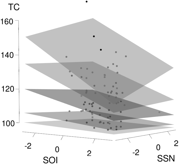
As illustrated in Figure 6, wind speed increases with decreasing SOI, which is expected as small SOI is associated with El Nino warming events, which in turn favour extreme cyclones, as explained in ?). As in ?), SSN is generally positive associated with extreme winds, but this is not a statistically significant association. From SOI parameter estimates’ plot, we can also see that PQR provides smoother and nicer estimates than freqQR, which lack borrowing strenght from the neighbours $\tau$. Due to the rigid non-crossing constraints, BSquare parameter estimates SOI and SSN are constant and lie mostly outside PQR $90\%$ confidence interval. GPQR produced generally smaller estimates than PQR and freqQR in the SOI parameter across the quantile levels. For the SSN parameter, GPQR produced smaller estimates only in the lower quantiles, while the other estimates largely agree with PQR and freqQR. Therefore, in the event that the data truly follow the GPD distribution, by placing priors centered on this distribution, we retain some advantages of using the parametric model for inference, and should perform better than models that cannot incorporate this information. However, in the case where data deviates from GPD, the pyramid quantile framework can correct for this misspecification with increasing data. So the ability of the pyramid quantiles to place informative priors allows us to fully take advantage of the Bayesian inferential framework.

Regression with large numbers of covariates poses additional computational challenges for the proposed method. Here we consider the University of Massachusetts Aids Research Unit IMPACT study data (UIS) available in the quantreg package in R, from ?), and analysed by ?), ?) and ?) using quantile regression. For this analysis with right censoring, the log-likelihood is now the sum over $i=1,\dots,n$ of

where $f(y_{i}|{\bf x}_{i})$ is given by Equation 7, where $F(y_{i}|{\bf x}_{i})$ is the corresponding CDF and where $c_{i}$ is the censoring status (1=right censored, 0=otherwise).

The dataset contains records for 575 observations, we estimated the conditional quantiles for the logarithm of the time to return to drug use ($Y$) as linear functions of 8 predictors, BECK (a depression score), FRAC (a compliance factor), AGE (age at enrollment), TREAT (current treatment assignment, 1= Long course, 0=Short course), NDT (number of previous drug treatment), RACE (1=Non-white, 0=White), IV3 (recent intravenous drug use, 1=Yes, 0=No), SITE (treatment site). All variables were scaled by subtracting their mean and dividing by their range. We fit the quantile levels $\tau=0.1,0.2,\ldots,0.9$ using 9 quantile pyramids and the Gaussian centring distribution, this amounts to a problem with 99 parameters. For high dimensions, the strategy described in Section 3.5 requires several modifications.

Firstly, existing off-the-shelf convex hull algorithms encounter memory problems for dimensions higher than 7 or 8. Here our strategy is to compute the convex hull of the data expressed in the space given by their leading 5 or 6 principal components, then to choose the remaining vertices by random sampling. We trial 500 random samples in this fashion, and select the pyramid locations that has the maximum distance between the quantile levels over the $P+1$ locations. Non-crossing constraint is then verified at all data points.

In higher dimensions, we also have noticed that well placed pyramid locations can greatly improve the MCMC mixing since the parameters are often highly correlated. For the current problem, we perform several parallel runs, each corresponding to a different set of pyramid locations, and choose the best mixing chain. More precisely for each chain we performed a trial MCMC run of 20.000 of standard MCMC, updating one parameter at a time, with tuning of proposal variance to obtain acceptance probability of roughly 0.44 for each parameter. This step allows us to learn the covariance structure of the parameters.

References

- Bondell et al. (2010 Bondell, H. D., B. J. Reich, and H. Wang (2010). Noncrossing quantile regression curve estimation. Biometrika 97(4), 825–838.
- Chernozhukov et al. (2009 Chernozhukov, V., I. Fernandez-Val, and A. Galichon (2009). Improving point and interval estimators of monotone functions by rearrangement. Biometrika 96, 559–575.
- Coles (2001 Coles, S. G. (2001). An introduction to statistical modeling of extreme values. Springer Verlag, London.
- Dette and Volgushev (2008 Dette, H. and S. Volgushev (2008). Non-crossing non-parametric estimates of quantile curves. Journal of Royal Statistical Society B 70, 609–627.
- Fang et al. (2015 Fang, Y., Y. Chen, and X. He (2015). Bayesian quantile regression with approximate likelihood. Bernoulli 21(2), 832–580.
- Ferguson (1974 Ferguson, T. S. (1974). Prior distributions on spaces of probability measures. Annals of Statistics 2, 615–629.
- Hall et al. (1999 Hall, P., R. C. L. Wolff, and Q. Yao (1999). Methods for estimating a conditional distribution function. Journal of American Statistical Association 94, 154– 163.
- Hanson and Johnson (2002 Hanson, T. and W. O. Johnson (2002). Modelling regression error with a mixture of Pólya trees. Journal of American Statistical Association 97(460), 1020–1033.
- He (1997 He, X. (1997). Quantile curves without crossing. American Statistician 51, 186–192.
- Hjort and Walker (2009 Hjort, N. L. and S. G. Walker (2009). Quantile pyramids for Bayesian nonparametrics. Annals of Statistics 37(1), 105–131.
- Hosmer and Lemeshow (1998 Hosmer, D. and S. Lemeshow (1998). Applied survival analysis: Regression modeling of time to event data. New Yori: John Wiley and Sons Inc.
- Jagger and Elsner (2009 Jagger, T. H. and J. B. Elsner (2009). Modeling tropical cyclone intensity with quantile regression. International Journal of Climatology 29, 1351–1361.
- Koenker (2005 Koenker, R. (2005). Quantile regression, Volume 38 of Econometric Society Monographs. Cambridge: Cambridge University Press.
- Koenker and Bassett (1978 Koenker, R. and J. Bassett, Gilbert (1978). Regression quantiles. Econometrica 46(1), 33–50.
- Kottas and Gelfand (2001 Kottas, A. and A. E. Gelfand (2001). Bayesian semiparametric median regression modelling. Journal of American Statistical Association 96, 1458–1468.
- Kottas and Krnjajić (2009 Kottas, A. and M. Krnjajić (2009). Bayesian semiparametric modelling in quantile regression. Scandinavian Journal of Statistics 36, 297–319.
- Lavine (1992 Lavine, M. (1992). Some aspects of Pólya tree distributions for statistical modelling. Annals of Statistics 20(3), 1222–1235.
- Lavine (1994 Lavine, M. (1994). More aspects of Pólya tree distributions for statistical modelling. Annals of Statistics 22, 1161–1176.
- Portnoy (2003 Portnoy, S. (2003). Censored quantile regression. Journal of American Statistical Association, 1001–1012.
- R Core Team (2014 R Core Team (2014). R: A Language and Environment for Statistical Computing. Vienna, Austria: R Foundation for Statistical Computing.
- Reich et al. (2008 Reich, B. J., H. D. Bondell, and H. J. Wang (2008). Flexible Bayesian quantile regression for independent and clustered data. Biostatistics 11, 337–352.
- Reich et al. (2011 Reich, B. J., M. Fuentes, and D. B. Dunson (2011). Bayesian spatial quantile regression. Journal of the American Statistical Association 106(493), 6–20.
- Reich and Smith (2013 Reich, B. J. and L. B. Smith (2013). Bayesian quantile regression for censored data. Biometrics 69, 651–660.
- Rodrigues and Fan (2016 Rodrigues, T. and Y. Fan (2016). Regression adjustment for noncrossing Bayesian quantile regression. Journal of Computational and Graphical Statistics. (in press).
- Smith and Reich (2013 Smith, L. and B. Reich (2013). BSquare: Bayesian Simultaneous Quantile Regression. R package version 1.1.
- Sriram et al. (2013 Sriram, K., R. V. Ramamoorthi, and P. Ghosh (2013). Posterior consistency of bayesian quantile regression based on the misspeficied asymmetric Laplace density. Bayesian Analysis 8(2), 1–26.
- Tokdar (2015 Tokdar, S. (2015). qrjoint: Joint Estimation in Linear Quantile Regression. R package version 0.1-1.
- Tokdar and Kadane (2012 Tokdar, S. T. and J. B. Kadane (2012). Simultaneous linear quantile regression: a semiparametric Bayesian approach. Bayesian Analysis 7(1), 51–72.
- Yang and Tokdar (2017 Yang, Y. and S. Tokdar (2017). Joint estimation of quantile planes over arbitrary predictor spaces. Journal of the American Statistical Association. (in press).
- Yu and Moyeed (2001 Yu, K. and R. A. Moyeed (2001). Bayesian quantile regression. Statist. Probab. Lett. 54(4), 437–447.
Appendix
For clarity we give the demonstrations for the case , the generalization to with within the convex hull of the pyramid locations being straightforward. For , without loss of generality, we suppose that and so that, for and any ,
where and are independent pyramid quantile processes.
We have and where and are independent pyramid quantile processes centered on the uniform distribution on .
We suppose that and are a.s. absolutely continuous and
we suppose that the two centring quantile functions and are also absolutely continuous.
Thus and are a.s. absolutely continuous and
we denote and the corresponding quantile density functions.
Then, for any , the conditional quantile function is also a.s. absolutely continuous with quantile density function .
Proof of Proposition 1
We first show that conditions similar to (B) and (C) are also true at any :
-
for all there exists an such that, ,
for any function from to for which .
We use the log sum inequality and see that, ,and by using condition (B) we get the result.
the density is bounded by some .
Under the condition (C) and are bounded by some finite and . Since we have, ,thus, ,
Once these properties are stated we can follow step by step the lines of the proof of Proposition 3.1 in ?). For any in , by using the change of variable , the Kullback-Leibler divergence between and can be decomposed as
where . Proceeding as in ?), and using conditions and , the first term in this sum is smaller than any arbitrary positive value with positive prior probability mass if, for any , the prior puts positive probability mass on where . To prove that this sufficient condition is true note that we have, ,
Now, from condition (A), the prior puts positive probability mass on and for any positive and . Thus, from the absolute continuity of and , the prior puts positive probability mass on and for any positive and and so, using the preceding inequality, puts positive probability mass on for any positive . By using the absolute continuity of we finally get that, for any positive , the prior puts positive probability mass on .
For the second term in the sum we use again the consequence of condition (A): the prior puts positive probability mass on for any positive then, using the absolute continuity of , puts positive probability mass on for any . Hence, using the property , this term is also bounded by any positive real with positive probability and finally we know that the prior put positive probability mass on .
To complete the proof note that this result is true for any and we have, for any ,
Since
we get the desired result.
Proof of Proposition 2
We have just to follow the steps of the proof of proposition 7.1 in ?) and to note that the Hellinger distance is given by
and that, if , , are the quantile sampled by , if for , if we have both and then, ,
It turns out that, for a given , , there exits such that if and then . Once this is stated the rest of the proof of ?) applies.