Adaptive Cross-Packet HARQ

Mohammed Jabi Abdellatif Benyouss Maël Le Treust Étienne Pierre-Doray Leszek Szczecinski ^†^†thanks: M. Jabi, A. Benyouss, and L. Szczecinski are with INRS-EMT, University of Quebec, Montreal, Canada. e-mail: {benyouss,jabi,leszek}@emt.inrs.ca, ^†^†thanks: E. Pierre-Doray is with Polytechnique de Montréal, Canada; he was also with INRS-EMT when this work was carried out. e-mail: {etipdoray@gmail.com} ^†^†thanks: M.˜Le Treust is with ETIS - UMR 8051 / ENSEA - Université de Cergy-Pontoise - CNRS, France. e-mail: {mael.le-treust@ensea.fr.}^†^†thanks: Part of this work was presented at the IEEE Wireless Commun. Network. Conf. (WCNC), Doha, Qatar, April 2016.

Abstract

In this work, we investigate a coding strategy devised to increase the throughput in hybrid ARQ (HARQ) transmission over block fading channel. In our approach, the transmitter jointly encodes a variable number of bits for each round of HARQ. The parameters (rates) of this joint coding can vary and may be based on the negative acknowledgment (NACK) provided by the receiver or, on the past (outdated) information about the channel states. These new degrees of freedom allow us to improve the match between the codebook and the channel states experienced by the receiver. The results indicate that significant gains can be obtained using the proposed coding strategy, particularly notable when the conventional HARQ fails to offer throughput improvement even if the number of transmission rounds is increased. The new cross-packet HARQ is also implemented using turbo codes where we show that the theoretically predicted throughput gains materialize in practice, and we discuss the implementation challenges.

I Introduction

In this work, in order to improve the throughput of the HARQ transmission over block-fading channel, we propose to use joint coding of multiple information packets into the same channel block and we develop methods to optimize the coding rates.

HARQ is used in modern communications systems to deal with unpredictable changes in the channel (due to fading), and with the distortion of the transmitted signals (due to noise). HARQ relies on the feedback/acknowledgement channel, which is used by the receiver to inform the transmitter about the decoding errors (via NACK) and about the decoding success, via positive acknowledgment (ACK). After NACK, the transmitter makes another transmission round which conveys additional information necessary to decode the packet. This continues till ACK is receiver and then a new HARQ cycle starts again for another information packet. In so-called truncated HARQ, the cycle stops also if the maximum number of rounds is attained.

As in many previous works, e.g., [1, 2], we will consider throughput as a performance measure assuming that residual errors are taken care of by the upper layers [3]. We consider here the “canonical” problem defined in [1], where the channel state information (CSI) is available at the receiver but not at the transmitter, which knows only its statistical description. The essential part of HARQ is channel coding, which is done over many channel blocks as long as NACK s are obtained over the feedback channel.

It was shown in [1] that HARQ’s throughput may approach the ergodic capacity of the channel with sufficiently high “nominal” coding rate per round. However, such an approach is based on large number of HARQ rounds, and thus has a limited practical value: long buffers are required which becomes a limiting factor for implementation of HARQ [4].

On the other hand, using finite nominal coding rate and truncated HARQ, the difference between the throughput achievable using HARQ and the theoretical limits may be large, especially, when we target throughput close to the nominal rate [2], [5].

To address this problem, various adaptive versions of HARQ were proposed in the literature. For example, [6, 7, 8, 9, 10, 11, 12] suggested to vary the length of the codewords so as to strike the balance between the number of channel uses and the chances of successful decoding. Their obvious drawback is that the resources assigned to the various HARQ rounds are not constant which may leave an “empty” space within the block.

To deal with this issue, it was proposed to share the block resources (power, time or bandwidth) between various packets in e.g., [13, 14, 15, 16, 3], to encode many packets into predefined size blocks as done in [17, 18], or to group variable-length codewords to fill the channel block [19, 11]. A simplified approach was also proposed in [20] to transmit the redundancy using two-step encoding.

These approaches implicitly implement a joint coding of many packets into a single channel block. Here, we want to address the issue of cross-packet coding explicitly. The idea of this Cross-packet HARQ (XP-HARQ) is to get rid of the restricting assumptions proper to various heuristics developed before and to use a generic joint HARQ encoder accepting many information packets and encoding them into a common codeword which fills the channel block.

The contributions of this work are the following:

•

We propose a general framework to analyze joint encoding of multiple packets which allow us to derive the relationship between the coding rates and the throughput. Our approach to cross-packet coding is similar to the one shown in [21, 22, 23, 24], which, however, did not optimize the coding parameters. The optimization was proposed in [25], however, due to complex decoding rules, it was very tedious and thus limited to the case of a simple channel model. In our work we simplify the problem assuming asymptotically long codewords are used, which leads to a compact description of the decoding criteria and allows us to solve the rate-optimization problem.
•

We consider the so-called multi-bit feedback to adapt the coding rates to the channel state experienced by the receiver in the past transmission rounds of HARQ. The same idea was exploited already e.g., in[26, 27, 11, 6, 28, 29, 9, 30, 31, 12, 3]. The assumption of multi-bit feedback not only simplifies the optimization but also yields the results which may be treated as the ultimate performance limits of any adaptation schemes when the instantaneous CSI is not available at the transmitter.
•

We optimize the coding rates using the Markov decision process (MDP) formulation [32, Chap. 4], and compare the proposed, XP-HARQ to the conventional incremental redundancy HARQ (IR-HARQ) from the perspective of attainable throughput. For the particular case of two transmission round, we obtain the optimal solution in closed-form.
•

We also present an analytical formula for attainable throughput using heuristic rate-adaptation inspired by the numerical results and which presents a notable gain over the conventional IR-HARQ.
•

To obtain an insight into the practical constraints on the system design, we also show the results obtained when a turbo coding is adopted.

The remainder of the paper is organized as follows. We define the transmission model as well as the basic performance metrics in Sec. II. The idea of cross-packet coding is explained in Sec. III. The optimization of the rates in the proposed coding strategy is presented in Sec. IV. We discuss the effects of using a practical encoding/decoding schemes in Sec. V. The numerical results are presented in form of short examples throughout the work to illustrate the main ideas. Conclusions are presented in Sec. VI. The optimization methods used to obtain the numerical results and the proof of decoding conditions are presented in appendices.

II Channel model and HARQ

We consider a point-to-point IR-HARQ transmission of a packet $\mathsf{m}$ over a block fading channel. After each transmission, using a feedback/acknowledgement channel, the receiver tells the transmitter whether the decoding of $\mathsf{m}$ succeeded (ACK) or failed (NACK). We thus assume that error detection is possible (e.g., via cyclic redundancy check (CRC) mechanisms) and that the feedback channel is error-free. For simplicity, we ignore any loss of resources due to the CRC and the acknowledgement feedback.

The transmission of a single packet may thus require many transmission rounds which continue till the $K$ th round is reached or till ACK is received. When $K$ is finite, we say that HARQ is truncated, otherwise we say it is persistent. We define a HARQ cycle as the sequence of transmission rounds of the same packet $\mathsf{m}$ .

The received signal in the $k$ th round is given by

\displaystyle\boldsymbol{y}_{k}=\sqrt{\mathsf{snr}_{k}}\boldsymbol{x}_{k}+\boldsymbol{z}_{k},\quad k=1,\ldots,K

(1)

where $\boldsymbol{z}_{k}$ and $\boldsymbol{x}_{k}$ modelling, respectively, the noise and the transmitted codeword are ${\mathop{N_{\textnormal{s}}}}$ -dimensional vectors, each containing independent, identically distributed (i.i.d.) zero mean, unit-variance random variables; $\mathsf{snr}_{k}$ is thus the signal-to-noise ratio (SNR) at the receiver. The elements of $\boldsymbol{z}_{k}$ are drawn from complex Gaussian distribution, and elements of $\boldsymbol{x}_{k}$ – from the uniform distribution over the set (constellation) $\mathcal{X}$ .

During the $k$ th round, $\mathsf{snr}_{k}$ is assumed to be perfectly known/estimated at the receiver and unknown at the transmitter; it varies from one round to another and we model $\mathsf{snr}_{k},k=1,\ldots,K$ as the i.i.d. random variables $\mathsf{SNR}$ with distribution $p_{\mathsf{SNR}}(\mathsf{snr})$ .

II-A Conventional HARQ

In the conventional IR-HARQ, a packet $\mathsf{m}\in\{0,1\}^{R{\mathop{N_{\textnormal{s}}}}}$ is firstly encoded into a codeword $\boldsymbol{x}=\Phi[\mathsf{m}]\in\mathcal{X}^{K{\mathop{N_{\textnormal{s}}}}}$ composed of $K{\mathop{N_{\textnormal{s}}}}$ complex symbols taken from a constellation $\mathcal{X}$ where $\Phi[\cdot]$ is the coding function and $R$ denotes the nominal coding rate per block.¹¹ 1 We clearly define the nominal rate as the coding rate per channel block because HARQ is a variable-rate transmission: the number of used channel blocks is random, and the final transmission rate is random as well. Then, the codeword $\boldsymbol{x}$ is divided into $K$ disjoint subcodewords $\boldsymbol{x}_{k}$ composed of different symbols i.e., $\boldsymbol{x}=[\boldsymbol{x}_{1},\boldsymbol{x}_{2},\ldots,\boldsymbol{x}_{K}]$ . After each round $k$ , the receiver try to decode the packet $\mathsf{m}$ concatenating all received channel outcomes till the $k$ th block

\displaystyle\boldsymbol{y}_{[k]}=[\boldsymbol{y}_{1},\ldots,\boldsymbol{y}_{k-1},\boldsymbol{y}_{k}].

(2)

Following [1, 27], we assume ${\mathop{N_{\textnormal{s}}}}$ large enough to make the random coding limits valid. Then, knowing the mutual information (MI) $I_{k}=\mathsf{I}(X_{k};Y_{k}|\mathsf{snr}_{k})$ between the random variables $X_{k}$ and $Y_{k}$ modeling respectively, the channel input and output in the $k$ th block, allows us to determine when the decoding is successful or not: the decoding failure occurs in the $k$ th round if the accumulated MI at the receiver is smaller than the coding rate

	$\displaystyle\mathsf{NACK}_{k}$	$\displaystyle\triangleq\{\big(I_{1}<R\big)\wedge\big(I^{\Sigma}_{2}<R\big)\wedge\ldots\wedge\big(I^{\Sigma}_{k}<R\big)\}$		(3)
		$\displaystyle=\left\{I^{\Sigma}_{k}<R\right\},$		(4)

where $I^{\Sigma}_{k}\triangleq\sum_{l=1}^{k}I_{l}$ is the MI accumulated in $k$ rounds. Of course, the MI depends on the SNR, i.e., $I_{k}\equiv I_{k}(\mathsf{snr}_{k})$ .

IR-HARQ can be modelled as a Markov chain where the transmission rounds correspond to the states, and the HARQ cycle corresponds to a renewal cycle in the chain. Thus, the long-term average throughput, defined as the average number of correctly received bits per transmitted symbol, may be calculated from the renewal-reward theorem: it is a ratio between the average reward (number of bits successfully decoded per cycle) and the average renewal time (the expected number of transmissions needed to deliver the packet with up to $K$ transmission rounds) [1].

Let $f_{k}\triangleq\Pr\left\{\mathsf{NACK}_{k}\right\},k\geq 1$ be the probability of $k$ successive errors so the probability of successful decoding in the $k$ th round is given by $\Pr\left\{\mathsf{NACK}_{k-1}\wedge I^{\Sigma}_{k}\geq R\right\}=f_{k-1}-f_{k}$ [1]. The throughput is then calculated as follows [1]

	$\displaystyle\eta^{{\textnormal{ir}}}_{K}$	$\displaystyle=\frac{R(1-f_{1})+R(f_{1}-f_{2})+\ldots+R(f_{K-1}-f_{K})}{1\cdot(1-f_{1})+2\cdot(f_{1}-f_{2})+\ldots+K\cdot(f_{K-1})}$		(5)
		$\displaystyle=\frac{R(1-f_{K})}{1+\sum_{k=1}^{K-1}f_{k}}.$		(6)

Because the instantaneous CSI is not available at the transmitter, the highest achievable throughput is given by the ergodic capacity²² 2 We use the term “capacity” to denote the achievable rate for a given distribution of $X$ . of the channel [1, 33]

\displaystyle\overline{C}\triangleq\mathds{E}_{\mathsf{SNR}}[I(\mathsf{SNR}]).

(7)

However, achieving $\overline{C}$ is not obvious: as shown in [1], it can be done growing simultaneously $R$ and $K$ to infinity but this approach is impractical due to large memory requirements.

Example 1 (Two-states channel).

Consider a block-fading channel where the MI can only take two values, $I_{\textnormal{a}}$ and $I_{\textnormal{b}}$ , where $\Pr\left\{I=I_{\textnormal{a}}\right\}=1-p$ and $\Pr\left\{I=I_{\textnormal{b}}\right\}=p$ . The ergodic capacity is given by $\overline{C}=I_{\textnormal{a}}(1-p)+I_{\textnormal{b}}p$ . We force the HARQ to deliver the packet at most in the last transmission, i.e., $f_{K}=0$ , which means that we impose the constraints on the coding rate $R\leq KI_{\textnormal{a}}$ if we assume that $I_{\textnormal{a}}<I_{\textnormal{b}}$ .

Assume $I_{\textnormal{a}}=1,I_{\textnormal{b}}=1.5$ , and $p=0.75$ so $\overline{C}=1.375$ . For $K=2,3$ we easily calculate the throughput³³ 3 For $R\leq 1$ we obtain $f_{1}=0$ . For $1<R\leq 1.5$ – $f_{1}=1-p$ and $f_{2}=0$ . For $1.5<R\leq 2$ – $f_{1}=1$ , $f_{2}=0$ , etc. as

\displaystyle\eta^{{\textnormal{ir}}}_{2}

\displaystyle=\begin{cases}R,&\text{if}\quad R\leq 1\\ 0.8R,&\text{if}\quad 1<R\leq 1.5\\ 0.5R,&\text{if}\quad 1.5<R\leq 2\end{cases},

(8)

and

\displaystyle\eta^{{\textnormal{ir}}}_{3}

\displaystyle=\begin{cases}\eta^{{\textnormal{ir}}}_{2},&\text{if}\quad R\leq 2\\ 0.48R,&\text{if}\quad 2<R\leq 2.5\\ 0.41R,&\text{if}\quad 2.5<R\leq 3\end{cases}.

(9)

The optimum throughput-rate pairs are then $(\eta^{{\textnormal{ir}}}_{2}=1.2,R=1.5)$ and $(\eta^{{\textnormal{ir}}}_{3}=1.23,R=3)$ . First, the benefit of using HARQ is clear: we are able to transmit without errors with a finite number of channel blocks and go beyond the obvious limit of $I_{\textnormal{a}}$ . Second, we note that for $K=2$ , after two transmissions, the accumulated MI always satisfies $I^{\Sigma}_{2}\geq 2$ , while the condition $I^{\Sigma}_{2}\geq 1.5$ is sufficient to decode the packet. This may be seen as a “waste” which will be removed with the idea of cross-packet coding introduced in Sec. III.

Example 2 (16QAM over Rayleigh fading channel).

Assume now that the transmission is done using symbols drawn uniformly from 16-points quadrature amplitude modulation (QAM) constellation $\mathcal{X}$ [34, Ch. 2.5] and that the channel gains follow Rayleigh distribution, i.e.,

\displaystyle p_{\mathsf{SNR}}(\mathsf{snr})=1/\overline{\mathsf{snr}}\exp(-\mathsf{snr}/\overline{\mathsf{snr}}),

(10)

where $\overline{\mathsf{snr}}$ is the average SNR.

We calculate $I(\mathsf{snr})$ and the average $\overline{C}$ using the numerical methods outlined in [34, Ch. 4.5] and compare it in Fig. 1 with the throughput $\eta^{{\textnormal{ir}}}_{K}$ when $K\in\{2,\infty\}$ .⁴⁴ 4 $\eta^{{\textnormal{ir}}}_{\infty}$ can be computed by taking $K$ large enough in (5) as suggested in [2] or by evaluating the throughput using the method outlined in the Appendix B and considering the policy $\pi(\mathsf{s})=R$ if $\mathsf{s}=(0,0)$ and $\pi(\mathsf{s})=0$ otherwise. We opt for the later method. The results indicate that i) there is a significant loss with respect to the ergodic capacity when using truncated HARQ, and ii) increasing the number of transmission rounds ( $K=\infty$ ) helps recovering the loss for a small-medium range of throughput (e.g., for $\eta^{{\textnormal{ir}}}=1$ we gain $\sim 3{\textnormal{dB}}$ and the gap to $\overline{C}$ is less than $1{\textnormal{dB}}$ ), but it is less useful in the region of high $\eta^{{\textnormal{ir}}}_{K}$ , i.e., in the vicinity of the maximum attainable throughput (e.g., for $\eta^{{\textnormal{ir}}}=3$ , we gain $1{\textnormal{dB}}$ but the gap to $\overline{C}$ is still $\sim 5{\textnormal{dB}}$ ). We highlight this well-known effect [2] to emphasize later the gains of the new coding strategy.

Fig. 1: Throughput of the conventional IR-HARQ, compared to the ergodic capacity,

\overline{C}

, in Rayleigh block-fading channel. The

R_{\textrm{opt}}

curve is an envelope of the throughputs

\eta^{{\textnormal{ir}}}_{K}

obtained with different coding rates per block

R\in\{0.25,0.5,\ldots,7.75\}

III Cross-packet HARQ

The examples shown previously indicate that the conventional coding cannot bring the throughput of HARQ close to the capacity unless the nominal coding rate $R$ and the number of rounds $K$ increase. We would like now to exploit a new coding possibility consisting in joint coding of packets during the HARQ cycle.

Let us start with the case of two transmission rounds. In the first round, we use the nominal rate $R_{1}$ is used, i.e., the packet $\mathsf{m}_{1}\in\{0,1\}^{R_{1}{\mathop{N_{\textnormal{s}}}}}$ is encoded

\displaystyle\boldsymbol{x}_{1}=\Phi_{1}[\mathsf{m}_{1}]\in\mathcal{X}^{{\mathop{N_{\textnormal{s}}}}},

(11)

and transmitted over the channel (1) producing $\boldsymbol{y}_{1}=\sqrt{\mathsf{snr}_{1}}\boldsymbol{x}_{1}+\boldsymbol{z}_{1}$ , where $\Phi_{k}[\cdot]$ is the encoding at the $k$ th round.

If the packet $\mathsf{m}_{1}$ is decoded correctly (which occurs if $I_{1}\geq R_{1}$ ), a new cycle HARQ starts by the transmission of a new packet. However, if the decoding fails, the packet $\mathsf{m}_{[2]}=[\mathsf{m}_{1},\mathsf{m}_{2}]\in\mathbb{B}^{(R_{1}+R_{2}){\mathop{N_{\textnormal{s}}}}}$ is encoded using a conventional code designed independently of the codebook corresponding to the first transmission

\displaystyle\boldsymbol{x}_{2}=\Phi_{2}[\mathsf{m}_{1},\mathsf{m}_{2}]\in\mathcal{X}^{{\mathop{N_{\textnormal{s}}}}},

(12)

which yields the channel outcome $\boldsymbol{y}_{2}=\sqrt{\mathsf{snr}_{2}}\boldsymbol{x}_{2}+\boldsymbol{z}_{2}$ as depicted in Fig. 2.⁵⁵ 5 This coding strategy is introduced without any claim of optimality. The undeniable advantage of using independently generated codebooks is the simplicity of implementation. We note that the idea of using $\Phi_{2}$ independent of $\Phi_{1}$ was also proposed in [24, 25].

Fig. 2: Model of the adaptive XP-HARQ transmission: the HARQ controller uses the information

\mathcal{F}

obtained over the feedback channel to choose the rate for the next round;

\mathcal{F}

represent ACK/NACK acknowledgement in the case of one bit feedback, or, it carries the index of the coding rate in the case of rate-adaptive transmission (Sec. IV-A).

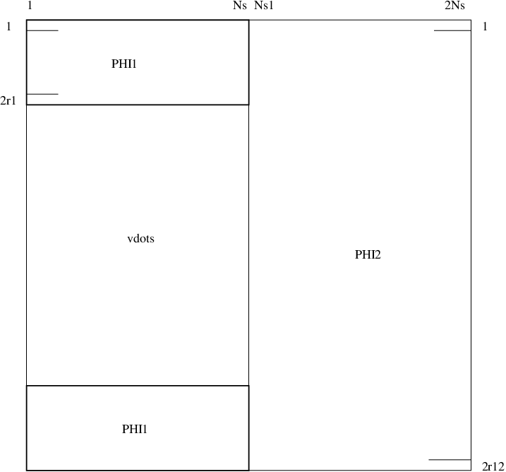
Intuitively, by introducing $\mathsf{m}_{2}$ we want to prevent the “waste” of MI, which happens if $I^{\Sigma}_{2}$ is much larger than $R_{1}$ , cf. Example 1. After the second transmission, the receiver decodes the packets $[\mathsf{m}_{1},\mathsf{m}_{2}]$ using the observations $\boldsymbol{y}_{[2]}=[\boldsymbol{y}_{1},\boldsymbol{y}_{2}]$ . The codebook obtained after two transmissions is illustrated in Fig. 3. The associated decoding conditions based on the channel outcomes $\boldsymbol{y}_{[2]}$ are given by

	$\displaystyle I^{\Sigma}_{2}=I_{1}+I_{2}$	$\displaystyle\geq R_{1}+R_{2},$		(13)
	$\displaystyle I_{2}$	$\displaystyle\geq R_{2},$		(14)

where (13) is a constraint over the sum-rate that guarantees the joint decoding of the packets pair $(\mathsf{m}_{1},\mathsf{m}_{2})$ while (14) ensures the correct decoding of the packet $\mathsf{m}_{2}$ . This means, the MI must be accumulated to decode each of the packets even though the decoding is done jointly. The formal proof of (13) and (14) is presented in the Appendix A. Similar decoding conditions were presented in the context of physical layer (PHY) security in [35].

While the event $\mathsf{NACK}_{1}$ remains unchanged with respect to the conventional coding, the event $\mathsf{NACK}_{2}$ means that $\mathsf{NACK}_{1}$ occurred, as well as, that (13) and (14) are not satisfied

$\displaystyle\mathsf{NACK}_{2}$	$\displaystyle=\Big\{\bigl(I_{1}<R_{1}\bigr)\wedge\overline{\bigl((I^{\Sigma}_{2}\geq R^{\Sigma}_{2})\wedge(I_{2}\geq R_{2})\bigr)}\Big\}$
	$\displaystyle=\Big\{(I_{1}<R_{1})\wedge\bigl((I^{\Sigma}_{2}<R^{\Sigma}_{2})\vee(I_{2}<R_{2})\bigr)\Big\}$	(15)
	$\displaystyle=\Big\{\bigl(I_{1}<R_{1}\bigr)\wedge\bigl(I^{\Sigma}_{2}<R^{\Sigma}_{2}\bigr)\Big\},$	(16)

where $R^{\Sigma}_{k}\triangleq\sum_{l=1}^{k}R_{l}$ and the event $\overline{E}$ is the complement of $E$ . To pass from (15) to (16) we used the decoding failure implication

\displaystyle\{I_{1}<R_{1}\wedge I_{2}<R_{2}\}\implies\{I_{1}<R_{1}\wedge I^{\Sigma}_{2}<R^{\Sigma}_{2}\},

which means that $\mathsf{NACK}_{1}$ combined with (13) implies (14).

The above conditions generalize straightforwardly for any $k>1$ with $R_{k}$ being the rate of the packet $\mathsf{m}_{k}$ added in the $k$ th round

\displaystyle\mathsf{NACK}_{k}=\{\mathsf{NACK}_{k-1}\wedge\bigl(I^{\Sigma}_{k}<R^{\Sigma}_{k}\bigr)\}.

(17)

To calculate the throughput of such an XP-HARQ, we adopt a similar approach as in (5) but we must account for the reward in the $k$ transmission round given by $R^{\Sigma}_{k}$ , which yields

	$\displaystyle\eta^{{\textnormal{xp}}}_{K}$	$\displaystyle=\frac{R^{\Sigma}_{1}(1-f_{1})+R^{\Sigma}_{2}(f_{1}-f_{2})+\ldots+R^{\Sigma}_{K}(f_{K-1}-f_{K})}{(1-f_{1})+2\cdot(f_{1}-f_{2})+\ldots+K\cdot(f_{K-1})}$
		$\displaystyle=\frac{\sum_{k=1}^{K}R_{k}\big(f_{k-1}-f_{K}\big)}{1+\sum_{k=1}^{K-1}f_{k}}.$		(18)

Here, again $f_{k}=\Pr\left\{\mathsf{NACK}_{k}\right\},k\geq 1$ with $\mathsf{NACK}_{k}$ defined by (17).

As a sanity check we can set $R_{k}=0,k=2,\ldots,K$ , and recover the conventional single-packet HARQ, i.e., (18) will be equivalent to (6).

The fundamental difference of the proposed XP-HARQ with respect to the conventional HARQ appears now clearly in the numerator of (18) which expresses the idea of variable rate transmission due to encoding of multiple packets. Nevertheless, not only the numerator changed with respect to (6) but also the denominator is different due to the new definition of $\mathsf{NACK}_{k}$ in (17).

Refer to caption — Fig. 3: Illustration of the codebook defined through the coding function $\Phi_{1}$ in (11) and the joint coding function $\Phi_{2}$ in (12). Each codeword composed of $2{\mathop{N_{\textnormal{s}}}}$ symbols is indexed by the packet $\mathsf{m}_{[2]}$ . The first ${\mathop{N_{\textnormal{s}}}}$ symbols are created without indexing by $\mathsf{m}_{2}$ so we artificially repeat them $2^{R_{2}{\mathop{N_{\textnormal{s}}}}}$ times to match the number of codewords in the codebook $\Phi_{2}$ .

Example 3 (Two-state channel and XP-HARQ).

We consider now the proposed XP-HARQ in the scenario of Example 1. Let us start, as before, with $K=2$ and $R_{1}=1.5$ . After a decoding failure (which means that we obtained $I_{1}=I_{\textnormal{a}}=1$ ), we are free to define any rate $R_{2}$ . In the absence of any formal criterion (more on that in Sec. IV), we take the following auxiliary (and somewhat ad-hoc) condition: we want to guarantee a non-zero successful decoding probability, i.e., $f_{2}<1$ . Here, since $I^{\Sigma}_{2}\in(2,2.5)$ , any $R_{2}\leq 1$ can ensure that $f_{2}<1$ . In particular, if the rate $R_{2}\leq 0.5$ we guarantee a much stronger condition $f_{2}=0$ .

For the case when $K=2$ and using $R_{2}=0.5$ , we obtain $f_{1}=0.25$ and $f_{2}=0$ . The throughput is then given by

\displaystyle\eta^{{\textnormal{xp}}}_{2}=\frac{R_{1}+0.25R_{2}}{1+0.25}=1.3.

(19)

Thus, we used exactly the same channel resources as in the conventional HARQ, obtained the same guarantee of successful decoding ( $f_{2}=0$ ) after two transmission rounds, but the throughput is larger.

The difference is that, while we still have $I^{\Sigma}_{2}\in(2,2.5)$ , we now use $R^{\Sigma}_{2}=2$ to eliminated the “waste” of MI in the conventional IR-HARQ, where $R^{\Sigma}_{2}=1.5$ . The improvement may be seen as the increase in the throughput (from $\eta^{{\textnormal{ir}}}_{2}=1.2$ to $\eta^{{\textnormal{xp}}}_{2}=1.3$ ) or as the reduction in the memory requirements (i.e., we obtain a better throughput with smaller $K$ , see $\eta^{{\textnormal{ir}}}_{3}=1.23$ in Example 1). The price to pay for this advantages is the possible increase in complexity of cross-packet encoding/decoding.

Similarly, for $K=3$ , we can use the larger value of $R_{2}$ (that guarantees our objective of decodability, $f_{2}<1$ ), i.e., $R_{2}=1$ . In this case, $f_{1}=0.25$ , and $f_{2}=\Pr\left\{I_{1}<1.5\wedge I^{\Sigma}_{2}<2.5\right\}=0.0625$ . In the third transmission we observe $I^{\Sigma}_{3}\in(3,3.5)$ so, using $R_{3}=0.5$ , we obtain $f_{3}=0$ and thus the throughput is calculated as

\displaystyle\eta_{3}^{{\textnormal{xp}}}=\frac{R_{1}+0.25R_{2}+0.0625R_{3}}{1+0.25+0.0625}\approx 1.36,

(20)

which is already quite close to $\overline{C}=1.375$ .

The improvement of the throughput in XP-HARQ is due to the way the codebook is constructed. While the conventional IR-HARQ, see Sec. II-A, makes a rigid separation of the codewords into the fixed-content subcodewords – an approach which is blind to the channel realizations, in XP-HARQ we match the information content of the codebook following the outcome of the transmissions.

IV Optimization of the coding rates

Our goal now is to evaluate how well the XP-HARQ can perform. To this end, we will have to find the optimal coding rates $R_{1},R_{2},\ldots,R_{K}$ which maximize throughput (18).

Since the objective function is highly non linear, we will use the exhaustive search: for a truncated HARQ this can be done with a manageable complexity.

Example 4 (16QAM, Rayleigh fading – continued).

In Fig. 4 we show the results of the exhaustive-search optimization of ${\eta}^{{\textnormal{xp}}}_{K}$ with ${\eta}^{{\textnormal{ir}}}_{K}$ ; for implementability, we limited the search space: IR-HARQ uses $R_{1}\in\{0,0.25,\ldots,3.75\}$ and XP-HARQ uses rates which satisfy $R^{\Sigma}_{K}\leq R_{\max}$ , with $R_{\max}=8$ ; $R_{1}\in\{0.25,\ldots,3.75\}$ , $R_{k}\in\{0,0.25,\ldots,3.75\}~\forall k\in\{2,\ldots,K\}$ .

We used here an additional constraints requires each transmission to have non zero probability of being decodable, that is $R_{k}<\log_{2}M,\forall k=1,\ldots,K$ , where $M=16$ . In fact, these constraints were always satisfied in XP-HARQ so they only affect IR-HARQ; we will relax them in the next example.

In terms of SNR required to attain $\eta=3$ , the gain of XP-HARQ over IR-HARQ varies from $1.5{\textnormal{dB}}$ (for $K=2$ ) to $2.5{\textnormal{dB}}$ (for $K=3$ ).

Fig. 4: Throughput of the conventional IR-HARQ (

\eta^{{\textnormal{ir}}}_{K}

) compared to XP-HARQ (

\eta^{{\textnormal{xp}}}_{K}

) in Rayleigh block-fading channel. The ergodic capacity (

\overline{C}

) is shown for reference.

IV-A Rate adaptation

The possibility of varying the rates during the HARQ cycle opens new optimization space and we want to explore it fully following the idea of adapting the transmission parameters in HARQ on the basis of obsolete CSI considered before, e.g., in [6, 8, 9, 36, 10, 11, 29].

The idea is to adapt the coding rates using obsolete CSI s, $I_{1},I_{2},\ldots,I_{k-1}$ ; this concept remains compatible with the assumption of transmitter operating without CSI knowledge because the obsolete CSI s $I_{1},I_{2},\ldots,I_{k-1}$ cannot be used in the $k$ th round to infer anything about $I_{k}$ (due to i.i.d. model of the SNR s).

Using this approach, the rate $R_{k}$ will not only depend on the MI s $I_{1},\ldots,I_{k-1}$ but also – on the past rates $R_{1},\ldots,R_{k}$ .⁶⁶ 6 Through $R_{1},R^{\Sigma}_{2},\ldots,R^{\Sigma}_{k-1}$ , which determine the probability of the decoding success, see (17). This recursive dependence may be dealt with using the MDP framework, where the states of the Markov chain not only indicate the transmission number but also gather all information necessary to decide on the rate, which in the language of the MDP is called an action. The state has to be defined so that i) knowing the action (chosen rate), the state-transition probability can be determined after each transmission, and ii) the reward may be calculated knowing the state and the action. The state defined as a pair $\mathsf{s}_{k}=(R^{\Sigma}_{k},I^{\Sigma}_{k})$ satisfies these two requirements, where we only need to consider the pairs which satisfy $R^{\Sigma}_{k}>I^{\Sigma}_{k}$ , otherwise the decoding is successful and the HARQ cycle terminates.

Thus, the rate adaptation consists in finding the functions (called policies), $R_{l}(\mathsf{s}_{l-1})$ maximizing the throughput, which is found generalizing the expression (18)

\displaystyle\hat{\eta}^{{\textnormal{xp}}}_{K}

\displaystyle=\frac{\mathds{E}\big[\sum_{k=1}^{K}\xi_{k}R^{\Sigma}_{k}\big]}{1+\sum_{k=1}^{K-1}f_{k}},

(21)

where

\displaystyle\xi_{k}=\mathds{I}\big[{I_{1}<R_{1}\wedge\ldots\wedge I^{\Sigma}_{k-1}<R^{\Sigma}_{k-1}\wedge I^{\Sigma}_{k}\geq R^{\Sigma}_{k}}\big],

(22)

indicates the successful decoding in the $k$ th round, and

\displaystyle R^{\Sigma}_{k}=R^{\Sigma}_{k-1}+R_{k}(\mathsf{s}_{k-1})

(23)

is the accumulated rate depending in a recursive fashion on the states of the Markov chain. The probability of $k$ successive errors, $f_{k}$ , may be expressed as (17) considering the dependence of the rates on the states given by (23). All the expectations are taken with respect to the states – or equivalently – with respect to $I_{1},\ldots,I_{K}$ .

The expression (21) will be useful in Sec. IV-B, however, its maximization with respect to the policies $R_{l}(\mathsf{s}_{l-1}),l=1,\ldots,K$ will be done using efficient specialized algorithms as explained in Appendix B. In the particular case of two HARQ rounds ( $K=2$ ), the optimal rate adaptation policy can be derived in closed form as shown in Appendix C.

To run the optimization algorithms outlined in Appendix B, we need to discretize the variables involved (states and actions). As for the rates (actions), we use a relatively course discretization step equal to $0.25$ and define the action space as the set $\mathcal{R}=\{0.25,0.5,\ldots,R_{\max}\}$ . While the results are notably affected by $R_{\max}$ , using a finer discretization step did not change the results significantly.

Here, it is natural to ask a question about the signaling overhead due to proposed adaptation scheme. We thus note that while we assume the outdated MI, $I^{\Sigma}_{k}$ is discretized with a high resolution when optimizing the throughput (cf. Appendix B), the feedback load is affected by the cardinality of the action space, $\mathcal{R}$ : the receiver knows the accumulated MI but only transmits the index of the chosen rate.

Example 5 (16QAM, Rayleigh fading channel – continued).

The throughput of adaptive XP-HARQ, $\hat{\eta}^{{\textnormal{xp}}}$ , is compared to the throughput of the conventional IR-HARQ in Fig. 5 for $K=\infty$ , while Fig. 6 shows the comparison for truncated HARQ.

Here, for IR-HARQ, we removed the constraints on the initial coding rate, $R_{1}<\log_{2}M$ , which were applied in Example 4. It allows us to increase the throughput $\eta^{{\textnormal{ir}}}_{3}$ at the cost of first transmission not being decodable. In our view this is a potentially serious drawback but we show such results to complement those already shown in Fig. 4, where the decodability condition was imposed. Again, XP-HARQ was insensitive to the decodability constraints and always provided results with decodable transmissions.

Fig. 5: Optimal throughput of the conventional IR-HARQ (

\eta^{{\textnormal{ir}}}_{\infty}

) compared to the proposed XP-HARQ (

\hat{\eta}^{{\textnormal{xp}}}_{\infty}

) in Rayleigh block-fading channel. The ergodic capacity (

\overline{C}

) is shown for reference.

Fig. 6: Throughput of the conventional IR-HARQ (

\eta^{{\textnormal{ir}}}_{K}

) compared to the proposed XP-HARQ (

\hat{\eta}^{{\textnormal{xp}}}_{K}

) for a truncated HARQ,

K\in\{2,3\}

in Rayleigh block-fading channel;

R_{\max}=8

. The ergodic capacity (

\overline{C}

) and the optimal throughput of the persistent conventional IR-HARQ (

\eta^{{\textnormal{ir}}}_{\infty}

) are shown for reference.

The improvements due to adaptive XP-HARQ are most notable for high values of the throughput. In particular we observe that

•

The persistent XP-HARQ halves the gap between the ergodic capacity and the conventional IR-HARQ. For example, the SNR gap between $\hat{\eta}^{{\textnormal{xp}}}_{\infty}=3$ and the ergodic capacity, $\overline{C}=3$ is reduced by more than $50\%$ when comparing to the gap between $\eta^{{\textnormal{ir}}}_{\infty}=3$ and $\overline{C}=3$ which is equal to $5{\textnormal{dB}}$ when $R_{\max}=8$ . We note that the throughput of XP-HARQ increases when $R_{\max}$ increases: the SNR gap between $\overline{C}$ and $\hat{\eta}^{{\textnormal{xp}}}_{\infty}$ is reduced by half when $R_{\max}=16$ is used instead of $R_{\max}=8$ .
•

For any value of throughput $\eta>3$ , two rounds of XP-HARQ yield higher throughput than the conventional persistent IR-HARQ. Thus, in this operation range we may improve the performance and yet decrease the memory requirements at the receiver.

IV-B Heuristic adaptation policy

Fig. 7: Optimal rate

R_{k}

as a function of

R^{\Sigma}_{k-1}-I^{\Sigma}_{k-1}

for different values of

R^{\Sigma}_{k-1}

;

K=\infty

\overline{\mathsf{snr}}=20{\textnormal{dB}}

R_{\max}=8

Fig. 7 shows the optimal rate adaptation as a function of $R^{\Sigma}_{k-1}-I^{\Sigma}_{k-1}$ for different values of $R^{\Sigma}_{k-1}$ , where we note a quasi-linear behaviour of the adaptation function with the saturation which occurs to guarantee $R^{\Sigma}_{k-1}+R_{k}\leq R_{\max}$ .

To exploit this very regular form, which was also observed solving the related problems in [11, 29], we propose to use the following heuristic function inspired by Fig. 7

\displaystyle R_{k}=R_{1}-(R^{\Sigma}_{k-1}-I^{\Sigma}_{k-1}),

(24)

where only the rate $R_{1}$ needs to be optimized (from Fig. 7 we find $R_{1}\approx 3.5$ ). Furthermore, applying (24) recursively we obtain $R_{2}=I_{1},R_{3}=I_{2},\ldots,R_{k}=I_{k-1}$ ; the identical rate-adaptation strategy may be derived from [20, Sec. III].

The simplicity of the adaptation function allows us now to evaluate analytically the throughput of XP-HARQ. To this end we need to calculate $f_{l}$ in the denominator of (21) and the expectation in its numerator.

We first note that, from (24) we obtain

\displaystyle\big(I^{\Sigma}_{k}

\displaystyle<R^{\Sigma}_{k}\big)\iff(I_{k}<R_{1}),

(25)

which means that the probability of decoding failure does not change with the index of the transmission round. Thus

\displaystyle f_{k}

\displaystyle=(f_{1})^{k},

(26)

and (22) may be formulated as

\displaystyle\xi_{k}=\Big(\prod_{l=1}^{k-1}\mathds{I}\big[{I_{l}<R_{1}}\big]\Big)\mathds{I}\big[{I_{k}\geq R_{1}}\big].

(27)

From (24) we also obtain $R^{\Sigma}_{k}=R_{1}+\sum_{l=1}^{k-1}I_{l}$ , which allows us to calculate the expectation in the numerator of (21) as

	$\displaystyle\mathds{E}[\xi_{k}R^{\Sigma}_{k}]$	$\displaystyle=\mathds{E}[\xi_{k}(R_{1}+I_{1}+\ldots,I_{k-1})]$		(28)
		$\displaystyle=\big(R_{1}f_{1}+(k-1)\tilde{C}\big)(f_{1})^{k-2}(1-f_{1}),$		(29)

where $\tilde{C}=\mathds{E}_{I_{1}}\big[I_{1}\cdot\mathds{I}\big[{I_{1}<R_{1}}\big]\big]$ is a “truncated” expected MI.

Using (29) and (26) in (21), the throughput is calculated as

	$\displaystyle\tilde{\eta}^{\textnormal{xp}}_{K}$	$\displaystyle=R_{1}(1-f_{1})+\frac{\tilde{C}(1-f_{1})}{1-f_{1}^{K}}$
		$\displaystyle\qquad\times\Big(-(K-1)f_{1}^{K-1}+\frac{1-f_{1}^{K-1}}{1-f_{1}}\Big).$		(30)

In the limit, $K\rightarrow\infty$ , (30) becomes

\displaystyle\tilde{\eta}^{{\textnormal{xp}}}_{\infty}=R_{1}(1-f_{1})+\tilde{C},

(31)

which is the same as [20, Eq. (12)].

Fig. 8: Throughput of the optimal XP-HARQ (

\hat{\eta}^{\textnormal{xp}}_{K}

) is compared to the throughput of XP-HARQ with the heuristic policy (

\tilde{\eta}^{\textnormal{xp}}_{K}

) in Rayleigh block-fading channel. The ergodic capacity (

\overline{C}

) is shown for reference.

Example 6 (16QAM, Rayleigh fading – continued).

We compare in Fig. 8 the throughput of optimal XP-HARQ with the heuristic policy (24), which is optimized over $R_{1}$ . As expected, the optimal solution outperforms the heuristic policy but the gap is very small (less than $0.5{\textnormal{dB}}$ ). Moreover, since $\hat{\eta}^{\textnormal{xp}}_{K}$ was optimized over a finite set of rates $\mathcal{R}=\{0.25,0.5,\ldots,R_{\max}\}$ , and the heuristic policy assumes that $\mathcal{R}$ is continuous and unbounded, $\tilde{\eta}^{\textnormal{xp}}_{K}$ slightly outperforms $\hat{\eta}^{\textnormal{xp}}_{K}$ above $\overline{\mathsf{snr}}=20{\textnormal{dB}}$ . This gap can be reduced increasing the value of $R_{\max}$ ; decreasing the discretisation step below $0.25$ had much lesser influence on the results.

The results are quite intriguing and suggesting that the strategy of [20] based on a double-layer encoding⁷⁷ 7 [20] proposes double-step encoding: to form $\mathsf{m}_{[k]}$ the bits $\mathsf{m}_{k}$ and the parity bits of $\mathsf{m}_{[k-1]}$ are first “mixed”, and next, the channel encoder is used. and a transmission-by-transmission decoding (as opposed to the joint decoding required in XP-HARQ), asymptotically yield the same throughput as the heuristic cross-packet HARQ, whose throughput is also very close to the optimal XP-HARQ.

We cannot follow that path here but this relationship should be studied in more details; in particular, the effect of removing the idealized assumption of using a continuous set of rates $\mathcal{R}$ , necessary to implement (24), should be analyzed.

V Example of a practical implementation

Until now, we have adopted the perfect decoding assumption, i.e., the decoding error in the $k$ th round is equivalent to the event $\{I_{1}<R_{1}\wedge\ldots\wedge I^{\Sigma}_{k}<R^{\Sigma}_{k}\}$ . We will remove now this idealization to highlight also the practical aspect of XP-HARQ.

We thus implement the cross-packet encoders in Fig. 2 using turbo encoders. To this end, as shown in Fig. 9 we separate each encoder $\Phi_{k}$ into i) a bit-level multiplexer, $\mathcal{M}$ , whose role is to interleave the input packets $\mathsf{m}_{1},\ldots,\mathsf{m}_{k}$ and produce the packet, $\mathsf{m}_{[k]}$ , ii) a conventional turbo-encoder (TC), iii) the rate-matching puncturer, $\mathcal{P}$ , which ensures that all binary codewords $\boldsymbol{c}_{k}$ have the same length, $N_{\textnormal{c}}$ , and iv) a modulator, which maps the codewords $\boldsymbol{c}_{k}$ onto the codewords $\boldsymbol{x}_{k}$ from the constellation $\mathcal{X}$ ; since we use $16$ ary QAM, $N_{\textnormal{c}}={\mathop{N_{\textnormal{s}}}}\log_{2}(M)$ .

The multiplexers $\mathcal{M}_{k}$ are implemented using pseudo-random interleaving. The encoders (TC) are constructed via parallel concatenation of two recursive convolutional encoders with polynomials $[13/15]_{8}$ . Each TC produces a $N_{\textrm{b},[k]}={\mathop{N_{\textnormal{s}}}}R_{1}+\ldots+{\mathop{N_{\textnormal{s}}}}R_{k}$ systematic (input) bits and $N_{\textrm{p}}=2N_{\textrm{b},[k]}$ parity bits $\boldsymbol{p}_{k}$ .⁸⁸ 8 We neglects the effect of the trellis terminating bits. The bits $\boldsymbol{c}_{k}$ are obtained concatenating “fresh” systematic bits $\mathsf{m}_{k}$ (those which were not transmitted in the previous rounds) and the parity bits selected from $\boldsymbol{p}_{k}$ via a periodic puncturing.

Such a construction of the encoders is of course not optimal and better interleavers and puncturers may be sought; however, their optimal design represents a challenge of its own and must be considered out of scope of the example we present here.

The encoding is rather straightforward and can be implemented using conventional elements. The decoding in the $k$ th round is slightly more involved because it is done using outcomes of all transmissions, $\boldsymbol{y}_{[k]}$ . From this perspective, we may see the binary codewords $\boldsymbol{c}_{1},\ldots,\boldsymbol{c}_{k}$ as an outcome of $2k$ concatenated convolutional encoders (two encoders per HARQ round), each producing the sequence with increasing lengths. The decoding of multiple encoding units was already addressed before [37][38] and requires implementation of $2k$ Bahl–Cocke–Jelinek–Raviv (BCJR) decoders (one for each of the encoders) exchanging the extrinsic probabilities for the information bits. We implement the serial scheduling, that is, once a BCJR decoder is activated, it must wait till all other BCJR decoders are activated. One iteration is defined as $2k$ activations. The results we present are obtained using algorithm from the library [39]; we use ${\mathop{N_{\textnormal{s}}}}=1024$ and four decoding iterations.

Fig. 9: Implementation of the encoders

\Phi_{k}[\cdot]

using turbo codes (TC), bit multiplexing (

\mathcal{M}_{k}

), puncturing (

\mathcal{P}

), and modulation (

\mathcal{X}

Since we do not have the closed-form formula which describes the probability of error under particular channel conditions, especially when multiples transmissions are involved, the rate-adaptation approach seems to be out of reach and we focus on finding the fixed coding rates $R_{k},k=1,\ldots,K$ . We use the brute search over the space of available coding rates which verifies the following conditions $\sum_{k=1}^{K}R_{k}\leq 8$ , $R_{1}\in\{1.5,1.75,2,\ldots,3.75\}$ , $R_{k}\in\{0,0.25,\ldots,3.75\},\forall k>1$ .

The results obtained are shown in Fig. 10 where the SNR gap (for the throughput $\eta=3$ ) between XP-HARQ and the conventional IR-HARQ is $\sim 1.5{\textnormal{dB}}$ for $K=2$ and $\sim 2{\textnormal{dB}}$ for $K=3{\textnormal{dB}}$ . We attribute a small improvement of the throughput $\eta^{{\textnormal{xp}}}_{3}$ over $\eta^{{\textnormal{xp}}}_{2}$ to the suboptimal encoding scheme we consider in this example.

We also note that the improvement of $\eta^{{\textnormal{ir}}}_{3}$ with respect to $\eta^{{\textnormal{ir}}}_{2}$ does not materialize. This is because IR-HARQ is optimized for $R_{1}$ but, due to limitation of the turbo encoder which generates only $3{\mathop{N_{\textnormal{b}}}}$ bits, a full redundancy cannot be always obtained and, in such a case, we are forced to repeat the systematic and parity bits. This explains why $\eta^{{\textnormal{ir}}}_{3}$ and $\eta^{{\textnormal{ir}}}_{2}$ are very similar for low throughput. On the other hand, they should be, indeed, similar for high throughput as we have seen in the numerical examples before.

We show in Fig. 10 the ergodic capacity where the gap to the throughput of the TC-based transmission is increased by additional $3{\textnormal{dB}}$ which should be expected when using relatively-short codewords and practical decoders.

Fig. 10: Turbo-coded transmission: the conventional IR-HARQ (

\eta_{K}

) is compared to XP-HARQ (

\eta^{{\textnormal{xp}}}_{K}

) in Rayleigh block-fading channel.

VI Conclusions

In this work we proposed and analyzed a coding strategy tailored for HARQ protocol and aiming at the increase of the throughput for transmission over block fading channel. Unlike many heuristic coding schemes proposed previously, our goal was to address explicitly the issue of joint coding of many packets into the channel block of predefined length. With such a setup, the challenge is to optimize the coding rates for each packet which we do efficiently assuming existence of a multi-bits feedback channel which transmit the outdated CSI experienced by the receiver.

The throughput of the resulting XP-HARQ is compared to the conventional IR-HARQ indicating that significant gains can be obtained using the proposed coding strategy. The gains are particularly notable in the range of high throughput, where the conventional HARQ fails to offer any improvement with increasing number of transmission rounds. The proposed encoding scheme may be seen as a method to increase the throughput, or as a mean to diminish the memory requirements at the receiver; the price for the improvements is paid by a more complex joint encoding/decoding.

We also proposed an example of a practical implementation based on turbo codes. This example highlights the practical aspects of the proposed coding scheme, where the most important difficulties are i) the need of tailoring the encoder to provide the jointly coded symbols with the best decoding performance, and ii) the design of the simple decoder. Moreover, the real challenge is to leverage the possibility of adaptation to the outdated CSI. To do so, simple techniques for performance evaluation (e.g., the packet error rate (PER)) based on the expected CSI, must be used; such as, for example those studied in [40].

Appendix A Decoding conditions of XP-HARQ

We outline the proof of the decoding conditions (13) and (14), stated in the following Lemma 1. The HARQ-code refers to the encoding functions stated in (11) and (12) and the joint decoding of the pair $[\mathsf{m}_{1},\mathsf{m}_{2}]$ .

Lemma 1 (Decoding conditions).

For all $\varepsilon>0$ , there exists $\bar{n}\in\mathbb{N}$ such that for all $n\geq\bar{n}$ , there exists a HARQ-code $c^{\star}$ such that for all SNR realization $(\mathsf{snr}_{1},\mathsf{snr}_{2})$ that satisfy:

	$\displaystyle R_{1}+R_{2}$	$\displaystyle\leq$	$\displaystyle\mathsf{I}(X_{1};Y_{1}\|\mathsf{snr}_{1})+\mathsf{I}(X_{2};Y_{2}\|\mathsf{snr}_{2})-\varepsilon,$		(32)
	$\displaystyle R_{2}$	$\displaystyle\leq$	$\displaystyle\mathsf{I}(X_{2};Y_{2}\|\mathsf{snr}_{2})-\varepsilon,$		(33)

the error probability is bounded by

\displaystyle\Pr\left\{[\mathsf{m}_{1},\mathsf{m}_{2}]\neq[\hat{\mathsf{m}}_{1},\hat{\mathsf{m}}_{2}]\bigg|c^{\star},\mathsf{snr}_{1},\mathsf{snr}_{2}\right\}\leq\varepsilon.

(34)

Proof of Lemma 1.

We consider the random HARQ-code:

$\bullet$

Random codebook: we generate $2^{{\mathop{N_{\textnormal{s}}}}\cdot R_{1}}$ codewords $\boldsymbol{x}_{1}$ and $2^{{\mathop{N_{\textnormal{s}}}}\cdot(R_{1}+R_{2})}$ codewords $\boldsymbol{x}_{2}$ , drawn from the uniform distribution over the constellation $\mathcal{X}$ .
$\bullet$

Encoding function: as explained in Sec. III, the encoder starts by sending $\boldsymbol{x}_{1}$ which corresponds to the packet (or message in the language of information theory) $\mathsf{m}_{1}$ . If the encoder receives a feedback $\mathsf{NACK}_{1}$ , it sends $\boldsymbol{x}_{2}$ corresponding to the pair of messages $[\mathsf{m}_{1},\mathsf{m}_{2}]$ . Otherwise a new transmission process starts.

\bullet

Decoding function: if the SNR realizations $(\mathsf{snr}_{1},\mathsf{snr}_{2})$ satisfy equations (33) and (32), then the decoder finds a pair of messages $[\mathsf{m}_{1},\mathsf{m}_{2}]$ such that the following sequences of symbols are jointly typical:

\displaystyle\Big(\Phi_{1}[\mathsf{m}_{1}],\boldsymbol{y}_{1}\Big)\in A_{\varepsilon}^{{\star}{{\mathop{N_{\textnormal{s}}}}}},\;\Big(\Phi_{2}[\mathsf{m}_{1},\mathsf{m}_{2}],\boldsymbol{y}_{2}\Big)\in A_{\varepsilon}^{{\star}{{\mathop{N_{\textnormal{s}}}}}}.

(35)

$\bullet$

Error is declared when sequences are not jointly typical.

Error events. We define the following error events:

$\bullet$

$E_{0}=\bigg\{\Big(\Phi_{1}[\mathsf{m}_{1}],\boldsymbol{y}_{1}\Big)\notin A_{\varepsilon}^{{\star}{{\mathop{N_{\textnormal{s}}}}}}\bigg\}\cup\bigg\{\Big(\Phi_{2}[\mathsf{m}_{1},\mathsf{m}_{2}],\boldsymbol{y}_{2}\Big)\notin A_{\varepsilon}^{{\star}{{\mathop{N_{\textnormal{s}}}}}}\bigg\}$ ,
$\bullet$

$E_{1}=\bigg\{\exists[\mathsf{m}_{1}^{\prime},\mathsf{m}_{2}^{\prime}]\neq[\mathsf{m}_{1},\mathsf{m}_{2}],\text{ s.t. }\\ \hskip 17.00024pt\hskip 17.00024pt\hskip 17.00024pt\hskip 17.00024pt\hskip 17.00024pt\Big\{\Big(\Phi_{1}[\mathsf{m}_{1}^{\prime}],\boldsymbol{y}_{1}\Big)\in A_{\varepsilon}^{{\star}{{\mathop{N_{\textnormal{s}}}}}}\Big\}\cap\Big\{\Big(\Phi_{2}[\mathsf{m}_{1}^{\prime},\mathsf{m}_{2}^{\prime}],\boldsymbol{y}_{2}\Big)\in A_{\varepsilon}^{{\star}{{\mathop{N_{\textnormal{s}}}}}}\Big\}\bigg\}$ ,
$\bullet$

$E_{2}=\bigg\{\exists\mathsf{m}_{1}^{\prime}\neq\mathsf{m}_{1},\text{ s.t. }\\ \hskip 17.00024pt\hskip 17.00024pt\hskip 17.00024pt\hskip 17.00024pt\hskip 17.00024pt\Big\{\Big(\Phi_{1}[\mathsf{m}_{1}^{\prime}],\boldsymbol{y}_{1}\Big)\in A_{\varepsilon}^{{\star}{{\mathop{N_{\textnormal{s}}}}}}\Big\}\cap\Big\{\Big(\Phi_{2}[\mathsf{m}_{1}^{\prime},\mathsf{m}_{2}],\boldsymbol{y}_{2}\Big)\in A_{\varepsilon}^{{\star}{{\mathop{N_{\textnormal{s}}}}}}\Big\}\bigg\}$ ,
$\bullet$

$E_{3}=\bigg\{\exists\mathsf{m}_{2}^{\prime}\neq\mathsf{m}_{2},\text{ s.t. }\Big(\Phi_{2}[\mathsf{m}_{1},\mathsf{m}_{2}^{\prime}],\boldsymbol{y}_{2}\Big)\in A_{\varepsilon}^{{\star}{{\mathop{N_{\textnormal{s}}}}}}\bigg\}$ .

The properties of the typical sequences imply that, for ${\mathop{N_{\textnormal{s}}}}$ large enough, $\Pr\left\{E_{0}\right\}\leq\varepsilon$ , and the Packing Lemma [41, p. 46] implies that the probabilities of the events $E_{1}$ , $E_{2}$ , $E_{3}$ are bounded by $\varepsilon$ if the following conditions are satisfied

$\displaystyle R_{1}+R_{2}$	$\displaystyle\leq$	$\displaystyle\mathsf{I}(X_{1};Y_{1}\|\mathsf{snr}_{1})+\mathsf{I}(X_{2};Y_{2}\|\mathsf{snr}_{2})-\varepsilon,$	(36)
$\displaystyle R_{2}$	$\displaystyle\leq$	$\displaystyle\mathsf{I}(X_{2};Y_{2}\|\mathsf{snr}_{2})-\varepsilon,$	(37)
$\displaystyle R_{1}$	$\displaystyle\leq$	$\displaystyle\mathsf{I}(X_{1};Y_{1}\|\mathsf{snr}_{1})+\mathsf{I}(X_{2};Y_{2}\|\mathsf{snr}_{2})-\varepsilon,.$	(38)

Since (36)-(37) are the hypothesis (32)-(33) of Lemma 1, there exists HARQ-code $c^{\star}$ with small error probability.

∎

Appendix B Optimization via MDP

To obtain the MDP formulation it is convenient to replace packet-wise notation of (1) with a time-wise model

\displaystyle\boldsymbol{y}[n]=\sqrt{\mathsf{snr}[n]}\boldsymbol{x}[n]+\boldsymbol{z}[n],

(39)

where $n$ is the index of the channel block.

At each time $n$ , the HARQ controller observes the state $\mathsf{s}[n]$ , and takes an action $\mathsf{a}[n]=\pi(\mathsf{a}[n])$ , according to the policy $\pi$ . The transition probability matrix, $\boldsymbol{Q}(\mathsf{a})$ , has the elements

\displaystyle Q_{\mathsf{s},\mathsf{s}^{\prime}}(\mathsf{a})\triangleq\displaystyle{\Pr\{\mathsf{s}[n+1]=\mathsf{s}^{\prime}|\mathsf{s}[n]=\mathsf{s},\mathsf{a}[n]=\mathsf{a}\}},

(40)

defining the probabilities of the system moving to the state $\mathsf{s}^{\prime}\in\mathcal{S}$ at time $n+1$ conditioned on the system being in the state $\mathsf{s}\in\mathcal{S}$ at time $n$ and the controller taking the action $\mathsf{a}\in\mathcal{A}(\mathsf{s})$ , where $\mathcal{A}(\mathsf{s})$ is the set of actions allowed in a state $\mathsf{s}$ and $\underset{\mathsf{s}\in\mathcal{S}}{\bigcup}\mathcal{A}(\mathsf{s})=\mathcal{A}$ . In our case, the actions are the coding rates, which we assume may take any positive value, and thus $\mathcal{A}(\mathsf{s})=\mathbb{R}_{+}$ .

A policy $\pi$ is defined as a mapping $\pi:\mathcal{S}\mapsto\mathcal{A}$ between the state space, $\mathcal{S}$ , and the action space, $\mathcal{A}$ . We aim at finding a policy $\pi$ which maximizes the long-term average throughput

\displaystyle\eta(\pi)

\displaystyle=\lim_{N\rightarrow\infty}\frac{1}{N}\sum_{n=1}^{N}\mathds{E}\big[\mathsf{R}(\mathsf{s}[n],\pi(\mathsf{s}[n]))\big],

(41)

where $\mathsf{R}(\mathsf{s},\mathsf{a})$ is the average reward obtained when taking action $\mathsf{a}$ in the state $\mathsf{s}$ and the expectations are taken with respect to the random states $\mathsf{s}[n]$ . In our case the reward is the number of decoded bits normalized by the duration of the channel block, ${\mathop{N_{\textnormal{s}}}}$ .

The optimal policy thus solves the following problem:

\displaystyle\hat{\eta}^{{\textnormal{xp}}}_{K}=\max_{\pi(\cdot)}\eta(\pi)

(42)

and may be found solving the Bellman equations [32, Prop. 4.2.1]

\displaystyle\hat{\eta}^{{\textnormal{xp}}}_{K}+h(\mathsf{s})

\displaystyle=\max_{\mathsf{a}\in\mathcal{A}(\mathsf{s})}\left[\mathsf{R}(\mathsf{s},\mathsf{a})+\sum_{\mathsf{s}^{\prime}\in\mathcal{S}}Q_{\mathsf{s},\mathsf{s}^{\prime}}(\mathsf{a})h(\mathsf{s}^{\prime})\right],\quad\forall\mathsf{s}\in\mathcal{S},

(43)

where $h(\mathsf{s})$ is a difference reward associated with the state. To calculate the optimal $\hat{\eta}^{{\textnormal{xp}}}_{K}$ , we use here the policy iteration algorithm whose details may be found in [32, Sec. 4.4.1] and which guarantees to reach the solution after a finite number of iterations.

The unique optimal throughput $\hat{\eta}^{{\textnormal{xp}}}_{K}$ exists and is independent of the initial state, $\mathsf{s}[0]$ if, for any state $\mathsf{s}^{\prime}[t]\in\mathcal{S}$ , we can find a policy, which starting with arbitrary state $\mathsf{s}[0]$ reaches the state $\mathsf{s}^{\prime}[t]$ in a finite time $t<\infty$ , with non-zero probability [32, Prop. 4.2.6 and Prop. 4.2.4]. For our problems, finding such a policy is indeed possible, proof of which we skip for sake of brevity.

In order to define the state space and the average reward, we deal separately with the truncated and persistent XP-HARQ but in both cases we must track the accumulated rate, $R^{\Sigma}[n]$ (it defines the reward, $\mathsf{R}(\mathsf{s},\mathsf{a})$ ), and the accumulated MI, $I^{\Sigma}[n]$ (it defines the matrix $\boldsymbol{Q}$ ). Thus these two variables must enter the definition of the state, $\mathsf{s}[n]$ .

B-A Persistent HARQ

For the persistent XP-HARQ, the state can be defined as a pair

\displaystyle\mathsf{s}[n]\triangleq(I^{\Sigma}[n],R^{\Sigma}[n]),

(44)

and the transition to the state at time $n+1$ is defined as

\displaystyle\mathsf{s}[n+1]=\begin{cases}\big(I^{\Sigma}[n]+I[n],R^{\Sigma}[n]+R[n]\big),\\ \qquad~\quad\text{if}\quad R^{\Sigma}[n]+R[n]\geq I^{\Sigma}[n]+I[n]\\ \big(0,0\big),\quad\text{otherwise}.\end{cases}.

(45)

A non-zero reward is obtained only by terminating the HARQ cycle, i.e., moving to the state $\mathsf{s}[n+1]=(0,0)$ ,

\displaystyle\mathsf{R}(\mathsf{s}[n],\mathsf{a})=

\displaystyle\big(R^{\Sigma}[n]+\mathsf{a}\big)F^{\textnormal{c}}_{I}(R^{\Sigma}[n]-I^{\Sigma}[n]+\mathsf{a}),

(46)

where $F^{\textnormal{c}}_{I}(x)\triangleq 1-F_{I}(x)$ and $F_{I}(x)$ is the cumulative density function (CDF) of $I$ .

B-B Truncated HARQ

In the truncated HARQ, a new HARQ cycle starts also if the maximum number of allowed rounds is attained (even if the message is not decoded correctly). Thus i) the index of the transmission round, $\mathsf{k}$ , must enter the defining of the state, ii) we need to make a distinction between the decoding success/failure of the last round. We thus define the state as

\displaystyle\mathsf{s}[n]\triangleq(I^{\Sigma}[n],R^{\Sigma}[n],\mathsf{k}[n],\mathsf{M}[n]),

(47)

where $\mathsf{k}[n]$ and $\mathsf{M}[n]\in\{\mathsf{ACK},\mathsf{NACK}\}$ are respectively, the number of rounds and the decoding result after the transmission in block $n$ . The system dynamic is described as follows:

\displaystyle\mathsf{s}[n+1]=\begin{cases}\big(0,0,0,\mathsf{ACK}\big),\quad~~\text{if}\quad\mathcal{E}_{\mathsf{ACK}}[n]\\ \big(0,0,0,\mathsf{NACK}\big),\quad\text{if}\quad\mathcal{E}_{\mathsf{NACK}}[n]\\ \big(I^{\Sigma}[n]+I[n],R^{\Sigma}[n]+R[n],\mathsf{k}[n]+1,\mathsf{NACK}\big),\\ \qquad~\qquad\text{otherwise}\end{cases}

where

	$\displaystyle\mathcal{E}_{\mathsf{ACK}}[n]$	$\displaystyle\triangleq\{R^{\Sigma}[n]+R[n]\leq I^{\Sigma}[n]+I[n]\}$
	$\displaystyle\mathcal{E}_{\mathsf{NACK}}[n]$	$\displaystyle\triangleq\{R^{\Sigma}[n]+R[n]>I^{\Sigma}[n]+I[n]~\wedge~\mathsf{k}[n]+1=K\}$

are respectively, the conditions indicating a successful decoding and a decoding failure at the end of the HARQ cycle.

Thus, the state space is defined as: $\mathcal{S}=\mathbb{R}_{+}\times\mathbb{R}_{+}\times\{0,1,\ldots,K-1\}\times\{\mathsf{ACK},\mathsf{NACK}\}$ and the reward is defined by (46).

Appendix C Optimal MDP for $K=2$

Knowing the rate of the first transmission, $R_{1}$ , the optimization problem (42) may be solved analytically for $K=2$ using (21)

		$\displaystyle\displaystyle{\hat{\eta}^{\textnormal{xp}}_{2}=\max_{R_{2}(I_{1})}\frac{\mathds{E}\Big[R_{1}\mathds{I}\big[{I_{1}\geq R_{1}}\big]\Big]}{1+f_{1}}+}$
		$\displaystyle\displaystyle{\frac{\mathds{E}\Big[(R_{1}+R_{2}(I_{1}))\mathds{I}\big[{I_{1}\leq R_{1}\wedge I^{\Sigma}_{2}\geq R_{1}+R_{2}(I_{1})}\big]\Big]}{1+f_{1}}}.$		(48)

Since $f_{1}$ is independent of $R_{2}(\cdot)$ , solving (48) is equivalent to finding, for each value of $I_{1}<R_{1}$ , the optimal $R_{2}(\cdot)$ as follows

\displaystyle R_{2}(I_{1})=\mathop{\mathrm{argmax}}_{R}~(R_{1}+R)\cdot F_{I_{2}}^{\textrm{c}}(R_{1}+R-I_{1}).

(49)

which is a one-dimension optimization problem, that can be solved analytically, provided $F_{I_{2}}^{\textrm{c}}(\cdot)$ is known.

In the case of Gaussian codebook, i.e., when the MI is given by $I_{k}=\log_{2}(1+\mathsf{snr}_{k})$ , the optimal rate adaptation policy is given by the following closed-form

\displaystyle R_{2}(I_{1})=\max\big(0,\frac{W(2^{I_{1}}\overline{\mathsf{snr}})}{\log(2)}-R_{1}\big),

(50)

where $W(.)$ is Lambert $W$ function defined as the solution of $x=W(x)\mathrm{e}^{W(x)}$ .

References

[1] G. Caire and D. Tuninetti, “The throughput of hybrid-ARQ protocols for the Gaussian collision channel,” IEEE Trans. Inf. Theory, vol. 47, no. 5, pp. 1971–1988, Jul. 2001.
[2] P. Larsson, L. K. Rasmussen, and M. Skoglund, “Throughput analysis of ARQ schemes in Gaussian block fading channels,” IEEE Trans. Commun., vol. 62, no. 7, pp. 2569–2588, Jul. 2014.
[3] M. Jabi, M. Benjillali, L. Szczecinski, and F. Labeau, “Energy efficiency of adaptive HARQ,” IEEE Trans. Commun., vol. 64, no. 2, pp. 818–831, Feb. 2016.
[4] W. Lee, O. Simeone, J. Kang, S. Rangan, and P. Popovski, “HARQ buffer management: An information-theoretic view,” IEEE Trans. Commun., vol. 63, no. 11, pp. 4539–4550, Nov. 2015.
[5] M. Jabi, A. El Hamss, L. Szczecinski, and P. Piantanida, “Multi-packet hybrid ARQ: Closing gap to the ergodic capacity,” IEEE Trans. Commun., vol. 63, no. 12, pp. 5191–5205, Dec. 2015.
[6] J.-F. Cheng, Y.-P. Wang, and S. Parkvall, “Adaptive incremental redundancy,” in IEEE Veh. Tech. Conf. (VTC Fall), Orlando, Florida, USA, Oct. 2003, pp. 737–741.
[7] E. Visotsky, V. Tripathi, and M. Honig, “Optimum ARQ design: a dynamic programming approach,” in IEEE Inter. Symp. Inf. Theory (ISIT), Jun. 2003, p. 451.
[8] R. Liu, P. Spasojevic, and E. Soljanin, “On the role of puncturing in hybrid ARQ schemes,” in IEEE Inter. Symp. Inf. Theory (ISIT), Jun. 2003, p. 449.
[9] E. Visotsky, Y. Sun, V. Tripathi, M. Honig, and R. Peterson, “Reliability-based incremental redundancy with convolutional codes,” IEEE Trans. Commun., vol. 53, no. 6, pp. 987–997, Jun. 2005.
[10] S. M. Kim, W. Choi, T. W. Ban, and D. K. Sung, “Optimal rate adaptation for hybrid ARQ in time-correlated Rayleigh fading channels,” IEEE Trans. Wireless Commun., vol. 10, no. 3, pp. 968–979, Mar. 2011.
[11] L. Szczecinski, S. R. Khosravirad, P. Duhamel, and M. Rahman, “Rate allocation and adaptation for incremental redundancy truncated HARQ,” IEEE Trans. Commun., vol. 61, no. 6, pp. 2580–2590, June 2013.
[12] S. Pfletschinger, D. Declercq, and M. Navarro, “Adaptive HARQ with non-binary repetition coding,” IEEE Trans. Wireless Commun., vol. 13, no. 8, pp. 4193–4204, Aug. 2014.
[13] R. Zhang and L. Hanzo, “Superposition-coding-aided multiplexed hybrid ARQ scheme for improved end-to-end transmission efficiency,” IEEE Trans. Veh. Technol., vol. 58, no. 8, pp. 4681–4686, Oct. 2009.
[14] F. Takahashi and K. Higuchi, “HARQ for predetermined-rate multicast channel,” in IEEE 71st Vehicular Technology Conference (VTC 2010-Spring), May 2010, pp. 1–5.
[15] T. V. K. Chaitanya and E. G. Larsson, “Superposition modulation based symmetric relaying with hybrid ARQ: Analysis and optimization,” IEEE Trans. Veh. Technol., vol. 60, no. 8, pp. 3667–3683, Oct. 2011.
[16] A. Steiner and S. Shamai, “Multi-layer broadcasting hybrid-ARQ strategies for block fading channels,” IEEE Trans. Wireless Commun., vol. 7, no. 7, pp. 2640–2650, July 2008.
[17] M. El Aoun, R. Le Bidan, X. Lagrange, and R. Pyndiah, “Multiple-packet versus single-packet incremental redundancy strategies for type-ii hybrid ARQ,” in 6th International Symposium on Turbo Codes and Iterative Information Processing (ISTC), 2010, 226-230, Ed., Sep. 2010.
[18] M. El Aoun, “Optimisation des techniques de codage et de retransmission pour les systèmes radio avec voie de retour,” PhD thesis, Telecom Bretagne, 2012.
[19] X. Wang, Q. Liu, and G. Giannakis, “Analyzing and optimizing adaptive modulation coding jointly with ARQ for QoS-guaranteed traffic,” IEEE Trans. Veh. Technol., vol. 56, no. 2, pp. 710–720, Mar. 2007.
[20] P. Popovski, “Delayed channel state information: Incremental redundancy with backtrack retransmission,” in IEEE Inter. Conf. Comm. (ICC), June 2014, pp. 2045–2051.
[21] C. Hausl and A. Chindapol, “Hybrid ARQ with cross-packet channel coding,” IEEE Commun. Lett., vol. 11, no. 5, pp. 434–436, May 2007.
[22] J. Chui and A. Chindapol, “Design of cross-packet channel coding with low-density parity-check codes,” in IEEE Information Theory Workshop on Information Theory for Wireless Networks, July 2007, pp. 1–5.
[23] D. Duyck, D. Capirone, C. Hausl, and M. Moeneclaey, “Design of diversity-achieving LDPC codes for H-ARQ with cross-packet channel coding,” in IEEE 21st International Symposium on Personal Indoor and Mobile Radio Communications (PIMRC), 2010, Sept. 2010, pp. 263–268.
[24] K. Trillingsgaard and P. Popovski, “Block-fading channels with delayed CSIT at finite blocklength,” in IEEE Inter. Symp. Inf. Theory (ISIT), Jun. 2014, pp. 2062–2066.
[25] K. D. Nguyen, R. Timo, and L. K. Rasmussen, “Causal-CSIT rate adaptation for block-fading channels,” in IEEE Inter. Symp. Inf. Theory (ISIT), Jun. 2015, pp. 351–355.
[26] D. Tuninetti, “On the benefits of partial channel state information for repetition protocols in block fading channels,” IEEE Trans. Inf. Theory, vol. 57, no. 8, pp. 5036–5053, Aug. 2011.
[27] K. Nguyen, L. K. Rasmussen, A. Guillén i Fàbregas, and N. Letzepis, “MIMO ARQ with multi-bit feedback: Outage analysis,” IEEE Trans. Inf. Theory, vol. 58, no. 2, pp. 765–779, Feb. 2012.
[28] A. Karmokar, D. Djonin, and V. Bhargava, “Delay constrained rate and power adaptation over correlated fading channels,” in IEEE Global Comm. Conf. (GLOBECOM), vol. 6, Nov. 2004, pp. 3448–3453.
[29] M. Jabi, L. Szczecinski, M. Benjillali, and F. Labeau, “Outage minimization via power adaptation and allocation in truncated hybrid ARQ,” IEEE Trans. Commun., vol. 63, no. 3, pp. 711–723, Mar. 2015.
[30] D. Djonin, A. Karmokar, and V. Bhargava, “Joint rate and power adaptation for type-I hybrid ARQ systems over correlated fading channels under different buffer-cost constraints,” IEEE Trans. Commun., vol. 57, no. 1, pp. 421–435, Jan. 2008.
[31] N. Gopalakrishnan and S. Gelfand, “Rate selection algorithms for IR hybrid ARQ,” in 2008 IEEE Sarnoff Symposium, Princeton, NJ, USA, Apr. 2008, pp. 1–6.
[32] D. Bertsekas, Dynamic Programming and Optimal Control, 3rd ed. Athena Scientific, 2007, vol. 2.
[33] P. Wu and N. Jindal, “Performance of hybrid-ARQ in block-fading channels: A fixed outage probability analysis,” IEEE Trans. Commun., vol. 58, no. 4, pp. 1129–1141, Apr. 2010.
[34] L. Szczecinski and A. Alvarado, Bit-Interlaved Coded Modulation : Fundamentals, Analysis and Design. Wiley, 2015.
[35] M. Le Treust, L. Szczecinski, and F. Labeau, “Rate adaptation for secure HARQ protocols,” in IEEE Information Theory Workshop (ITW), Sep. 2013, pp. 1–5.
[36] S. Pfletschinger and M. Navarro, “Adaptive HARQ for imperfect channel knowledge,” in 2010 International ITG Conference on Source and Channel Coding (SCC), Jan. 2010, pp. 1–6.
[37] S. Huettinger and J. Huber, “Design of multiple-turbo-codes with transfer characteristics of component codes,” Proc. Conf. Inform. Sciences and Syst. (CISS’02), pp. 10–5, 2002.
[38] D. Divsalar and F. Pollara, “Multiple turbo codes for deep-space communications,” TDA Progress Report, vol. 42, p. 121, 1995.
[39] E. Pierre-Doray and L. Szczecinski. (2015) “FeCl channel coding library”. [Online]. Available: https://github.com/eti-p-doray/FeCl/wiki
[40] I. Latif, F. Kaltenberger, R. Knopp, and J. Olmos, “Link abstraction for variable bandwidth with incremental redundancy HARQ in LTE,” in 11th Inter. Symp. on Modeling Optimiz. in Mobile, Ad Hoc Wireless Networks (WiOpt), May 2013, pp. 23–28.
[41] A. El Gamal and Y.-H. Kim, Network Information Theory. Cambridge University Press, Dec. 2011.

Adaptive Cross-Packet HARQ

Abstract

I Introduction

II Channel model and HARQ

II-A Conventional HARQ

Example 1 (Two-states channel).

Example 2 (16QAM over Rayleigh fading channel).

III Cross-packet HARQ

Example 3 (Two-state channel and XP-HARQ).

IV Optimization of the coding rates

Example 4 (16QAM, Rayleigh fading – continued).

IV-A Rate adaptation

Example 5 (16QAM, Rayleigh fading channel – continued).

IV-B Heuristic adaptation policy

Example 6 (16QAM, Rayleigh fading – continued).

V Example of a practical implementation

VI Conclusions

Appendix A Decoding conditions of XP-HARQ

Lemma 1 (Decoding conditions).

Proof of Lemma 1.

Appendix B Optimization via MDP

B-A Persistent HARQ

B-B Truncated HARQ

Appendix C Optimal MDP for K=2K=2

References

Appendix C Optimal MDP for $K=2$