Molecular dynamics simulation of a binary mixture near the lower critical point
Abstract
2,6-lutidine molecules mix with water at high and low temperatures but in a wide intermediate temperature range a 2,6-lutidine/water mixture exhibits a miscibility gap. We constructed and validated an atomistic model for 2,6-lutidine and performed molecular dynamics simulations of 2,6-lutidine/water mixture at different temperatures. We determined the part of demixing curve with the lower critical point. The lower critical point extracted from our data is located close to the experimental one. The estimates for critical exponents obtained from our simulations are in a good agreement with the values corresponding to the Ising universality class.
I Introduction
It is well recognised that solutions of water with organic molecules may show closed-looped phase diagrams with a miscibility gap. The occurrence of such phase diagrams with more than one critical point is very different from what is observed in mixtures of simple fluids. In simple fluids, the two fluids form a homogeneous mixed phase at higher temperatures, whereas they phase separate at lower temperatures. The appearance of an upper critical point (UCP) terminating the two-phase coexistence results from a competition between the entropy of mixing and the energy. In the case of mixtures of complex species, such as water and some organic molecules, the mechanism behind the occurrence of the miscibility gap is rather involved. As argued in Refs. [1, 2], the existence of a lower critical point (LCP) can be due to formation of directional bonds between water and the organic molecules, e.g., hydrogen bonding. Below the LCP, the strong hydrogen bonding promotes mixing at the expense of rotational degrees of freedom of molecules, which are effectively "frozen out" by the bonding. At higher temperatures, thermal fluctuations “unfreezes” these rotational degrees of freedom so that the hydrogen bonding gets destroyed and the mixed phase separates. Theoretical studies of simple lattice models and within the Landau-Ginzburg approach have demonstrated that the miscibility gap in liquid mixtures may indeed emerge due to angular dependent attractive interactions on top of the spherically symmetric ones [3, 4, 5, 2, 6]. Experiments show that the shape of closed-loop phase diagrams of aqueous solutions of organic molecules near the LCP is very flat, i.e., concentrations of the species in the two coexisting phases near LCP vary strongly with temperature. Such behavior indicates that in both coexisting liquid phases some local structures are formed which are determined by hydrogen bonding between water and the organic molecules. The features of the miscibility gap, in particular its sensitivity to changes of the intermolecular interactions, has been studied theoretically [7], by computer simulation (for tetrahydrofuran-water mixtures) [9, 10], and experimentally [7, 8] by several techniques, e.g. by deuteration of water, addition of electrolytic impurities or hydrotrops. As follows from these studies, the details of the interactions affect the critical temperature as well as the detailed shape of the phase diagram.
The aqueous solution of 2,6-lutidine (2,6-dimethylpyridine) is a binary liquid mixture, which has gained considerable attention in context of its wetting behaviour at silica walls [11], porous glass [12], and colloids [13, 14]. Of particular interest has been the effect of temperature changes on the reversible aggregation of colloidal particles dispersed in a 2,6-lutidine/water mixture [15, 16, 17]. More recently, 2,6-lutidine/water mixtures were used to determine critical Casimir interactions in colloidal systems [18, 19, 20, 21]. The reason for the popularity of 2,6-lutidine/water mixture in these studies is that it possesses a closed loop phase diagram with a relatively wide temperature miscibility gap, i.e., the difference between the upper and lower critical point is large (197). Further, the LCP is conveniently located near room temperature. The phase diagram as well as static and dynamic critical properties of 2,6-lutidine/water were studied intensively experimentally [22, 23, 24, 25, 26]. The LCP has been reported to occur at K and at the lutidine mole fraction [22, 24, 25, 27]. The location of the LCP is, however, strongly affected by impurities and, moreover, it is sensitive to the method of determination. This is why the values of the lower critical temperature and the critical mass, volume or mole fraction vary in the literature [28, 29, 30, 26, 31]. Such uncertainty is especially troublesome for application of a 2,6-lutidine/water liquid mixture as solvent in colloidal systems tuned by critical Casimir interactions, where the precise knowledge of the deviation in temperature and concentration from the critical values is required. Computer simulations of the 2,6-lutidine/water mixture are thus highly desirable. Moreover, such simulations can help to better understand the molecular mechanisms behind the lower critical point, and are a necessary prerequisite for studies of more complicated phenomena such as, for example, formation of of mesostructures in a mixture of water/organic solvent by adding an antagonistic salt, which is composed of hydrophilic cation and hydrophobic anion. Such mesostructures were observed recently in SANS experiments in a mixture of water/3-methylpyridine/NaBPh4 near the lower critical point [32] and off-critical point [33, 34]. A similar observation is reported for 2,6-lutidine/water mixture [35]. These phenomena are only partially explained theoretically [37, 36]. Another interesting topic, which can be an extension of the present work is critical adsorption of 2,6-lutidine/water mixture containing salt (inorganic one) at a charged and selective wall. This phenomenon is of crucial relevance to recent experiments on critical Casimir interactions [18, 20, 38]. The findings of these experiments were not yet clarified in a satisfactory manner and there is some controversy about their origin. Some analytical studies of this problem are available in the literature [40, 41, 39]. However, these results were obtained within a mesoscopic model and by using various approximations and thus they need to be verified by means of microscopic simulations.
In the present paper we propose an atomistic description of the 2,6-lutidine molecule and apply it to study the bulk 2,6-lutidine liquid as well as the 2,6-lutidine/water mixture near the LCP by molecular dynamics simulations. The goal is to check whether our model of the 2,6-lutidine molecule is able to capture the main features of the bulk fluid as well as those of the aqueous solution.
II Computational details, modelling and validation of the model
II.1 Computational details
All simulations were performed by the Gromacs/4.6.7 package [42]. The Gromos54a7 force field [43] was applied for Lennard-Jones (LJ) pair potential parameters, bond lengths and bonded parameters for angles, and dihedrals. The Particle Mesh Ewald (PME) approach [44] was applied for electrostatic interactions, while a cut-off length nm was applied to the LJ interactions. Simulations in this work were either performed in the NpT ensemble (constant pressure) or NVT ensemble (constant volume); the type of ensemble is mentioned in the text in each case. In the NpT ensemble, the temperature and the pressure were controlled by a V-rescale thermostat [45] and a Parrinello-Rahman barostat [46] (isotropically to atm), respectively. For the NVT ensemble, the temperature was controlled by V-rescale and no pressure coupling was applied. All bond lengths were constrained with the LINCS algorithm [47]. For water the TIP4P/2005 model was used [48]. The simulation outcomes were analyzed through our own programs, Gromacs and VMD plugins [49, 50].

II.2 Parametrisation of the 2,6-lutidine molecule
We represent the 2,6-lutidine molecule, C7H9N, by 11 atoms wit the two CH3 groups treated as single united atoms as shown in Fig. 1, while the hydrogen atoms that are attached to the ring carbons are explicitly included. The GROMOS force field does not provide partial charges on 2,6-lutidine molecule, therefore, we obtained an initial estimation of these charges from quantum chemistry simulations. Then, we varied the values of these charges until two goals were achieved: (i) an agreement with the experimental results for the density and the heat of vaporization for liquid lutidine at temperatures around room temperature, and (ii) the existence of the LCP for the mixture of 2,6-lutidine and water in the experimental range (details of 2,6-lutidine/water simulation will be given in Subsec. II.4). More precisely, we gradually scaled the partial charges of 2,6-lutidine molecule by a factor in order to change its Coulomb interaction with water until we obtained the LCP temperature close to experimental value. From experiments, we know that we should have a mixture at K and a phase-separated system at K. Therefore, for each rescaled charge distribution, simulations were carried out at these two temperatures. The appearance of mixed and phase-separated phases at these two temperatures ensures that the LCP is located somewhere in between. During the rescaling, we also took advantage of the fact that the molecule is symmetric and that the total charge is zero. Moreover, we kept the charges on the hydrogen atoms and CH3-groups consistent with the Gromos force field and just vary the remaining 3 parameters.
II.3 Validation of the lutidine model
Simulations were performed for ns using a time step in the NpT ensemble for the bulk system and in the NVT ensemble for the surface tension calculation. Results collected after an equilibration of 10 ns, are presented together with the corresponding experimental data taken from Refs. [51, 53, 52, 55, 54] in Table. 1. The simulations provide data for the density , the static dielectric constant and the heat of vaporization in a fair agreement with the experimental ones. The heat of vaporization was calculated as [56]
| (1) |
where denotes time average. and are potential energies of lutidine in the gas and liquid phases. The gas phase is considered as ideal so contains only interactions within the molecules. The surface tension was obtained from simulations of the liquid with two flat surfaces. This system was created by increasing the periodic box size of the equilibrated bulk system by one order of magnitude in one direction. The usage of a 1.2 nm cut-off for the LJ interactions has resulted in a too small surface tension. Therefore, we performed simulations of this system using PME treatment of LJ interactions (LJ-PME). This gave the surface tension of mN/m in a better agreement with experiment. With the fractional charges used in the present model, the dipole moment of lutidine is D. The experimental gas phase value is D (no experimental value is available for liquid). Similar differences are encountered for most water models; typically they predict about 30% larger dipole moment than possessed by water in a gas phase, although the difference here is slightly bigger. These differences are caused by the mutual polarization of molecules in the liquid phase. The good agreement between the experimental dielectric constant and the one calculated from fluctuations in the total dipole moment of the entire simulation box is reassuring and indicates that the electrostatic properties of the 2,6 lutidine fluids are properly modelled.
Finally, the heat capacities at constant pressure and constant volume, and , were calculated from the enthalpy and energy fluctuations in the simulations as
| (2) |
The calculated value for given in the last row of the Table. 1 shows a substantial difference compared to the experimental value. The reason for this is that the classical treatment of the lutidine molecules allows too much energy to be taken up by degrees of freedom that in reality are quantum mechanical. A quantum-correction could, however, be added to the classical heat capacity assuming that the relevant degrees of freedom could be approximated as coupled harmonic oscillators. To do this we follow Refs. [57]-[58] and determine the normal modes of the system from the velocity auto-correlation functions.
| Quantity | T[K] | Simulation | Experiment |
| [kg/m3] | 298 | 925 | |
| 298 | 6.9 | ||
| [kJ/mol] | 298 | 43.746.1 | |
| [mN/m], nm | 307 | 29.8 | |
| LJ-PME | 307 | ||
| [J mol-1 K-1] | 298 | 183 |
The normal mode distribution was obtained from the Fourier transform of the velocity correlation functions and the quantum correction to the heat capacity was obtained as the difference between the heat capacity of a quantum oscillator and a classical oscillator () integrated over the normal mode distribution [57]
| (3) |
with being the energy in thermal units.
The quantum corrections to the heat capacities at three temperatures were obtained according to Eq. 3 by using the normal mode distributions obtained from simulation of molecules of 2,6-lutidine at the different temperatures. The simulations were done in the NVT ensemble for ns and velocities were stored every fs.
Although the quantum corrections were calculated at constant volume, they can still be applied to the constant pressure heat capacities, assuming that the difference between quantum corrections in the two ensembles is negligible.
The classical heat capacities was calculated from the fluctuations in energy and enthalpy calculated from the last ns of ns-long simulations at constant volume or constant pressure, respectively. There are a few additional contributions to the heat capacity due to quantum mechanical vibrations in the bond lengths which were treated rigidly in the simulations, and due to the quantum mechanical motion of the absent hydrogen atoms in the CH3 groups. These contributions are negligible.
The corrected heat capacity was obtained as the sum of the classical value and the quantum correction
| (4) |
In the last two columns of Table. 2, the obtained quantum corrected heat capacities and the experimental ones can be compared.
| NVT | NpT | |||||
|---|---|---|---|---|---|---|
| [K] | ||||||
| 280 | - | |||||
| 300 | 184 | |||||
| 333 | 196 |
For most fluids (as well as other condensed matter systems) is much smaller than 1. For liquid water for instance, this quotient is about 0.01. It is therefore a bit surprising that this quotient is as large as about 0.5 for the present system. As a consistency check, we use the exact thermodynamic relation
| (5) |
to calculate for lutidine from the molar volume, coefficient of thermal expansion and the isothermal compressibility . The thermal expansion coefficient and the isothermal compressibility were obtained from the fluctuations in the NpT simulations. The isothermal compressibility was obtained from the volume fluctuations, while the thermal expansion coefficient was obtained from the cross correlations between volume and enthalpy fluctuations. The appropriate equations are discussed in Ref. [59] and are
| (6) |
The data from the simulations shown in Table. 3 are consistent with the data in Table. 2. For comparison, the experimental data for liquid water (taken from [60]) are also shown in the table. The table shows that the main reason for the big difference between the two heat capacities for lutidine is the large thermal expansion coefficient (which is squared in the Eq. 5). It is worth mentioning that the similar big difference between and occurs in liquid benzene [61] and is reported experimentally in Ref. [62]. Experimental data for benzene are also given in the table.
| Substance | [K] | [K-1] | [Pa-1] | [m3/mol] | [J mol-1 K-1] | [J mol-1K-1] |
|---|---|---|---|---|---|---|
| 2,6-lutidine | 280 | 62.8 | 65 | |||
| 2,6-lutidine | 300 | 67.1 | 72 | |||
| 2,6-lutidine | 333 | 79.1 | 81 | |||
| water | 300 | 0.9 | 0.9 | |||
| benzene | 293 | 41.3 | 40.5 |

II.4 Simulations of the 2,6-lutidine/water mixture
In this section we present the simulation results for the 2,6-lutidine/water mixture. In order to simulate a 2,6-lutidine/water mixture, we took as initial configuration a box of the size (), with nm, containing equilibrated bulk lutidine molecules, placed it at the center of the periodic box () with nm and filled (solvated) with equilibrated water molecules described by TIP4P/2005 model. This configuration corresponds to a lutidine mole fraction , which is close to the experimental value at the LCP. This initial configuration, which is neither a mixed phase nor a two-phases mixture, is shown in the top panel of Fig. 2; this configuration we used for all studied temperatures here. The non-cubic shape of the box with one side much longer than the other two sides has been chosen for two reasons. Firstly, we want ”planar interfaces” separating lutidine-rich and lutidine-poor phases for temperatures as close to the critical temperature as possible. As discussed in details in Refs. [63, 64, 65], the larger the size ratio of the rectangular box, the closer one can approach keeping the slab structure of the lutidine-rich phase and, hence, the planar interface.


If the size of the box in the direction is not big enough, the slab structure is not stable close to . Rather, the lutidine-rich phase forms a cylinder or a sphere. Within the simulation box that we have chosen, all volume fractions at all considered temperatures produce a planar interface. Secondly, we want the finite-size effects to be small in order to be able to determine the near-critical properties of a system as accurately as possible [66, 67, 68, 69]. This is achieved by choosing the size of the box to be larger than the bulk correlation length for all studied temperatures. Moreover, due to the enlargement of the periodic box in the -direction the two interfaces in the slab structure do not influence each other.
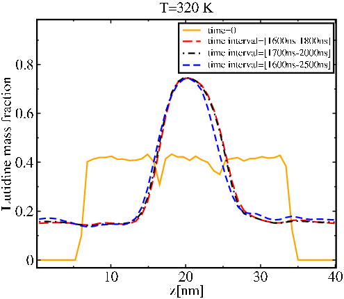
We simulated the 2,6-lutidine/water mixture in the NpT ensemble for various temperatures; the simulation setting is given in Sec. II.1. The time evolution of the local mass density of 2,6-lutidine for several temperatures are presented in Fig. 3. The plots show clearly a phase separated system at and and a homogeneous mixture at . The actual equilibration time is determined with the time at which not only the density profiles remain the same within the statistical errors, but also the energies and all hydrogen bonds become stable. Fig. 4 presents the density profiles averaged over different time intervals after the equilibration, for two temperatures. Depending on temperature, stable equilibrium structures were reached after . The simulations took several months, with average run of for each temperature.

The results of the simulation are reported in the next section.
III Simulation results
III.1 Phase behaviours of the 2,6-lutidine/water mixture near the lower critical point
Fig. 2 shows the snapshots of the initial configuration for all simulations (top) and simulation results for temperatures K (center) and K (bottom). The snapshots show that the two fluids mix at K, while they phase separate at the higher temperature K. In order to assure that the phase separation is not effected by the initial configuration, the simulations at these two temperatures were redone with different initial configurations. Although we used a mixed phase as the initial configuration for the higher temperature K and a phase-separated initial configuration for the lower temperature K, the same final configurations as given in Fig. 2 (bottom and center respectively) were reproduced.

To quantify the phase separation, the mass fraction of 2,6-lutidine has been calculated as a function of -coordinate from simulations at different temperatures, see Fig. 5. ’Classical‘ theories for the interface separating two coexisting phases such Cahn and Hilliard [70] or Landau-Ginzburg theory, predict a hyperbolic-tangent shaped interfacial density profiles. This has later been verified in simulations of interfaces [76, 66, 71, 72, 73, 74, 75, 77, 78]. Since there are two interfaces in the present system, we fit the density profile to the function
| (7) |
with and being the mass fractions of 2,6-lutidine in the lutidine-rich and lutidine-poor phases. is a measure of the width of the interface (softness of the transition between the two regions) and is proportional to the correlation length , which is defined from the decay of the density-density correlation function. is half width of the lutidine-rich region and is center of the lutidine-rich phase. Fits Eq. 7 to the profiles are shown in Fig. 5 as dashed lines. The parameters obtained from the fits are given in Table. 4 while the coexistence curve obtained from the data in the table is shown in Fig. 6. In order to compare with experiments [22, 24, 25] one may need to convert between mass fractions and mole fractions. The appropriate equations for this are
| (8) |
where indicates mass and mole fractions respectively, while refers to water and 2,6-lutidine molecules with molar masses . The mass and mole fractions of 2,6-lutidine are shown in the left and right vertical axes in Fig. 5 for several temperatures, and by circles and squares in Fig. 6.
| T[K] | lutidine-rich phase | lutidine-poor phase | [nm] | c [nm] |
|---|---|---|---|---|
| 315 | 0.67 0.03 | 0.185 0.006 | 3. 0.8 | 3.4 0.2 |
| 318 | 0.71 0.008 | 0.181 0.005 | 1.82 0.2 | 3.75 0.02 |
| 320 | 0.75 0.01 | 0.155 0.004 | 1.8 0.3 | 4.20 0.02 |
| 325 | 0.78 0.007 | 0.138 0.01 | 1.6 0.2 | 4.39 0.03 |
| 330 | 0.798 0.01 | 0.112 0.002 | 1.38 0.2 | 5.05 0.01 |
| 340 | 0.828 0.002 | 0.090 0.01 | 1.18 0.1 | 5.25 0.02 |
| 360 | 0.847 0.002 | 0.082 0.01 | 1.08 0.02 | 5.49 0.001 |
| 380 | 0.849 0.003 | 0.077 0.01 | 1.05 0.05 | 5.58 0.02 |

When is approached from above, increases and will eventually not be much smaller than .
Then, the system will be too small to accommodate a saturated lutidine-rich phase. We note that
this starts to occur at K. This makes it difficult to determine the lutidine mass fraction in the lutidine-rich phase. At higher temperatures we could just read off the value of from the flat part of the mass fraction profiles.
The alternative way to determine is by fitting the parameters in Eq. 7 to simulation data. At high temperatures, this method gives the same values for as the ones extracted from the flat parts of the mass fraction profiles, whereas for and K it gives the values that are higher than the maxima in Fig. 5. The question is now whether this procedure could be trusted or not. First we note that the fit of the mass fraction profile to the functional form of Eq.7 looks very good. We tested the validity of this procedure further
by running simulations of a smaller system in which the width of the lutidine-rich region is about one third of the present one, at two temperatures and K. For the smaller system the density profiles do not exhibit flat regions corresponding to the lutidine-rich phases at these temperatures, unlike the original simulations. By fitting the mass fraction profiles to Eq. 7, we do however obtain
the same values for in the lutidine-rich regions as in the large system at the same temperatures, despite that the maximum of the mass fraction profiles are about smaller compared to the larger system.
Although we do know that it eventually may break down close to , but we are clearly not close enough for that.
Now, we turn to the critical properties of the system. We fully realize that an
accurate calculation of critical exponents and would require simulations
closer to , larger systems and a finite-size scaling analysis [79].
This would for the present fairly complicated system call for an unjustifiable
amount of computer resources. Therefore, based on our simulations, the calculated
exponents are obtained within certain amount of statistical errors.
As mentioned earlier, in order to minimize the finite-size effects
we limited our simulations to the range of temperatures further away from , for which the bulk correlation length of the mixture is distinctively smaller
than the linear dimension of the simulation box (see below) and the order parameter is relatively large. Under such conditions we do not expect the mean field behaviour
to occur [80, 81]. On the other hand, in this temperature range the corrections to the critical scaling are relevant and therefore we will employ them.
The critical point and the shape of the coexistence curve were determined by using well established procedures [82, 83, 84, 85, 86, 87, 88].
By employing the Wegner expansion [89], the order parameter (OP) which in this case is the mass fraction difference of lutidine in the rich and poor phases , can be written as
| (9) |
where . The rectilinear diameter can be similarly expressed as
| (10) |

In Eqs. 9-10 is the mass fraction of lutidine at the critical point, , and , are non-universal constants, while , and are universal critical exponents. For the Ising universality class relevant for the present study, the exponents are approximately , and [90, 91, 92, 93]. We fitted the obtained and from the simulations (Table. 4) to Eqs. 9-10. This resulted in the values of and and in the first line of Table. 5, when the three exponents were fixed to their Ising universality class values. The results of the fit corresponding to the first row of the Table. 5 are shown in Fig. 7 together with the experimental coexistence curve [23]. The obtained curve exhibits a slight shift to the right as compared to the experimental one. In Fig. 8 we show the OP as a function of the reduced temperature together with the fit to Eq. 9 with (left panel) and without (right panel) correction-to-scaling term. One can see that the OP is fitted quite well to the power law with the 3D Ising exponent (after ignoring two data points furthest away from ); including the correction-to scaling makes this fitting work also for temperatures further away from . As a check for consistency of our estimates, we performed fitting treating the exponent as a free parameter. This fit provides a value of that is only slightly different from the Ising exponent (see Table. 5).
We also estimated the temperature interval in which the UCP of the mixture is located. This was done by running simulations (with the similar setting as in the original ones) for a smaller system () at several higher temperatures. The simulations data show a phase-separated mixture at K, while a mixed liquid phase at . This indicates that UCP is located between - K, in agreement with experiments [22, 25, 27].


| [K] | ||||||||
|---|---|---|---|---|---|---|---|---|
| 0.326 (fix) | 0.1 (fix) | 0.5 (fix) | 310.8 0.5 | 0.42 0.002 | -2.84 0.1 | 2.6 0.1 | 2.18 0.05 | -1.95 0.1 |
| 0.34 0.06 | 0.1 (fix) | 0.5 (fix) | 310.5 1.5 | 0.41 0.01 | -2.9 0.2 | 2.7 0.2 | 2.3 0.5 | -2.2 0.7 |
III.2 The surface tension and the correlation length of 2,6-lutidine/water mixture


We computed the surface tension in the phase-separated system (above the LCT) as a function of temperature from the simulations as an integral of the difference between the normal and tangential components of the pressure (stress) tensor across the interface [94]; the result as a function the reduced temperature is plotted in Fig. 9. The surface tension and the correlation length have similar scaling behaviour as the OP, but with different universal exponents [95, 85, 96, 94]
| (11) |
| (12) |
where , and , are non-universal constants.
We fitted the simulation data of and to these expressions
using the value of fixed to its Ising universality class value.
In the Tables. 6-7, the first rows are fits with the exponents and fixed to the Ising universality class values, while the second rows show the fits with and as free fitting parameters. The last rows show fits obtained by imposed as estimated from the coexistence curve fit (Table. 5).
All these different way of fitting give similar values of parameters.
The fits to Eqs. 11-12 with parameters from first rows of Tables. 6-7 (fixed critical exponents and )
are shown in Figs. 9-10.
| [mN/m] | [mN/m] | [K] | ||
|---|---|---|---|---|
| 1.26 (fix) | 0.5 (fix) | 56.8 3 | -85.7 7 | 311.45 0.75 |
| 1.28 0.18 | 0.5 (fix) | 65 23 | -100 40 | 311.5 2.5 |
| 1.35 0.11 | 0.5 (fix) | 73 16 | -113 27 | 310.5 1.5 (fix) |
| [nm] | [nm] | [K] | ||
|---|---|---|---|---|
| 0.63 (fix) | 0.5 (fix) | 0.036 0.013 | 0.77 0.05 | 314 0.4 |
| 0.62 0.02 | 0.5 (fix) | 0.06 0.04 | 0.67 0.09 | 313.3 0.8 |
| 0.68 0.05 | 0.5 (fix) | 0.087 0.003 | 0.48 0.07 | 310.5 1.5 (fix) |
| Exponent | Simulation | Ising | Ising | Mean-field |
|---|---|---|---|---|
| Order parameter, | 0.326 | 0.125 | 0.5 | |
| Correlation length, | 0.63 | 1 | 0.5 | |
| Surface tension, | 1.26 | 1 | 1.5 |
III.3 Interactions between water and 2,6-lutidine in the mixture


Fig. 11 (left) shows the interaction energy between water and 2,6-lutidine molecules per lutidine molecule for different temperatures. The figure indicates that the attraction between water and lutidine becomes stronger upon decreasing temperature. Fig. 11 (right) shows the number of hydrogen bonds between water and 2,6-lutidine molecules per lutidine molecule. From the figure it is seen that upon decreasing temperature the number of hydrogen bonds between water and 2,6-lutidine molecules increases, in line with the behaviour seen in Fig. 11 (left).
IV Conclusion
In this study, we have proposed an atomistic description of the 2,6-lutidine molecule which we have shown is able to successfully describe bulk 2,6-lutidine liquid. We then have employed this model together with the TIP4P/2005 water model to study the phase behaviour of 2,6-lutidine/water mixture near the LCP. We conclude that by using these models for molecules it is possible to describe the critical properties of the mixture well. From the density profiles computed in simulations we have obtained phase diagram of the mixture with the lower critical temperature , which is just a couple of degrees higher than the experimental value [22, 24, 25, 27]. We have found that the UCP is located between - K, in agreement with experiments [22, 25, 27]. We have computed the order parameter, the surface tension and the correlation length as a function of temperature. As expected, the order parameter and the surface tension vanish upon approaching the LCP from above, while the correlation length increases. Moreover, we have found that close to the temperature dependence of these quantities is well described by power laws. The calculated exponents deviate less than about from those of the 3D Ising universality class [90, 91, 92, 93] to which the studied system belongs. However, the estimated errors are clearly larger than this. A more accurate calculation of the critical exponents and of Tc would require simulations closer to Tc , larger systems and a finite-size scaling analysis [79].
V Acknowledgments
The work has been supported by the Swedish National Infrastructure for Computing (SNIC) with computer timed for the Center for High Performance Computing (PDC) and High Performance Computing Center North (HPC2N) and by National Science Center (Harmonia Grant No. 2015/18/M/ST3/00403). FP and OE would like to thank J. Lidmar and M. Wallin for useful discussions. FP would like to acknowledge E. Lindahl and B. Hess and their group members for helpful discussions during the meetings in SciLifeLab, and from L. Lundberg for quantum chemistry simulations of lutidine molecule.
References
- [1] J. Hirschfelder, D. Stevenson, and H. Eyring, J. Chem. Phys. 5, 896 (1937).
- [2] T. Narayanan and A. Kumar, Physics Reports 249(3), 135 (1994).
- [3] J. S. Walker and C. A. Vause, Phys. Lett. A 79, 421 (1980).
- [4] J. S. Walker and C. A. Vause, Sci. Am. 256(5), 98-105 (1987).
- [5] J. S. Walker and C. A. Vause, J. Chem. Phys. 79, 2660 (1983).
- [6] N. G. Almarza, Phys. Rev. E 86, 030101 (2012).
- [7] I. V. Brovchenko and A. V. Oleinikova, J. Chem. Phys. 106, 7756 (1997).
- [8] A. E. Robertson, D. H. Phan, J. E. Macaluso, V. N. Kuryakov, E. V. Jouravleva, C. E. Bertrand, I. K. Yudin, and M. A. Anisimov, Fluid Phase Equilibria 407, 243 (2016).
- [9] I. V. Brovchenko and B. Guillot, Fluid Phase Equilibria 183-184, 311 (2001).
- [10] M. D. Smith, B. Mostofian, L. Petridis, X Cheng and J. C. Smith, J. Phys. Chem. B. 120, 740 (2016).
- [11] D. W. Pohl and W. I. Goldburg, Phys. Rev. Lett. 48, 1111 (1982); L. Siegl and W. Fenzel, ibid 57, 2191 (1986).
- [12] B. J. Frisken, F. Ferri, and D. S. Cannel, Phys. Rev. Lett. 66, 2754 (1991).
- [13] M. L. Broide, Y. Garrabos, and D. Beysens, J. Chem. Phys. 47, 3768 (1993).
- [14] P. D. Gallagher and J. V. Maher, Phys. Rev. A 46, 2012 (1992).
- [15] D. Beysens and D. Estv̀e, Phys. Rev. Lett. 54, 2123 (1985); D. Beysens and T. Narayanan, J. Stat. Phys. 96, 997 (1999).
- [16] M. L. Kurnaz and J. V. Maher, Phys. Rev. E 51, 5916 (1995).
- [17] M. L. Kurnaz and J. V. Maher, Phys. Rev. E 55, 572 (1997).
- [18] C. Hertlein, L. Helden, A. Gambassi, S. Dietrich, and C. Bechinger, Nature 451, 172 (2008).
- [19] A. Gambassi, A. Maciołek, C. Hertlein, U. Nellen, L. Helden, C. Bechinger, and S. Dietrich, Phys. Rev. E 80, 061143 (2009).
- [20] U. Nellen, L. Helden, C. Bechinger, EPL 88, 26001 (2009).
- [21] V. D. Nguyen, S. Faber, Z. Hu, G. H. Wegdam, and P. Schall, Nat. Commun. 4, 1584 (2013).
- [22] R. J. L. Andon and J. D. Cox, J. Chem. Soc., 4601-4606 (1952).
- [23] R. M. Stephenson, J. Chem. Eng. Data 38(3), 428-431 (1993).
- [24] C. A. Grattoni, R. A. Dawe, C. Yen Seah, and J. D. Gray, J. Chem. Eng. Data. 38, 516-519 (1993).
- [25] J. D. Cox and E. F. G. Herington, Trans. Faraday Soc. 52, 926-930 (1956).
- [26] Y. Jayalakshmi, J. S. V. Duijneveldt, and D. Beysens, J. Chem. Phys. 100, 604 (1993).
- [27] A. W. Francis, Critical Solution Temperatures, Advances in Chemistry Series 31; American Chemical Society: Washington DC, (1961).
- [28] A. W. Loven and O. K. Rice, Trans. Faraday Soc. 59, 2723 (1963).
- [29] E. Gülari, A. F. Collings, R. L. Schmidt, and C. J. Pings, J. Chem. Phys. 56, 6169 (1972).
- [30] V. A. Levchenko and V. P. Voronov, Int. J. Thermophys. 14, 221 (1993).
- [31] S. Z. Mirzaev, R. Behrends, T. Heinburg, J. Haller, and U. Kaatze, J. Chem. Phys. 124, 144517 (2006).
- [32] K. Sadakane, N. Iguchi, M. Nagao, H. Endo, Y. B. Melnichenko and H. Seto, Soft Matter 7(16), 1334 (2011).
- [33] K. Sadakane, A. Onuki, K. Nishida, S. Koizumi and H. Seto, Phys. Rev. Lett. 103, 167803 (2009).
- [34] J. Leys, D. Subramanian, E. Rodezno, B. Hammouda and M. A. Anisimov, Soft Matter 9, 9326 (2013).
- [35] K. Sadakane, H. Endo, K. Nishida and H. Seto, J. Solution Chem. 43, 1722 (2014).
- [36] A. Onuki and H. Kitamura, J. Chem. Phys. 121, 3143 (2004).
- [37] F. Pousaneh and A. Ciach, Soft Matter 10, 8188 (2014).
- [38] U. Nellen, J. Dietrich, L. Helden, S. Chodankar, K. Nygard, J. F. van der Veen and C. Bechinger, Soft Matter 7, 5360 (2011).
- [39] A. Gambassi, M. Oettel and S. Dietrich, Europhys. Lett. 95, 60001 (2011).
- [40] A. Ciach and A. Maciołek, Phys. Rev. E 81, 041127 (2010).
- [41] F. Pousaneh, A. Ciach and A. Maciołek, Soft Matter 8, 3567 (2012).
- [42] D. Van Der Spoel, E. Lindahl, B. Hess, G. Groenhof, A. E. Mark, and H. J. C. Berendsen, J. Comput. Chem. 26(16), 1701 (2005).
- [43] N. Schmid, A. P. Eichenberger, A. Choutko, S. Riniker, M. Winger, A. E. Mark, and W. F. van Gunsteren, Eur. Biophys. J. 40, 843-856 (2011).
- [44] T. Darden, D. York, and L. Pedersen, J. Chem. Phys. 98(12), 10089 (1993).
- [45] G. Bussi, D. Donadio, and M. Parrinello, J. Chem. Phys. 126, 014101 (2007).
- [46] M. Parrinello and A. Rahman, J. Appl. Phys. 52, 7182-7190 (1981).
- [47] B. Hess, H. Bekker, H. J. C. Berendsen, and J. G. E. M. Fraaije, J. Comput. Chem. 18, 1463-1472 (1997).
- [48] J. L. F Abascal and C. Vega, J. Chem. Phys. 123, 234505 (2005).
- [49] W. Humphrey, A. Dalke and K. Schulten, J. Mol. Graphics 14, 33 (1996).
- [50] T. Giorgino, Comput. Phys. Commun. 185, 317 (2014).
- [51] W. V. Steele, R. D. Chirico, A. Nguyen, and S. E. Knipmeyer, J. Chem. Thermodyn. 27, 311-334 (1995).
- [52] M. S. Bakshi, J. Chem. Soc., Faraday Trans. 89, 3049 (1993).
- [53] J. O. Jenkins and J. W. Smith, J. Chem. Soc. B, 1538-1541 (1990).
- [54] T. Mainzer-Althof and D. Woermann, Ber. Bunsen-Ges. Phys. Chem. 101 , 1014 (1997).
- [55] V. K. Shen, D. W. Siderius, and W. P. Krekelberg, NIST Standard Reference Simulation Website, NIST Standard Reference Database.
- [56] M. Feig, Modelling solvent environment: applications to simulations of biomolecules, Wiley-VCH, Weinheim, (2010).
- [57] P. H. Berens, D. H. J. Mackay, G. M. White, and K. R. Wilson, J. Chem. Phys. 79, 2375 (1983).
- [58] Q. Waheed and O. Edholm, J. Chem. Theory Comput. 7, 2903-2909 (2011).
- [59] M. P. Allen and D. J. Tildesly, Computer simulation of liquids, Oxford Science Publications, Oxford (1987).
- [60] W. M. Haynes (ed.), CRC Handbook of Chemistry and Physics, 94th edition. CRC Press, Boca Raton, (2013).
- [61] R. G. Mortimer, Physical Chemistry , Elsevier Academic Press, San Diego, California, 3rd edition, (2008).
- [62] N. O. Smith, J. Chem. Educ. 42(12), 654 (1965).
- [63] R. Godawat, S. N. Jamadagni, J. R. Errington and S. Garde, Ind. Eng. Chem. Res., 47(10), 3582 (2008).
- [64] Z. Shi, P. G. Debenedetti and F. H. Stillinger, J. Chem. Phys. 134, 114524 (2011).
- [65] L. G. MacDowell, V. K. Shen an J. R. Errington, J. Chem. Phys. 125 034705 (2006).
- [66] G. A. Chapela, G. Saville, S. M. Thompson, and J. S. Rowlinson, J. Chem. Soc., Faraday Trans. 2, 73, 1133 (1977).
- [67] C. D. Holcomb, P. Clancy, and J. A. Zollweg, Mol. Phys. 78, 437 (1993).
- [68] L. J. Chen, J. Chem. Phys. 103, 10214 (1995).
- [69] A. Trokhymchuk and J. Alejandre, J. Chem. Phys. 111(18), 8510 (1999).
- [70] J. W. Cahn and J. E. Hilliard, J. Chem. Phys. 28, 258 (1958).
- [71] M. Müller, K. Binder, and W. Oed, J. Chem. Soc., Faraday Trans. 91, 2369 (1995).
- [72] M. Mecke, J. Winkelmann, and J. Fischer, J. Chem. Phys. 107, 9264 (1997).
- [73] H. Watanabe, N. Ito, and C. Hu, J. Chem. Phys. 136, 204102 (2012).
- [74] I. Omelyan, F. Hirata, and A. Kovalenko, Phys. Chem. Chem. Phys. 7, 4132-4137 (2005).
- [75] F. J. Blas, L. G. MacDowell, E. D. Miguel, and G. Jackson, J. Chem. Phys. 129, 144703 (2008).
- [76] J. E. Inglesfield, Cohesion and Structure of Surfaces, Vol 4 edited by K. Binder, M. Bowker, J. E. Inglesfield and P. J. Rous, Elsevier Science, (1995).
- [77] T. H. Yang and C. Pan, Intern. Journ. of Heat and Mass Transfer. 48, 3516-3526 (2005).
- [78] S. Eckelsbach and J. Vrabec, Phys. Chem. Chem. Phys. 17, 27195-27203 (2015).
- [79] M. N. Barber in Phase Transitions and Critical Phenomena, Volume 8, edited by C. Domb and J. L. Lebowitz, Academic Press, New York, (1983), V. Privman, in Finite Size Scaling and Numerical Simulation of Statistical Systems, edited by V. Privman, World Scientific, Singapore, (1990).
- [80] K. Mon and K. Binder, J. Chem. Phys. 96, 6989 (1994).
- [81] A. Z. Panaglotopoulos, International Journal of Thermophysics 15, 1057 (1994).
- [82] Y. Guissani and B. Guillot, J. Chem. Phys. 98(10), 8221 (1993).
- [83] F. Vnuk and J. Chem. Soc., Faraday Trans. 2, 79, 41-55 (1983).
- [84] D. Beysens, J. Chem. Phys. 71, 2557 (1979).
- [85] A. Aharony and G. Ahlers, Phys. Rev. Lett. 44, 782 (1980).
- [86] C. Bagnuls and C. Bervillier, Phys. Rev. B 24, 1226-1235 (1981).
- [87] V. A. Durov, in: J. Samios, V.A. Durov (Eds.), Novel Approaches to the Structure and Dynamics of Liquids: Experiments, Theories and Simulations , NATO Science Series. II, Mathematics, Physics and Chemistry, Kluwer, Dortrecht, 17-40 (2004).
- [88] C. Vega, J. L. F. Abascal, and I. Nezbeda, J. Chem. Phys. 125, 034503 (2006).
- [89] F. Wegner, Phys. Rev. B 5(11), 4529 (1972).
- [90] A. Pelissetto and E. Vicari, Phys. Rep. 368, 549 (2002).
- [91] M. Gitterman and V. Halpern, Phase Transition: A Brief Account with Modern Applications, World Scientific, (2004).
- [92] D. C. Mattis, R. H. Swendsen, Statistical Mechanics Made Simple, 2nd ed. World Scientific, (2008).
- [93] J. G. Brankov, D. M. Danchev, and N. S. Tonchev, Theory of Critical Phenomena in Finite-size Systems: Scaling and Quantum Effects, Singapore: World Scientific, (2010).
- [94] J. S. Rowlinson and B. Widom, Molecular Theory of Capillarity, Oxford University Press, (1982).
- [95] W. Rathjen and J. Straub, Surface tension and refractive index of six refrigerants from triple point up to critical point, Proc. 7th Symposium on Thermophysical Properties, Washingron, USA, May 10-12, (1977).
- [96] D. Beysens, A. Bourgou, and P. Calmettes, J. Phys. Rev A. 26, 3589 (1982).