How to Measure Black Hole’s Mass, Spin and Direction of Spin Axis in Kerr Lens Effect 1: test case with simple source emission near BH

Our target phenomenon is a single burst-like (short duration) isotropic emission by a source that is much smaller than its host BH. This is modeled as a point-like source that moves near the BH and emits light rays in all directions within a duration much shorter than a typical dynamical time scale of the system composed of the source and the BH (e.g. the Keplerian time scale of the source around BH). Further, we assume that the environment around the BH is transparent, at least in the frequency band of observation. Note that the details of the intrinsic structure of the source is outside the scope of this paper, and we assume such a simple emission occurs in the transparent environment around BH. We focus on how the gravitational lens effect of the Kerr BH appears in observable quantities of light rays that are emitted by the source and received by a rest observer distant from the BH.

On these assumptions, let us note that an example of a transparent environment has been recognized for the massive BH candidate at the center of our galaxy, Sagittarius A^∗ (Sgr A^∗) [3, 7, 21]. Radio observational data of Sgr A^∗ for a rather wide band range indicate the disappearance of plasma scattering effects at high frequency ($>230$ GHz) radio waves, which implies a transparent environment around the BH for such high frequency radio photons [3, 7, 21]. Further, it is also reported that intermediate mass BH candidates seem to exist in the central region of our galaxy [19]. Such an intermediate mass BH candidate does not form a binary with some other body, but it is recognized by a significant (large acceleration) motion of gas cloud around a dark compact region, which is consistent with assuming an intermediate mass BH in the dark compact region [19]. We may expect that such an intermediate mass BH, if it exists, wears a transparent and inactive environment.

Here note that the estimated mass of Sgr A^∗ is about $4\times 10^{6}M_{\odot}$ [2], and that of the intermediate mass BH is about $10^{5}M_{\odot}$ [19], where $M_{\odot}\simeq 2\times 10^{30}$ kg is the mass of the Sun. Therefore, gas clouds and celestial bodies whose mass is about $M_{\odot}$ are much smaller than those BHs. Then, let us consider the case that a gas cloud or a dark celestial body of stellar mass falls toward the BH and emits a short duration emission in all directions (due, e.g., to some shock formation or disruption event). Such a case may be effectively described by our assumptions or by some appropriate summation of our simple source emission. Anyway, the detail of the source’s structure is outside the scope of this paper and will be properly treated in another paper. Our interest, in this paper, is in the theoretical properties of the Kerr BH lens effect under our assumptions described in the first paragraph.

Let us make a comment on the terminology. The term “strong gravitational lens effect” is already used in, e.g., the survey of galaxy distribution, dark matter distribution, and so on. The meaning of this term in those research fields is the lens effect of a cluster of masses (not necessarily BHs) that produces the multi-image of a source (e.g. galaxy) behind the cluster. This usage of “strong gravitational lens effect” includes the effect of mass, but not the effect of a BH’s spin. However, we are interested in the lens effect of a spinning BH, which shall include the effect not only of the mass but also of the spin of the BH. Therefore, we use the term Kerr BH lens effect (or Kerr lens effect) for the lens effect produced by the mass and spin of a Kerr BH.

To describe Kerr spacetime, we use Boyer-Lindquist (BL) coordinates $(t,r,\theta,\varphi)$ throughout this paper. The metric components $g_{\mu\nu}$ are read from the line element of spacetime,

and the time coordinate $t$, the BH’s mass $M$ and spin parameter $a:=J/M$ (where $J$ is the spin angular-momentum) are measured in the dimension of length. Instead of $a$, we use the dimensionless spin parameter $\chi:=a/M$, when it is convenient for the line of thought. In some figures shown later, we project 4-dimensional null geodesics onto 3-dimensional screen spanned by

In this 3D screen, the $z$-axis corresponds to the axis of the BH’s spin.

The radius of the BH horizon is $r_{\rm BH}=M\bigl[\,1+\sqrt{1-\chi^{2}}\,\bigr]$, and the ergosurface is $r_{\rm erg}(\theta)=M\bigl[\,1+\sqrt{1-\chi^{2}\cos^{2}\theta}\,\bigr]$. The BH’s spin is a rigid rotation, due to the rigidity theorem, with angular velocity $\omega_{\rm BH}=\omega(r_{\rm BH},\pi/2)=\chi/(2r_{\rm BH})$. Without loss of generality, we can set $0\leq\chi<1$, where the upper bound is due to the existence of the BH horizon, and the non-negativity of $\chi$ corresponds to the direction of BH spin given by $\omega_{\rm BH}\geq 0$. We do not need to consider the opposite direction of spin because of the axisymmetry of Kerr spacetime.

The zero-angular-momentum-observer (ZAMO) is defined as the one whose 4-velocity $u_{\rm zamo}^{\mu}$ is perpendicular to the spacelike hypersurface at $t=$ constant,

Although ZAMO has, by definition, no angular-momentum with respect to the spacelike hypersurface at $t=$ constant, its 4-velocity, however, has a $\varphi$-component. This is understood as the effect of the rotation of spacetime itself, which is called the frame dragging effect of Kerr BH. The angular velocity of ZAMO measured in BL coordinates, $u_{\rm zamo}^{\varphi}/u_{\rm zamo}^{t}=\omega$, is regarded as the angular velocity of the frame dragging effect measured in BL coordinates.

The timelike and spacelike Killing vectors are, respectively in BL coordinates, $\xi_{\rm(t)}^{\mu}=(1,0,0,0)$ and $\xi_{\rm(\varphi)}^{\mu}=(0,0,0,1)$. The metric $g_{\mu\nu}$ satisfies the Killing equations, $\mathcal{L}_{\xi_{\rm(t)}}g_{\mu\nu}=0\,,\,\mathcal{L}_{\xi_{\rm(\varphi)}}g_{\mu\nu}=0$, where $\mathcal{L}$ denotes the Lie derivative. And, Kerr spacetime is of Petrov type D, which possesses 2 principal null vectors (a kind of eigenvector of Weyl curvature tensor), $m^{\mu}$ and $n^{\mu}$. These produce a Killing tensor that is, in BL coordinates, $\Xi_{\mu\nu}=(m_{\mu}n_{\nu}+m_{\nu}n_{\mu})\Sigma+r^{2}g_{\mu\nu}$, where $m_{\mu}=(1,-\Sigma/\Delta,0,-a\sin^{2}\theta)$ and $n_{\nu}=(\Delta/(2\Sigma),1/2,0,[\Delta/(2\Sigma)]a\sin^{2}\theta)$. The Killing tensor equation $\Xi_{(\mu\nu;\alpha)}=0$ holds, where the semicolon “ ; ” in the subscript denotes the covariant derivative with respect to $g_{\mu\nu}$. These Killing fields, $\xi_{\rm(t)}$, $\xi_{\rm(\varphi)}$, and $\Xi$, express some symmetries of Kerr spacetime that produce some constants of motion of geodesics, and are used in Sect.3 to derive the formulas of observable quantities.

By the Kerr lens effect, the light ray winds around the BH before reaching the distant rest observer. An arbitrary number of windings around the BH are possible by tuning the values of the impact parameters of the light ray. In this paper, we focus on the 2 light rays that reach the distant observer earliest and secondary temporally. We call these rays, respectively, the primary ray (p-ray) and secondary ray (s-ray). Some numerical examples of the orbits of these rays (solutions of null geodesic equations) are shown in Fig.1, which depicts not only the p-ray and the s-ray but also other 2 rays of higher winding number that reach the same rest observer. (The detail is explained in Sect.3.)

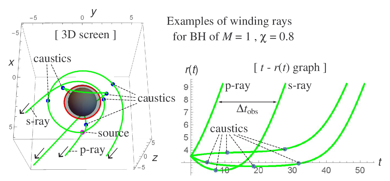
As explained in Sect.1, the observable quantities that we focus on are the delay $\Delta t_{\rm obs}$ between the detection time of the p-ray $t_{\rm obs(p)}$ and that of the s-ray $t_{\rm obs(s)}$, and the ratio $\mathcal{R}_{\rm obs}$ of the observed specific flux of the s-ray $F_{\rm obs(s)}$ to that of the p-ray $F_{\rm obs(p)}$:

The dimensions of $F_{\rm obs}$ are W/(m² Hz) in MKS units, where 1/m² denotes per unit spatial area perpendicular to the observer and 1/Hz denotes per unit observed frequency which is the meaning of “specific”. Under the assumptions introduced in Sect.2.1, the time delay $\Delta t_{\rm obs}$ and specific flux ratio $\mathcal{R}_{\rm obs}$ are regarded as functions of some parameters.

The time delay $\Delta t_{\rm obs}$ is regarded as a function of following parameters,

where the emission time is set to 0 ($t_{\rm emi}=0$) and the distant limit of the observer ($r_{\rm obs}\to\infty$) is supposed as mentioned in Sect.2.1. The parameters $(\theta_{\rm obs},\varphi_{\rm obs})$ and $x^{\mu}_{\rm emi}$ determine the relative location among the BH, source and distant observer.

Note that, by the axisymmetry of Kerr spacetime, we can rotate the BL coordinates in the $\varphi$-direction so as to make the new azimuthal angles of the observer and source $\varphi^{\prime}_{\rm obs}=0$ and $\varphi^{\prime}_{\rm emi}=-\varphi_{\rm obs}$. However, for the convenience of our numerical calculation, we fix the source’s azimuthal coordinate at $\varphi_{\rm emi}=0$ and let the observer’s azimuthal coordinate $\varphi_{\rm obs}$ be a free parameter. Also, it is worth emphasizing that the zenithal angle $\theta_{\rm obs}$ is the direction angle of the BH’s spin axis seen from the observer (the angle between the line of sight and the spin axis).

Once the relative location is fixed, the null geodesic equation can be solved and the orbits of the p-ray and the s-ray are specified. Then, the detection times $t_{\rm obs(p)}$ and $t_{\rm obs(s)}$ are determined, and the time delay $\Delta t_{\rm obs}$ can be read from the numerical result as shown in the right-hand panel of Fig.1. This $\Delta t_{\rm obs}$ may be roughly estimated as $\Delta t_{\rm obs}\sim\alpha 2\pi r_{\rm emi}$, where $0\lesssim\alpha\lesssim 1$, and $\alpha\sim 1$ for $\varphi_{\rm obs}\sim 0$ (the emission event is in front of the BH seen from the observer) and $\alpha\sim 0$ for $\varphi_{\rm obs}\sim\pi$ (the emission event is behind the BH seen from the observer). For the example in Fig.1, $(M,\chi,r_{\rm emi})=(1\,,\,0.8\,,\,2.2\,r_{\rm BH})$, this estimation formula gives $\Delta t_{\rm obs}\sim 4.4\pi M(1+\sqrt{1-\chi^{2}})\simeq 22$ which is roughly consistent with the value of $\Delta t_{\rm obs}$ read from the right-hand panel of Fig.1.

Next, the observed specific fluxes of the p-ray and the s-ray, $F_{\rm obs(p)}$ and $F_{\rm obs(s)}$, are regarded as functions of the parameters in list (5) and

where, because the isotropic emission is assumed as mentioned in Sect.2.1, the emission intensity $I_{\rm emi}(\nu_{\rm emi})$ depends only on the emission frequency $\nu_{\rm emi}$ and not on the emission direction. The dimensions of $I_{\rm emi}(\nu_{\rm emi})$ are W/(m² Hz  ste-rad) in MKS units, where 1/m² denotes per unit spatial area perpendicular to the source, 1/ste-rad denotes per unit solid-angle seen from the source and 1/Hz denotes per unit frequency measured at the source. Further, $F_{\rm obs}$’s dependence on $u_{\rm emi}^{\mu}$ is due to the kinetic (special relativistic) Doppler effect on the light ray. Since the kinetic Doppler effect is determined by the relative velocity between the source and ray, the strength of the kinetic Doppler effect is different between the p-ray and the s-ray. However, since the p-ray and the s-ray are emitted by the same source at the same time, the strength of gravitational Doppler effects on those rays are the same because the gravitational Doppler effect is determined by the gravitational potential at the emission.

There are 2 basic types of observation of the specific flux ratio $\mathcal{R}_{\rm obs}$:

Type LD (line detection):

Detect the p-ray and the s-ray at the same observation frequency $\nu_{\rm obs}$. In this case, generally, the emission frequency of the p-ray $\nu_{\rm emi(p)}$ and that of the s-ray $\nu_{\rm emi(s)}$ are different ($\nu_{\rm emi(p)}\neq\nu_{\rm emi(s)}$), because the strength of the kinetic Doppler effect on the p-ray is generally different from that on the s-ray.

Type LE (line emission):

Detect the p-ray and the s-ray at different observation frequencies, respectively, $\nu_{\rm obs(p)}$ and $\nu_{\rm obs(s)}$, so that the difference between $\nu_{\rm obs(p)}$ and $\nu_{\rm obs(s)}$ offsets the difference between the kinetic Doppler effects on those rays. This means that the emission frequencies of the p-ray and the s-ray coincide, $\nu_{\rm emi}(\nu_{\rm obs(p)})=\nu_{\rm emi}(\nu_{\rm obs(s)})$. This case corresponds to a line emission by the source.

It will be shown in Sect.3 that, while the ratio $\mathcal{R}_{\rm obs}^{\rm(LD)}$ of type LD depends on the functional form of $I_{\rm emi}(\nu_{\rm emi})$, the ratio $\mathcal{R}_{\rm obs}^{\rm(LE)}$ of type LE, however, does not depend on $I_{\rm emi}(\nu_{\rm emi})$.

We are studying a method of measuring the value of $(M,\chi,\theta_{\rm obs})$ by observing quantities $(\Delta t_{\rm obs},\mathcal{R}_{\rm obs})$ which are functions of many parameters in lists (5) and (6). Our theoretical principle of measuring $(M,\chi,\theta_{\rm obs})$ is simple, consisting of the following 3 steps:

Step 1 (BH measurement):

This step consists of theoretical and observational tasks.

Task of theory:

Theoretically calculate the values of $(\Delta t_{\rm obs},\mathcal{R}_{\rm obs})$ for various values of the parameters (5) and (6).

Task of observation:

Using an appropriate telescope, observe the values of $(\Delta t_{\rm obs},\mathcal{R}_{\rm obs})$ for 1 BH candidate as many times as possible.

Step 2 (BH measurement):

From the results of step 1, construct a table such as Table 1. In each row of this table, all sets of the values of parameters (5) and (6) in the right-hand slot predict the same value of observable quantities $(\Delta t_{\rm obs},\mathcal{R}_{\rm obs})$ in the left-hand slot.

Step 3 (BH measurement):

It is a fact that the parameters $(M,\chi)$ and the direction angle $\theta_{\rm obs}$ will not change for all observational data $(\Delta t_{\rm obs},\mathcal{R}_{\rm obs})$, because the target BH candidate is the same for all data. Hence, if we find only 1 set of values of $(M,\chi,\theta_{\rm obs})$ that is shared by all rows in Table 1, then the common values should be the true values of the mass, spin parameter, and direction angle of the BH candidate under observation.

The above method consisting of 3 steps is our principle for measuring the value of the BH’s parameters $(M,\chi)$ and the direction angle $\theta_{\rm obs}$ of the BH’s spin axis. Because the value of $(M,\chi)$ is determined by the observable quantities of the Kerr BH lens effect (one of the general relativistic effects), our method is regarded as one principle of direct BH measurement under the definition given at the beginning of Sect.1.

Note that, in the task of observation, we do not need the repetition of observation under the same relative location among the BH, source, and observer. In general, the value of $(\Delta t_{\rm obs},\mathcal{R}_{\rm obs})$ for 1 relative location differs from that for the other relative location. The point is that the number of rows in Table 1 becomes large by observing the value of $(\Delta t_{\rm obs},\mathcal{R}_{\rm obs})$ as many times as possible for various relative locations. The larger the number of rows in Table 1, the more certain the true value $(M_{\rm true},\chi_{\rm true},\theta_{\rm true})$.

Also note that, when the values of parameters (5) and (6) are given, the flux ratio $\mathcal{R}_{\rm obs}^{\rm(LD)}$ of the type LD observation differs from $\mathcal{R}_{\rm obs}^{\rm(LE)}$ of the type LE observation in general (but the time delay $\Delta t_{\rm obs}$ is common to both types of observation). Therefore, in the task of theory, we need to perform 2 calculations of $\mathcal{R}_{\rm obs}^{\rm(LD)}$ and $\mathcal{R}_{\rm obs}^{\rm(LE)}$ for each given value of parameters (5) and (6). Then, one of them should be selected (or their combination should be constructed) according to the real observational method used in the task of observation.

We consider the rest observer, $(r_{\rm obs},\theta_{\rm obs},\varphi_{\rm obs})=$ constant, whose velocity is $u_{\rm obs}^{\mu}=(1/\sqrt{|g_{tt}|},0,0,0)$ satisfying $u_{\rm obs\mu}u_{\rm obs}^{\mu}=-1$. As mentioned in Sect.2.1, we consider the distant observer, $r_{\rm obs}\to\infty$, whose velocity becomes

The velocity of our observer coincides with the timelike Killing vector, $u_{\rm obs}=\xi_{\rm(t)}$.

Although our ideal setup is the observer at $r_{\rm obs}\to\infty$, our numerical calculation will be performed with putting the rest observer at $r_{\rm obs}=100\,r_{\rm BH}$ which gives $100/99\,(\simeq 1.01)\leq 1/\sqrt{|g_{tt}|}\leq 50/49\,(\simeq 1.02)$. On the other hand, we will use Eq.(7) for $u_{\rm obs}^{\mu}$ in our numerical calculation. This implies that our numerical results of observable quantities, shown in Sect.4, include an intrinsic error of $1\%\sim 2\%$. However, this error does not affect the numerical results showing the potential detectability of our observable quantities.

Since we assume the duration of emission is short (burst-like), the p-ray and the s-ray are both regarded as 1 pulse made of photons. The 4-dimensional orbit of a light ray is a null geodesic of spacetime. To emphasize the behavior of light ray as a pulse, we use the term “light ray”. To emphasize the 4-dimensional orbit of a light ray, we use the term “null geodesic”. Then, we can say that any light ray propagates on a null geodesic.

Let $h$ denote an affine parameter measured in the length dimension, and let $x_{\rm ng}^{\mu}(h)$ be the spacetime position of a light ray on the null geodesic. The wave vector of a light ray is given by $K^{\mu}={\rm d}x_{\rm ng}^{\mu}(h)/{\rm d}h$, which must satisfy the null condition $K^{\mu}K_{\mu}=0$. Due to the stationarity and axisymmetry of Kerr spacetime, any light ray possesses 3 constants of motion $(\nu_{\rm obs},l_{\varphi},l_{\rm nor})$ given by $K^{\mu}$ and Killing fields,

which are conserved along the null geodesic, $K^{\mu}Q_{;\mu}=0$, where $Q=\nu_{\rm obs}\,,\,l_{\varphi}\,,\,l_{\rm nor}$.

Our setup (7) of $u_{\rm obs}^{\mu}$ means that the quantity $\nu_{\rm obs}$ is calculated from $u_{\rm obs}^{\mu}$ as $\nu_{\rm obs}=-K_{\mu}u_{\rm obs}^{\mu}$. This $\nu_{\rm obs}$ is the dimensionless frequency of a light ray observed by a rest observer at infinity ($r_{\rm obs}\to\infty$), where “dimensionless” denotes that $\nu_{\rm obs}$ is normalized by a fiducial frequency. The quantity $l_{\varphi}$ is the $\varphi$-component (toroidal component) of the orbital angular-momentum of a light ray, and the quantity $l_{\rm nor}$ relates to the norm of the orbital angular-momentum of a light ray. These components, $l_{\varphi}$ and $l_{\rm nor}$, are measured per unit energy of the ray, since the dimension of them is the length in natural units ($c=1\,,\,G=1$).

Note that the fiducial frequency for the normalization of $\nu_{\rm obs}$ can be chosen arbitrarily. For example, in MKS units, if we choose $300$GHz as the fiducial frequency, then the unit of length size in our numerical calculation becomes $c/(300$GHz$)=10^{-3}$m. If, conversely, we set the unit of length size to $r_{\rm BH}$, then the fiducial frequency becomes $c/r_{\rm BH}$.

Hereafter, for simplicity of calculations, we normalize the null geodesic by $\nu_{\rm obs}$ as

The spacetime position of a light ray, $x_{\rm ng}^{\mu}(\eta)$, is determined by the null geodesic equations, $k^{\alpha}k^{\mu}_{\phantom{\mu};\alpha}=0$, whose components in BL coordinates, together with the null condition $k_{\mu}k^{\mu}=0$, can be arranged as

where the auxiliary functions are $X(r)=(r^{2}+a^{2}-ab)/\Delta(r)$ and $Y(\theta)=a\sin^{2}\theta-b$, and the radial and zenithal effective potentials are

Note that the normic impact parameter $q$ appears only in the squared form, $q^{2}$. This means that the solution of the null geodesic equation, $k^{\mu}(\eta)$ and $x_{\rm ng}^{\mu}(\eta)$, does not depend on the signature of $q$. We set $q\geq 0$ throughout this paper. Also, in our numerical calculation, we set $\eta=0$ at the emission event of light rays: $x_{\rm emi}^{\mu}=x_{\rm ng}^{\mu}(0)$ and $k_{\rm emi}^{\mu}=k^{\mu}(0)$.

We can recognize from Eq.(10) that, given the emission event $x_{\rm emi}^{\mu}$ and the initial null vector $k_{\rm emi}^{\mu}$ at the emission, the values of impact parameters $(b,q)$ corresponding to $x_{\rm emi}^{\mu}$ and $k_{\rm emi}^{\mu}$ are determined by solving Eq.(10) algebraically for $(b,q)$. In our numerical calculation, we use Eq.(10) for the following 2 purposes: (i) to evaluate the values of impact parameters $(b,q)$ for given $x_{\rm emi}^{\mu}$ and $k_{\rm emi}^{\mu}$, and (ii) to judge whether or not the light ray of given $x_{\rm emi}^{\mu}$ and $k_{\rm emi}^{\mu}$ is to be absorbed eventually by BH. The criterion of the judgment is given by the effective potentials (11) as explained in Appendix A.

If one tries to integrate Eq.(10), then there arises the problem of how to choose the signatures of $k^{r}=\pm\sqrt{|V_{\rm eff}|}/\Sigma$ and $k^{\theta}=\pm\sqrt{|U_{\rm eff}|}/\Sigma$. We avoid this problem by using the Hamiltonian formalism of geodesics instead of Eq.(10). Define the Hamiltonian of a light ray by

where we regard the position $x_{\rm ng}^{\mu}(\eta)$ and the null 1-form $k_{\mu}(\eta)$ as the dynamical variables in the present Hamiltonian formalism. In Kerr spacetime, the components of the 1-form in BL coordinates are

where the $t$-component and $\varphi$-component are constant because of Eq.(8) and (9b). The Hamilton equations, ${\rm d}x_{\rm ng}^{\mu}(\eta)/{\rm d}\eta=\partial\mathcal{H}/\partial k_{\mu}$ and ${\rm d}k_{\mu}(\eta)/{\rm d}\eta=-\partial\mathcal{H}/\partial x_{\rm ng}^{\mu}$, are reduced to the following 6 simultaneous equations:

In these equations, no square root appears.

Note that the Euler-Lagrange equations given by the Lagrangian corresponding to the Hamiltonian (12) can be arranged to geodesic equations of the form (10). Also, note that the value of the Hamiltonian, $\mathcal{H}\propto k^{2}\equiv 0$, is conserved along the geodesic. Therefore, the null geodesic $x_{\rm ng}^{\mu}(\eta)$ is obtained automatically by solving Eq.(14) with the initial condition satisfying $k_{\rm emi}^{2}=0$. In our numerical calculation, the initial null 1-form $k_{\rm emi\,\mu}$ is constructed by making use of Eq.(10) as explained in Appendix A. Then, the null geodesics of the p-ray $x_{\rm ng(p)}^{\mu}(\eta)$ and the s-ray $x_{\rm ng(s)}^{\mu}(\eta)$, which connect the source and observer, are obtained by solving Eq.(14) numerically, and we can plot those solutions in the $t$-$r$ plane and read out the time delay $\Delta t_{\rm obs}$ as shown in Fig.1.

Given the observed frequency $\nu_{\rm obs}$ of a light ray detected by the observer, the emission frequency $\nu_{\rm emi}$ of the ray can be given by

where Eq.(13) is used. When the source is moving near the BH, we cannot identify which term in Eq.(15) is responsible for the gravitational or kinetic Doppler effect. Let us define the total-Doppler factor $\mathcal{D}$ as the ratio of $\nu_{\rm obs}$ to $\nu_{\rm emi}$,

This can be regarded as a function of the emission event $x_{\rm emi}^{\mu}$, the velocity of the source $u_{\rm emi}^{\mu}$, and the initial null vector of the light ray $k_{\rm emi}^{\mu}$. Thus, the value of $\mathcal{D}$ can be calculated numerically once the null geodesic that connects the source and observer is obtained numerically by the formulas shown in Sect.3.2. The values of $\mathcal{D}_{\rm(p)}$ of the p-ray and $\mathcal{D}_{\rm(s)}$ of the s-ray are generally different, since the initial null vectors of them do not coincide ($k_{\rm emi(p)}^{\mu}\neq k_{\rm emi(s)}^{\mu}$), while the other parameters $x_{\rm emi}^{\mu}$ and $u_{\rm emi}^{\mu}$ are shared.

Suppose that we have found numerically some null geodesics that connect the given emission event $x_{\rm emi}^{\mu}$ and the given observation position $(r_{\rm obs},\theta_{\rm obs},\varphi_{\rm obs})$. This means that we have obtained some numerical solutions of the null geodesic equations (14) for different values of the initial 1-form $k_{\rm emi\,\mu}$. Further, suppose that we have not recognized which solutions are the p-ray and the s-ray. This is the case that we confront in our numerical calculation, as will be explained in Sect.3.6. The issue in this subsection is how to select the p-ray and the s-ray from the set of numerical solutions of null geodesics.

We should emphasize that, in our numerical calculation, we cannot always regard the numerical solution of the null geodesic possessing the earliest (or second earliest) observation time as the p-ray (or the s-ray). The reason is that our numerical search for the solution of null geodesic equations (14) is the shooting method with discretely varying values of the initial 1-form $k_{\rm emi\,\mu}$, and that the initial 1-forms appropriate for the p-ray $k_{\rm emi(p)\,\mu}$ and the s-ray $k_{\rm emi(p)\,\mu}$ may be omitted in the discrete variation of $k_{\rm emi\,\mu}$. Therefore, we need the criterion to judge whether the p-ray and the s-ray exist in the set of numerical solutions of null geodesics, and to select the p-ray and the s-ray when they exist in the set of numerical solutions of null geodesics.

To construct the selection rule of the p-ray and the s-ray, let us notice that the light ray can propagate only in the spacetime region where the radial and zenithal effective potentials are non-positive, $V_{\rm eff}(r)\leq 0$ and $U_{\rm eff}(\theta)\leq 0$, as indicated by the geodesic equations (10). Hence, the $\theta$-coordinate $\theta_{\rm ng}(\eta)$ of the null geodesic is confined to the interval $0<\theta_{\rm ng}(\eta)<\pi$ (positions on the spin axis $\theta=0$ and $\pi$ are excluded) for non-zero toroidal impact parameter $b\neq 0$, because $U_{\rm eff}\to+\infty$ as $\theta\to 0$ and $\pi$ for $b\neq 0$. Therefore, for the case $b\neq 0$, the winding number of the null geodesic around the BH can be counted by the $\varphi$-coordinate $\varphi_{\rm ng}(\eta)$ of the null geodesic. We define the winding number $W$ of the null geodesic as the integer given by

where $\delta\varphi:=\varphi_{\rm ng}(\eta_{\rm obs})-\varphi_{\rm emi}$. Using this winding number, we offer the selection rule for the p-ray and the s-ray as follows:

Selection rule for the p-ray and the s-ray:

For $b\neq 0$, our selection rule consists of 2 parts.

• •

  The p-ray is the null geodesic of the winding number $W=0$. There exists only 1 p-ray, once the emission event $x_{\rm emi}^{\mu}$ and the observation position $(r_{\rm obs},\theta_{\rm obs},\varphi_{\rm obs})$ are specified.

• •

  Collect the null geodesics of the winding number $W=1$ and $-1$. Then, the s-ray is the null geodesic of the earliest observation time among them.

Also, for $b=0$, we can define the winding number $W^{\prime}$ in the $\theta$-direction by the same form as (33). Then, the p-ray may be the null geodesic of $W=0$ and $W^{\prime}=0$. The s-ray may be the null geodesic of $W=\pm 1$ or $W^{\prime}=\pm 1$ and the earliest observation time. However, since the impact parameters $(b,q)$ in our numerical procedure are not the input parameters but the parameters determined from the initial 1-form as explained in Appendix A, the case $b=0$ has not occurred so far in our numerical calculations. Hence, we focus on the case $b\neq 0$ in the following discussion.

Let us note again that, in our numerical calculation, the p-ray and/or the s-ray may be omitted in our numerical setup of the initial 1-forms. If the true s-ray has not been obtained in the set of numerical solutions for given $x_{\rm emi}^{\mu}$ and $(r_{\rm obs},\theta_{\rm obs},\varphi_{\rm obs})$, then the null geodesic of the earliest observation time among the numerical solutions of winding number $W=\pm 1$ is not the true s-ray. Therefore, we need a supplemental rule to check whether such a null geodesic selected by the above-mentioned rule is the true s-ray or not. As far as we have searched numerically the solutions of null geodesic equations (14) and the Jacobi equations (24), we have found the following rule:

Supplemental rule for selecting the s-ray:

Among numerical solutions of the winding number $W=\pm 1$, the s-ray is the ray that passes through only 1 caustic before reaching the observer. Here, as explained at the end of Sect.B.1 of Appendix B, the caustic is the spacetime point at which the cross-sectional area of the null geodesic bundle becomes 0.

Furthermore, we have found numerically that the p-ray passes through no caustic. The example of this statement is shown in Fig.1. We find in Fig.1 that the p-ray passes through no caustic and the s-ray passes through only 1 caustic.

References

- [1] B.P. Abbott, et al. (LIGO Scientific Collaboration & Virgo Collaboration), Observation of Gravitational Waves from a Binary Black Hole Merger, \PRL116,061102,2016
- [2] A. Boehle, et al. (13 collaborators), An Improved Distance and Mass Estimate for Sgr A∗ from a Multistar Orbit Analysis, \AJ830,id.17(23pp.),2016
- [3] G.C. Bower, H. Falcke, R.M. Herrnstein, J. Zhao, W.M. Goss & D.C. Backer, Detection of the Intrinsic Size of Sagittarius A∗ Through Closure Amplitude Imaging, Science, 304, 704-708 (2004)
- [4] V. Bozza & L. Mancini, Gravitational Lensing by Black Holes: a comprehensive treatment and the case of the star S2, \AJ611,1045-1053,2004
- [5] V. Cardoso, L.C.B. Crispino, C.F.B. Macedo, H. Okawa, & P. Pani, Light rings as observational evidence for event horizons: Long-lived modes, ergoregions and nonlinear instabilities of ultracompact objects, arXiv:1406.5510 [gr-qc]
- [6] C.T. Cunningham & J.M. Bardeen, The Optical Appearance of a Star Orbiting an Extreme Kerr Black Hole, \AJ183,237-264,1973
- [7] S.S. Doeleman, et al.(27 collaborators), Event-horizon-scale structure in the supermassive black hole candidate at the Galactic Center, Nature 455, 78 (2008).
- [8] C. Fanton, M. Calvani, F. deDelice & A. C̀adez̀, Detecting Accretion Disks in Active Galactic Nuclei, Publ. Astrophys. Soc. Japan, 49, 159-169 (1997).
- [9] V.P. Frolov & I.D. Novikov, Black Hole Physics, Kluwer Academic Publishers (Dordrecht, Netherland), 1998, chap.6
- [10] K. Fukumura & D. Kazanas, Light Echoes in Kerr Geometry: A Source of High-Frequency QPOs from Random X-Ray Bursts, \AJ679,1413-1421,2008
- [11] K. Fukumura, D. Kazanas & G. Stephenson, Quasi-Periodic Oscillations from Random X-Ray Bursts around Rotating Black Holes, \AJ695,1199-1209,2009
- [12] S.W. Hawking & G.F.R. Ellis, The large scale structure of space-time, Cambridge Univ. Press (1973), chap.4
- [13] D.E. Holz & J.A. Wheeler, Retro-Machos: in the sky?, \AJ578,330-334,2002
- [14] J. Hoŕak & V. Karas, On the role of strong gravity in polarization from scattering of light in relativistic flows, Mon. Not. Roy. Aastron. Soc. 365, 813-826 (2006).
- [15] O. James, E. von Tunzelmann, P. Franklin & K.S. Thorne, Gravitational Lensing by Spinning Black Holes in Astrophysics, and in the Movie Interstellar, Class. Quant. Grav, 32, 065001 (2015).
- [16] Y. Kojima, The Effects of Black Hole Rotation on Line Profiles from Accretion Discs, Mon. Not. Roy. Aastron. Soc. 250, 629-632 (1991).
- [17] J.P. Luminet, Image of a Spherical Black Hole with Thin Accretion Disk, Astron. Astrophys. 75, 228-235 (1979).
- [18] C.W. Misner, K.S. Thorne & J.A. Wheeler, Gravitation, W.H. Freeman and Company (New York, USA), 1973, p.588
- [19] T. Oka, R. Mizuno, K. Miura & S. Takekawa, Signature of an Intermediate-Mass Black Hole in the Central Molecular Zone of Our Galaxy, \AJ816,L7,2016
- [20] H. Saida, A. Fujisawa, C. Yoo & Y. Nambu, Spherical polytropic balls cannot mimic black holes, Prog. Theor. Exp. Phys., 2016, 043E02 (2016).
- [21] Z.-Q. Shen, K.Y. Lo, M.-C. Liang, P.T.P. Ho & J.-H. Zhao, A size of AU for the radio source Sgr A∗ at the center of the Milky Way, Nature, 438, 62 (2005)
- [22] R. Takahashi, Shapes and Positions of Black Hole Shadows in Accretion Disks and Spin Parameters of Black Holes, \AJ611,996-1004,2004
- [23] A.R. Thompson, J.M. Moran & G.W. Swenson Jr., Interferometry and Synthesis in Radio Astronomy (2nd edition), WILEY-VCH Verlag GmbH & Co.KGaA (Weinheim, Germany), 2004, Sect.6.2