Sequential geophysical and flow inversion to characterize fracture networks in subsurface systems
Abstract
Subsurface applications including geothermal, geological carbon
sequestration, oil and gas, etc., typically involve maximizing
either the extraction of energy or the storage of fluids.
Fractures form the main pathways for flow in these systems
and locating these fractures is critical for predicting flow.
However, fracture characterization is a highly uncertain process
and data from multiple sources, such as flow and geophysical,
is needed to reduce this uncertainty.
We present a non-intrusive sequential inversion framework,
for integrating data from geophysical and flow sources to
constrain fracture networks in the subsurface. In
this framework, we first estimate bounds on the statistics
for the fracture orientations using microseismic data.
These bounds are estimated through a combination of a focal
mechanism (physics-based approach) and clustering analysis
(statistical approach) of seismic data. Then, the fracture
lengths are constrained using flow data. The efficacy
of this inversion is demonstrated through a representative example.
Keywords: sequential inversion, multiple datastreams,
geophysics, flow, fracture, subsurface modeling, clustering analysis, -means
clustering, Latin hypercube sampling, elbow method.
1. INTRODUCTION
The efficiency of subsurface applications such as unconventional oil and gas, sequestration, waste water disposal, and geothermal systems [1, 2, 3], where fluids are injected or extracted, vastly depends on the permeability of the subsurface. Fractures in the subsurface form critical flow pathways and significantly influence the permeability. Due to the complex (heterogeneous and anisotropic) nature of the subsurface, there is a lot of uncertainty involved in the characterization of these fracture networks [1, 4, 5]. Constraining subsurface fracture networks and their interaction with fluid flow is one of the great challenges in the earth and energy sciences [6, 7, 8, 9].
The uncertainty in characterizing fracture networks is severe due to the following reasons: 1) typically, fractures are located at around 10000 feet below the surface of earth and are not easily accessible; 2) the geometry and topology of these networks, which control various processes in the subsurface system such as flow, stress, heat, reactions, etc., are unknown; 3) existing methods use a single data source (for instance, either flow or geophysical data) for characterization. Using multiple datasets helps in reducing the uncertainty and provides better constraints on the fracture topology and geometry. However, the main challenge with using multiple datasets is that a typical time-series subsurface data set is rough and highly-oscillatory, with missing details [5, 10, 11]. Furthermore, there is a strong correlation between various data streams such as seismic, flow, temperature, geochemical and the subsurface fracture network parameters [12, 13, 14, 15, 16, 17, 18, 19, 20, 21, 22], and thus these data streams must be considered to accurately parameterize the fracture networks. Previous methods, which are primarily based on outcrop analysis, had difficulty in accounting for these correlations [23, 24, 25]. Our inversion method uses recently developed clustering analysis algorithms to overcome this barrier. Our aim, in this paper, is to develop a non-intrusive sequential inversion framework, using multiple types of data (specifically, geophysical and flow datasets) to constrain subsurface fracture networks. The output of the inversion is a discrete fracture network (DFN) that models the fracture system as a network of two-dimensional planes in three-dimensional space. The next subsection details the assumptions made and the observational data needed in our framework.
1.1. Subsurface fracture/fault statistics: Assumptions, basic workflow, and constraints
Microseismicity occurrence caused due to fluid injection may be correlated with the subsurface fracture networks [16, 26]. Microseismic events are typically recorded during the various stages of field-scale stimulation in reservoirs [27] and cluster of these microseismic events can be used to identify a connected subsurface fracture network [28, 29]. Here, we briefly describe how the microseismic data combined with flow data, can be used to characterize the fracture network.
Based on the recording of the microseismic events, velocity models are constructed. These velocity models are key components [30, 31, 32] for locating earthquake events/hypocenters. Various methods exist in literature to construct seismic velocity models [33]. Within the oil and gas industry, full waveform inversion (FWI) is now the state-of-art seismic velocity building algorithm [34, 35]. FWI is a nonlinear optimization problem which iteratively updates the velocity model to reduce misfit between the recorded and synthesized seismic data via the adjoint method. Once a velocity model is constructed, we invert for microseismic event locations using seismic wave arrival times.
The accuracy of locating microseismic events is controlled by various factors such as fracture network, fracture geometry, knowledge of the earth’s crust, and the measurement accuracy of seismic wave arrival-times. The earthquake location methods generally incorporate absolute travel-time measurements and/or cross-correlation P-wave and S-wave differential travel-time measurements. Residuals between observed and theoretical travel-time differences between a pair of events are minimized. This approach of estimating earthquake hypocenters is called double-difference earthquake location algorithm [36]. This algorithm is used our paper to invert for seismic event locations. Once the event locations are inverted, we can use seismic waveform information to obtain focal mechanisms. These focal mechanisms provide information on fracture orientation. See Section 2 for more details.
We then assume the lower and upper bounds on the fracture length in this paper. However, fracture density shear-wave splitting analysis can be used to provide these bounds through fracture compliance and fracture length relationship [37]. This splitting method is based on the fact that a shear-wave propagating through an isotropic elastic solid containing stress-aligned micro-cracks behaves as if the solid was anisotropic [38]. The shear-wave splits into two waves, a fast one polarized parallel to the predominant crack direction and a slow one polarized perpendicular to it. The time delay between the arrivals of the fast and the slow waves is proportional to crack density, or number of cracks per unit volume along the wave path.
Fracture pattern, connectivity, and size distribution can be obtained from fractal analysis11 1 This approach gives relationships between number of fractures and length scale for fracture surfaces, which is given by: , where is the fractal dimension. and 2.5, in two and three dimensions, respectively. The fractal dimension is an indicator for material heterogeneity and strength of earthquakes. If the total number of fractures are known, then an estimate on the average length of the fractures can be obtained., -value analysis22 2 -value is a statistic measuring the proportions of large and small earthquakes in a seismic event cluster. If -value is large, small earthquakes are relatively common, whereas when -value is small, there exist a possibility of a large event happening [39]. It should be noted that there is a strong correlation between -value and the fractal dimension ., and clustering analysis33 3 Cluster analysis is the task of grouping a set of objects in such a way that objects in the same group are more similar to each other than to those in other groups. Through clustering analysis of seismic data, one can obtain attributes such as mean orientation of a fracture/fault. Furthermore, clustering of microseismic data also helps to find the most likely and significant locations of the fractures [15]. of microseismic events [40, 41, 15]. We use clustering analysis, specifically -means clustering, in this paper. In addition to microseismic data, orthogonal information such as flow rate, pressure, tracer, temperature, and geochemical datasets can then be used to constrain the fracture length/size. In this paper, we use pressure data, for constraining fracture lengths. Once we get the fracture statistics, permeability can be estimated, that then can be utilized to obtain the state of stress in a reservoir. State of stress can then be used to gain insight for drilling new wells and in assessing risk for decision-making.
1.1.1. Assumptions behind the proposed inversion framework
The following are the main assumptions behind our sequential geophysical and flow inversion framework to estimate fracture statistics such as fracture orientation and fracture size distributions:
-
The fluid flow in a fault damage zone is assumed to be predominantly within its (background and fault-related) fracture networks, which mostly consists of several fault-related fracture sets [5, 42, 43, 44, 45, 46, 47]. This means, the virgin rock (also called as the matrix) is assumed to be impermeable. Relaxing this assumption and accounting for fluid loss due to diffusion/transport of fluid in and out of the matrix is beyond the scope of the current paper.
-
Clustering of microseismic events represents a connected fault-fracture network [48]. Each cluster of microseismic events may correspond to a unique fracture or a set of fractures which have similar spatial and hydrological attributes. This means that, across various fractures within each cluster, the statistical variance in material and geometrical properties such as fracture permeability, aperture, and transmissivity is not high.
-
Cluster centers of microseismic events are assumed to be the observation points where the flow and pressure data are sampled and/or extracted and/or monitored over time. For instance in case of enhanced geothermal systems, cluster centers may represent the possible location of new drilling (injection and/or production) wells [5, 49, 16, 50, 51, 19]. It should be noted that the cluster centers may move in time, representing fracture propagation or fluid movement within the subsurface fracture network [40, Chapter-4] [41, Chapter-6 and Chapter-7]. Such an analysis where we account for time-series cluster centers based on the state of earth’s stress is beyond the scope of current paper.
1.2. Study objective and outline of the paper
The main objective of this study is to develop a sequential inversion framework to constrain subsurface fracture network (or equivalent DFN) stochastics. The paper is organized as follows: Section 2 describes the seismic wave propagation and flow forward models used in the sequential inversion framework. From this inversion process, we constrain the major fracture orientation and fracture lengths of subsurface DFNs. Assumptions in modeling these systems are also outlined. In Section 3, we present a synthetic example to illustrate our sequential inversion framework to constrain the fracture statistics, which is orientation and lengths of DFNs. We also show how clustering analysis of seismic events can augment the seismic inversion methods in better constraining the fracture orientation. Pressure data sets at certain observation points (which can be injection, production or observation wells in real life applications) are used to constrain the fracture length in the synthetic example. Finally, conclusions are drawn in Section 4.
2. FORWARD MODEL AND SEQUENTIAL INVERSION FRAMEWORK
In this section, we briefly describe the forward models for constructing focal mechanisms as well as the governing equations for fluid flow. We then present a numerical methodology to construct our sequential geophysical and flow inversion framework. The framework is constructed based on 1) dfnWorks [52, 53, 54, 55, 56], which is a parallelized computational suite to generate three-dimensional DFNs and simulate flow and transport on these networks; 2) MADS software [57] for constructing Latin hypercube samples (LHS) of various fracture network parameters. MADS is an open-source high performance computational framework for data-& model-based analyses.
2.1. Forward model: Focal mechanisms
Focal mechanisms of microseismic events describe the seismic source motions on the fault-related fractures, and can provide useful information on their orientations. Given adequate seismic records, knowledge of velocity models and event locations, we can invert the focal mechanism for each microseismic event to constrain fracture orientation. This is achieved by constructing true seismic waveforms and arrival times of both compressional and shear waves for each event based on event location, focal mechanisms, and velocity model built upon seismic wave propagation theory [58, 59, 60, 61]. The inverted focal mechanism parameters, strike angle and dip angle, are directly related to fracture orientation. Strike angle describes the direction of a fracture relative to North in the clockwise direction and dip angle describes the direction of a fracture relative to horizon in the clockwise direction.
In this paper, assuming a velocity model, we first invert for microseismic event locations using seismic wave arrival times. A double-difference event location algorithm [36] is used to invert the event locations. From the obtained inverted event locations, we can use seismic waveform information to obtain focal mechanisms. Our waveform focal mechanism inversion method [62] inverts for 7 parameters for each event: Strike angle, dip angle, slip, isotropic, Compensated Linear Vector Dipole (CLVD) component, source duration, and seismic moment. Green’s functions are calculated numerically to simulate seismic waveforms for given event location, focal mechanism, and velocity model. Inverted event focal mechanism is obtained by minimizing the misfit between true and simulated seismic waveforms using a simulated heal annealing method.
2.2. Forward model: Fluid flow
The forward model for the fluid flow is based on single phase, fully saturated, and isothermal Richards equation [63, Chapter-11]. The governing mass conservation equation for fully saturated fluid flow is given as follows:
| (2.1) |
where denotes the time, denotes the porosity of the porous medium, is the fluid density , is the Darcy’s velocity , and is the volumetric source/sink term . The Darcy’s velocity is given as follows:
| (2.2) |
where is the saturated permeability , is the dynamic viscosity , is the fluid pressure , is the gravity , and is the vertical component of the position vector .
The nonlinear partial differential equations (2.1)–(2.2) describing the fluid flow on discrete fracture networks are solved using the massively parallel subsurface flow simulator PFLOTRAN [64], which employs a fully implicit backward Euler for discretizing time and a two-point flux finite volume method for spatial discretization. The resulting non-linear algebraic equations are solved using a Newton-Krylov solver.
2.3. Sequential inversion framework
In order to constrain the fracture orientation, we first construct focal mechanisms of microseismic events. Once the location of these events are obtained, we perform cluster analysis to obtain the corresponding discrete probability distributions for strike and dip angles. In addition, we also obtain the cluster centers (which are the observation points [65]) where the data for the flow is sampled. More details on the numerical methodology to constrain fracture orientation are provided in Algorithm 1.
- •
Coord contains coordinates of microseismic events.
Once, we obtain the constrains on fracture orientation, and if we know the bounds on fracture length, we can estimate the fracture lengths by minimizing the misfit between flow measurement data and model data. Bounds on the fracture length can be obtained from either microseismic data through fracture compliance and fracture length relationship [37] or from bounding relationships for hydraulic fracture height growth to hydraulic fracture fluid volume [70]. Correspondingly, the misfit objective functional to be minimized is given by the following equation:
| (2.3) |
where is the number of fractures in the DFN. is the strike angle, is the dip angle, and is the fracture length, where . NumObs is the total number of observation points. is the pressure data at -th observation point. correspond to the maximum value of observation pressure. is the model pressure at -th observation point. Algorithm 2 provides a detailed methodology to constrain fracture length using HPC toolkits dfnWorks and MADS.
Analysis is performed for four different cases of fracture aperture distributions (note that all fractures considered here are ellipses), which are described as follows:
- Case #1:
-
Constant fracture aperture ‘’ [m] and constant fracture permeability ‘’ for all fractures regardless of their size and location. That is, it is assumed that fracture length, fracture transmissivity, and permeability are not dependent on fracture aperture. For this case, there is no correlation between fracture geometric properties (aperture and length) and fracture material properties (transmissivity and permeability). The other three cases given below assume a relationship between geometric and material properties.
- Case #2:
-
It is assumed that fracture permeability is a function of fracture aperture. However, no assumption is been made relating fracture permeability or fracture aperture to that of the fracture length. Fracture aperture value ‘’ is sampled from log-normal distribution (with a specified mean and standard deviation). Permeability of each fracture is a function of fracture aperture, which is given by [71, Chapter-4].
- Case #3:
-
For this case, it assumed that there is a strong correlation between fracture aperture, fracture transmissivity, and fracture permeability. Fracture aperture ‘’ is constructed from fracture transmissivity by the following relation: . The constants and depend on the underlying rock properties [71, Chapter-4]. corresponds to the mean fracture length, which is the average of major and minor lengths of the underlying elliptical fracture. For this case, note that the fracture permeability depends on the length of the fracture.
- Case #4:
-
Length correlated aperture, where fracture aperture is defined as a function of mean fracture length by the following expression: . The constant depends on the underlying rock properties (note that need not be equal to ). Similar to the previous case, the fracture permeability depends on the fracture length, which has profound influence on resulting model pressure and flow rates.
The logic behind considering the four different cases is as follows: In order to constrain fracture length from fluid flow measurements, it is important to take into account various correlations that exist between fracture geometric properties and material properties. This is because fluid flow measurements can only provide information related to pressure and velocity of the fluid flow in fractures. While laboratory experiments on rock cores samples drilled from a reservoir site provide local information of the reservoir such as local fracture aperture, local fracture transmissivity, and local fracture permeability (based on which an estimate on fracture length of the core sample can be obtained). However, there are uncertainties associated in extrapolating the findings of the laboratory experiments on rock core samples to reservoir (which is at a global scale). Hence, we plan to investigate the above four different cases, which are of practical interest in fracture flow applications.
2.4. Logic behind the proposed approach
The overall workflow for constructing the sequential inversion framework based on geophysical and flow data is summarized in Figure 1.
- Why sequential inversion?:
-
Sequential inversion is a multi-step process. This procedure gives the flexibility to invert for system parameters one at a time by considering single data stream among multiple data streams. In joint inversion, one inverts for the all system parameters in one go by considering multiple data streams all at a time. An advantage of sequential inversion procedure is that one can couple existing simulators or codes, tailored to invert a specific data stream. In this paper, we first invert geophysical data to get fracture orientation distribution. Then, we invert flow data to get fracture lengths.
- Why need cluster analysis?:
-
Clustering analysis of inverted microseismic events can provide: (i) probability distribution of possible fracture orientations and (ii) fracture plane centroids, which are the individual cluster centers. However, in data clustering analysis, determining the number of clusters/fractures is a frequent problem [72, 73, 74, 75, 76], and is a distinct issue from the process of actually solving the clustering problem. The correct choice of number of clusters is often ambiguous, and is dependent on the desired clustering resolution of the user [77, 78]. For example, in -means clustering, increasing without penalty will always reduce the amount of error in the resulting clustering, to the extreme case of zero error if each data point is considered its own cluster (i.e., when equals the number of data points, ). But this may not be the correct or optimal choice of number of clusters. Intuitively, the optimal choice of number of clusters will strike a balance between maximum compression of the data using a single cluster, and maximum accuracy by assigning each data point to its own cluster.
- How can physics enhance clustering analysis?:
-
In order to find number of clusters in -means clustering, we use traditional elbow method [79, 80, 81]. The elbow method looks at the percentage of variance explained as a function of the number of clusters. Intuitively, if one plots the percentage of variance explained by the clusters against the number of clusters, the first cluster will add much information (explains a lot of variance), but at some point the marginal gain will drop, giving an angle in the graph (for example see Figure 5(a) and (b)). That is, at this point adding another cluster doesn’t give much better modeling of the data. The number of clusters is chosen at this point, hence the ‘elbow criterion’. This ‘elbow’ cannot always be unambiguously identified. In order to reduce the uncertainty associated with identifying this elbow we rely on the dip and strike angle distribution obtained from focal mechanism physics. The number of peaks (which correspond to dominant fracture planes) in these fracture angle distributions narrows down the uncertainty associated in determining the number of clusters from elbow method.
In the next section, we demonstrate the efficacy of this multi-physics based sequential inversion framework through a representative synthetic example.
3. RESULTS: A SYNTHETIC NUMERICAL EXAMPLE
As a synthetic example, we construct a distribution of geophones and a one-dimensional velocity model (see Figure 2). A total of 4 surface geophones and 20 borehole geophones are placed near the fractures of interest. It is assumed that these three-component geophones can record both compressional and shear waves. Approximately, 330 microseismic events are assumed to occur on the fractures of interest and be recorded by all geophones. Each event has its own location and focal mechanism. Based on this synthetic velocity model, we first invert for microseismic event locations using seismic wave arrival times. The used arrival times are true arrival times modified by adding a Gaussian distribution of 2 ms noise to simulate observation errors. With observation errors, the inverted microseismic events are not located exactly on the fractures, but scattered around. To locate fracture centers, -means clustering analysis is used. The cluster centers coordinates correspond to fracture plane center coordinates.
The size of the domain of interest is a cube of . The reference datum for vertical depth is at 1500 m, which is the top surface of the cube. We assume that there are three major fractures in the subsurface system, whose unit normals are given by: , , and . In terms of strike and dip angles, these are close to , , and . The major fractures are assumed to be ellipses with centers located at , , and , where the reference datum coordinates (which is equal to ) are subtracted to put these coordinates in the domain of interest (for instance, see Figure 12). It is assumed that the length of each elliptical fracture in the direction of minor axis is equal to 250 m. The major axis length of ellipse is assumed to be equal to 275 m, 300 m, and 312.5 m. The mean length for these three fractures are 262.5 m, 275 m, and 281.25 m. As the fracture sizes are greater than the domain size of interest, most of them are truncated to fit in the specified dimensions of the cube.
For simplicity and to demonstrate various ideas of the proposed sequential inversion framework, steady-state analysis is performed for the flow problem on DFN. The following boundary conditions, fracture parameters, and flow parameters are assumed:
- •
Flow boundary conditions: Dirichlet boundary conditions are prescribed on the left and right sides of the cube. Pressure on the left side of the cube is equal to 30 MPa while that on the right side is equal to 10 MPa. On all other sides of the domain, the flux is set to zero.
- •
Flow parameters: Constant fracture aperture is assumed, which is taken as . Correspondingly, constant fracture permeability is taken to be equal to . Other fluid and porous media parameters, based on the properties of water and fractured granite, are set to: , , , , and .
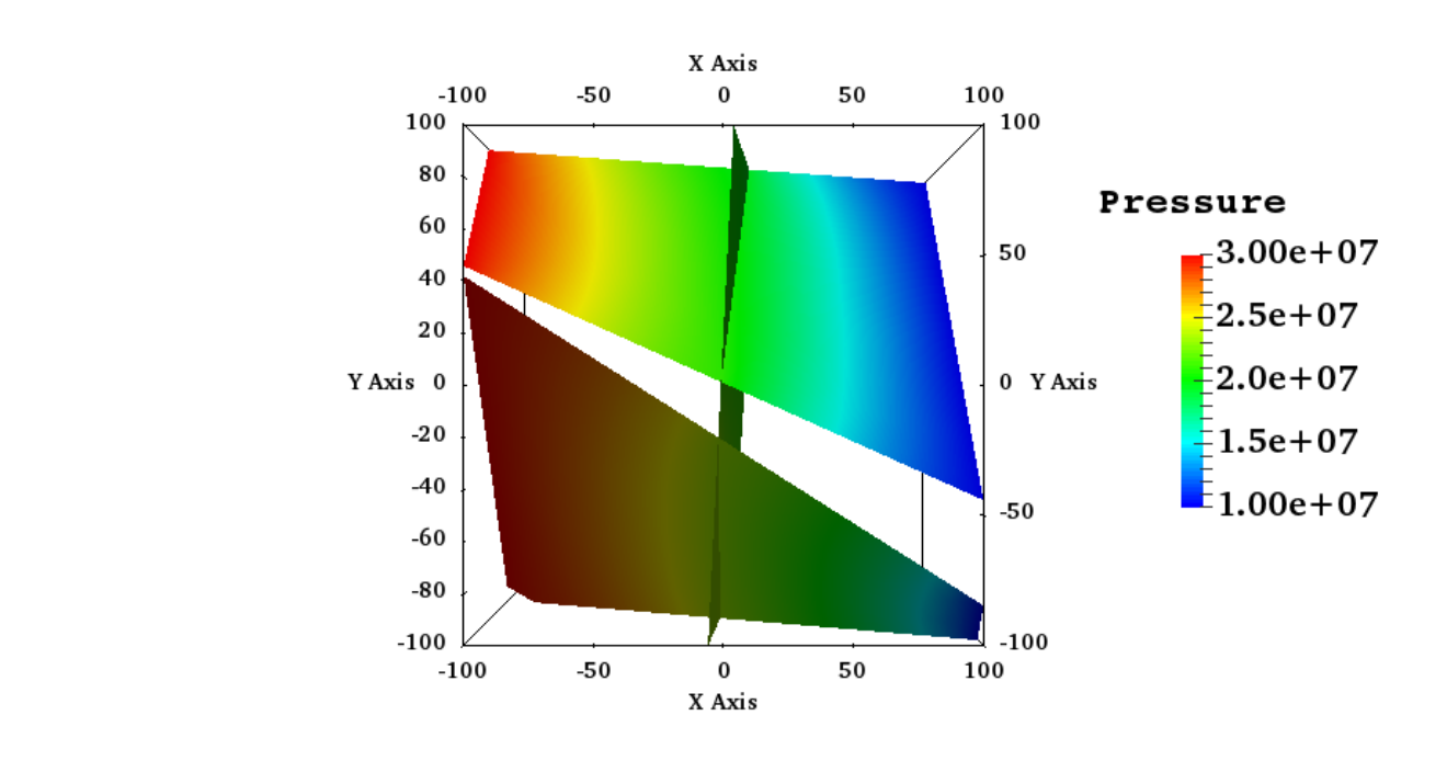
Using these parameters, the fluid pressure profile (which is the true solution) is obtained on the original DFN, shown in Figure 12. Pressure observation data, used in our inversion framework, is sampled at the centroids of the elliptical fractures, whose values are given as follows:
- •
Pressure observation data: MPa, MPa, and MPa.
3.1. Discussion of numerical results and inferences
Using the above observational pressure datasets, inverted seismic events locations and focal mechanisms, we perform sequential inversion analysis to determine the fracture characteristics for various cases discussed in subsection 2.4. The following are the numerical values for the input parameters for Algorithms 1 and 2:
- •
NumCoord = 332, MaxIters = 20, TolValue = , MaxCombo =
- •
The Monte Carlo simulations based on LHS are constructed using the following ranges with NumLHS = 10:
Elliptical fracture lengths (in the direction of minor axis) are chosen to be between 200 m and 300 m. The aspect ratio (major axis length to minor axis length) is varied from 1.0 to 1.5. Based on the case, fracture aperture and permeability ranges are:- Case #1:
-
Log of fracture aperture and log of fracture permeability are varied from -6.0 to -4.0 and -13.0 to -11.0.
- Case #2:
-
Log of mean value of aperture is -5.0 while its standard deviation is varied from 0.6 to 0.9.
- Case #3:
-
and is varied from 0.5 to 2.0
- Case #4:
-
and is varied from 0.5 to 2.0
Remark 3.1.
Numerical simulations are performed on using 32 cores to construct the strike angle and the dip angle discrete probability distributions for the entire seismic events using pure clustering analysis. It should be noted that the total number of possible fracture orientation combinations for 332 seismic events is equal to 6,044,060, which is quite high. To reduce the computational time to calculate the entire discrete probability distribution, we use a combination of Multiprocessing parallelization module and Itertools module in Python. Correspondingly, the computational time for these 6 million combinations is around 904 seconds.
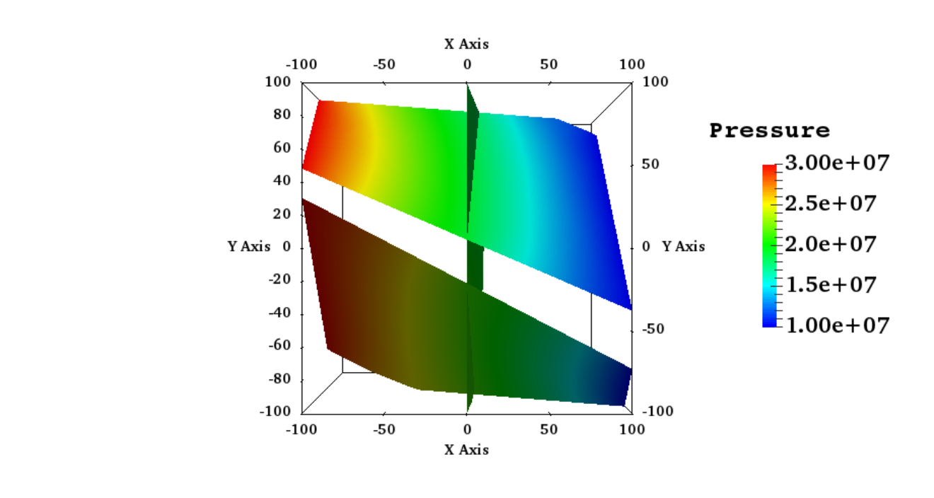
Numerical results are shown in Figures 3–14. From Figures 3–4, the following can be inferred: The strike and dip angles of true fracture planes are close to , , and . From Figures 6–11, which are constructed based on pure clustering analysis of inverted seismic events, a first set of upper and lower bounds on the strike and dip angles can be obtained. However, when used in conjunction with focal mechanisms. These bounds can be further constrained. To crystallize, from Figures 5–11, the following conclusion can be drawn: Based on focal mechanisms of inverted events, discrete probability distributions for strike and dip angles for entire cluster, and discrete probability distributions for strike and dip angles for each of the three different clusters, we have the following hard constraints on the fracture orientation:
- Fracture plane #1:
-
Strike and dip angles vary from and .
- Fracture plane #2:
-
Strike and dip angles vary from and .
- Fracture plane #3:
-
Strike and dip angles vary from and .
Latin hypercube samples are drawn from the above fracture angle ranges and the respective unit normals for fracture planes are obtained. These are provided as inputs for Algorithm 2 to estimate fracture length based on observation data at the observation points. Figure 12 provides the true solution for fluid pressure based on the true set of unit normals for elliptical fractures. Numerical simulations are performed for the four different cases based on the constructed LHS. Figures 13 and 14 provide the contour profiles for fluid pressure for which the misfit functional value is in the order . For Case #3 and Case #4, the parameter is equal to 0.75 and 0.804.
| Case # | Aperture [m] | |||||
|---|---|---|---|---|---|---|
| Frac-1 | Frac-2 | Frac-3 | Frac-1 | Frac-2 | Frac-3 | |
| True value | NA | NA | NA | |||
| 1 | ||||||
| 2 | ||||||
| 3 | ||||||
| 4 | ||||||
| Case # | Permeability | |||||
|---|---|---|---|---|---|---|
| Frac-1 | Frac-2 | Frac-3 | Frac-1 | Frac-2 | Frac-3 | |
| True value | NA | NA | NA | |||
| 1 | ||||||
| 2 | ||||||
| 3 | ||||||
| 4 | ||||||
| Case # | Pressure [MPa] | |||||
|---|---|---|---|---|---|---|
| Frac-1 | Frac-2 | Frac-3 | Frac-1 | Frac-2 | Frac-3 | |
| True value | 21.86 | 19.08 | 18.33 | NA | NA | NA |
| 1 | 21.74 | 19.04 | 18.29 | -0.0054 | -0.0021 | -0.0022 |
| 2 | 21.49 | 19.96 | 18.58 | -0.017 | 0.046 | 0.014 |
| 3 | 22.09 | 19.02 | 18.19 | 0.011 | -0.003 | -0.007 |
| 4 | 21.52 | 18.57 | 17.96 | -0.015 | -0.027 | -0.008 |
| Case # | Axis length [m] | |||||||
|---|---|---|---|---|---|---|---|---|
| Minor (all) | Frac-1 (Major) | Frac-2 (Major) | Frac-3 (Major) | Minor (all) | Frac-1 | Frac-2 | Frac-3 | |
| True value | 250 | 275 | 300 | 312.5 | NA | NA | NA | NA |
| 1 | 245.14 | 255.88 | 255.44 | 263.34 | -0.019 | -0.069 | -0.149 | -0.157 |
| 2 | 280.12 | 335.62 | 301.28 | 338.1 | 0.121 | 0.221 | 0.004 | 0.082 |
| 3 | 245.98 | 296.24 | 300.48 | 306.56 | -0.016 | 0.077 | 0.002 | -0.019 |
| 4 | 250.64 | 272.64 | 289.3 | 303.84 | 0.002 | -0.008 | -0.035 | -0.027 |
A summary of the above parameters are shown in Tables 1, 2, and 4. The following can be inferred based on Figures 3–14 and Tables 1–4:
- Fracture orientation:
-
Pure clustering analysis (statistical approach) without the information from focal mechanisms (physics-based approach) may not always be accurate. But it is the combination of clustering analysis of seismic events and focal mechanisms that can provide reasonably accurate information, thereby ensuring hard constraints on the dominant fracture planes orientation. Details on how we arrived at the fracture angles and number of fracture planes based on a combination of cluster analysis and focal mechanisms are given below:
- •:
- •:
- •:
Strike angle distribution obtained from focal mechanism shows two dominant fracture planes. Dip angle distribution shows three dominant fracture planes.
- •:
Based on the elbow method and focal mechanisms, we can conclude that there are three dominant fracture planes.
- Fracture aperture and permeability:
-
From Table 1, it can inferred that Case #2 has aperture values close to ground truth while Case #4 performs poorly. From Table 2, Case #1 and Case #2 have permeability values close to ground truth while Case #3 and Case #4 deviate considerably. This is due to the nonlinear relationships between fracture aperture and fracture length assumed in these two cases.
- Model pressure values:
- Fracture lengths:
-
From Table 4, the Case #4 has least absolute relative error for minor axis while Case #2 has highest absolute relative error. For major axis, for fracture-1, Case #4 has least error while Case #2 has the highest error. For fracture-2 and fracture-3, Case #3 has the least error while Case #1 has the highest absolute error. In all the cases, the absolute relative error for both major and minor axis are in the order of .
4. CONCLUDING REMARKS
In this paper, we have presented a sequential inversion framework to constrain subsurface fracture network represented as a DFN using geophysical and flow data sets. First, we described the forward models to obtain focal mechanisms and model observation data for flow variables. Second, based on these models we have constructed a novel sequential inversion methodology for various cases to constrain dominant fracture orientation and fracture length. Third, utilizing this framework, we have presented a synthetic numerical example to demonstrate various aspects of the proposed algorithms. From this example, it is apparent that physics-informed clustering analysis, which is a combination of clustering analysis (pure statistical approach) and focal mechanisms (physics-based approach) can provide accurate bounds on the dominant fracture plane orientations. Finally, we discussed various cases to constrain fracture length. From these case studies, it is clear that the model flow data variables are highly dependent on various fracture parameters (which inturn depend on the fracture length in a highly nonlinear fashion). In all these case studies, even though the model observation data is close to the prescribed observation data, there is a wide difference in different fracture parameters. Furthermore, prior analysis on these fracture parameters (such as aperture, transmissivity, and permeability) is needed to better constrain the fracture length.
It is seen from the example problem that the resulting primary variables (such as pressure and flow rate), obtained by solving the governing equations for the flow problem, are very sensitive to the fracture parameters (aperture, transmissivity and its coefficients, and permeability), fracture length, and fracture orientation. Moreover, fracture parameters such as fracture permeability have a nonlinear dependence on the fracture length. This has serious consequences on constraining subsurface DFNs as pressure and flow rate depend on the fracture permeability. Hence, it is a challenge to obtain sharp constraints on the fracture statistics.
The proposed framework and algorithms are general and non-intrusive. They leverage on existing parallel fracture flow simulators to construct bounds on the fracture length and orientation. Moreover, extending the sequential inversion framework proposed in this paper to include various other nearly-orthogonal/complementary datasets (such as chemical, mechanical, and temperature) is straight-forward and requires minimal effort.
Subsequently, in our future works, we will perform detailed sensitivity analysis on these fracture parameters to impose hard/sharp bounds on the fracture length, aperture, transmissivity, and permeability. As the number of fractures increases, more sophisticated methods such as -means clustering, information-theoretic approach, silhouette method, and kernel matrix analysis can be used to determine the number of cluster/fractures [79] rather than relying on traditional elbow method.
APPENDIX
A brief description of the geophysical, subsurface flow, and statistical terminology used in this paper, is given below:
- Discrete Fracture Network (DFN) modeling:
-
The DFN approach is a modeling methodology that seeks to describe the rock mass fracture system in statistical ways by building a series of discrete fracture objects represented as two-dimensional planes in three-dimensional space. The statistics of these networks are based on field observations of fracture properties such as size, orientation and intensity.
- Outcrop:
-
An outcrop is a visible exposure of bedrock or superficial deposits on the surface of the earth.
- Focal mechanism:
-
Seismologists refer to the direction of slip in an earthquake and the orientation of the fault on which it occurs as the focal mechanism. They use the information from seismograms to calculate the focal mechanism.
- Microseismics:
-
In seismology, a microseism is defined as a faint earth tremor caused by natural phenomena. Microseisms are very well detected and measured by means of a broad-band seismograph, and can be recorded anywhere on Earth.
- Shear wave:
-
In seismology, shear waves are one of the two main types of elastic body waves, because they move through the bulk of the object/body under consideration, unlike surface waves.
- Permeability:
-
Permeability in fluid mechanics and the earth sciences is a measure of the ability of a porous material to allow fluids to pass through it.
- Fracture aperture:
-
Fracture aperture is the width of a fracture opening. In quantifying flow through fractures, apertures can be used to calculate permeability by assuming equivalency with flow between two parallel plates.
- Compensated Linear Vector Dipole:
-
The pattern of energy radiation of an earthquake is represented by the moment tensor solution, which is graphically represented by beachball diagrams. An explosive or implosive mechanism produces an isotropic seismic source. Slip on a planar fault surface results in what is known as a double-couple source. Uniform outward motion in a single plane due to normal shortening is known as a compensated linear vector dipole source.
- Geophones:
-
A geophone is a device that converts ground movement (velocity) into voltage, which may be recorded at a recording station. The deviation of this measured voltage from the base line is called the seismic response and is analyzed for structure of the earth.
- Seismic moment:
-
Seismic moment is a quantity used by earthquake seismologists to measure the size of an earthquake. For modern earthquakes, moment is usually estimated from ground motion recordings of earthquakes known as seismograms. For earthquakes that occurred in times before modern instruments were available, moment may be estimated from geologic estimates of the size of the fault rupture and the displacement.
- Green’s function:
-
Green’s function visualizes the effect of source concentrated at a point on different points of the domain. In mathematics, a Green’s function is the impulse response of an inhomogeneous differential equation defined on a domain, with specified initial conditions or boundary conditions. Combining Green’s function with focal mechanism can represent seismic waveforms recorded for a given earthquake.
- -means clustering:
-
Clustering is a process of partitioning a set of data (or objects) into a set of meaningful sub-classes, called clusters. This helps user to understand the natural grouping or structure in a dataset. Clustering is used either as a stand-alone tool to get insight into data distribution or as a pre-processing step for other algorithms. In particular, -means clustering aims to partition observations into clusters in which each observation belongs to the cluster with the nearest mean, serving as a prototype of the cluster [82, 83, 84].
- Latin Hypercube Sampling:
- Sequential geophysical and flow inversion:
-
By this term, we mean that the geophysical data is inverted first. This inversion process results in fracture orientations. Then, we invert for flow data to obtain fracture lengths.
ACKNOWLEDGMENTS
The authors thank U.S. Department of Energy (DOE) SubTER initiative. MKM and SK acknowledge the support of the LANL LDRD Early Career Project 20150693ECR. MKM thanks Hari Viswanathan, Gilles Bussod, and Vamshi Chillara for many useful discussions. MKM also thanks Daniel O’Malley for the help related to MADS software. TC thanks Yu Chen for providing the focal mechanism inversion code.
References
- [1] Rock Fractures and Fluid Flow: Contemporary Understanding and Applications. National Academy Press, Washington D.C., USA, 1996.
- [2] M. K. Mudunuru, S. Kelkar, S. Karra, D. R. Harp, G. D. Guthrie, and H. S. Viswanathan. Reduced-order models to predict thermal output for enhanced geothermal systems. In Proceedings of Stanford Geothermal Workshop, Stanford University, Stanford, CA, USA, 2016.
- [3] M. K. Mudunuru, S. Karra, D. R. Harp, G. D. Guthrie, and H. S. Viswanathan. Regression-based reduced-order models to predict transient thermal output for enhanced geothermal systems. Geothermics, 70:192–205, 2017.
- [4] J. W. Cosgrove and T. Engelder, editors. The Initiation, Propagation, and Arrest of Joints and Other Fractures. Number 231 in Geological Society Special Publication. The Geological Society, London, UK, 2004.
- [5] D. W. Brown, D. V. Duchane, G. Heiken, and V. T. Hriscu. Mining the Earth’s Heat: Hot Dry Rock Geothermal Energy. Springer-Verlag, Berlin, Heidelberg, Germany, 2012.
- [6] R. P. Shaw, editor. Understanding the Micro to Macro Behaviour of Rock-Fluid Systems. Number 249 in Geological Society Special Publication. The Geological Society, London, UK, 2005.
- [7] E. Eberhardt, D. Stead, and T. Morrison, editors. Rock Mechanics: Meeting Society’s Challenges and Demands: Volume-1: Fundamentals, New Technologies, & New Ideas. Taylor & Francis, Boca Raton, Florida, USA, 2007.
- [8] E. Eberhardt, D. Stead, and T. Morrison, editors. Rock Mechanics: Meeting Society’s Challenges and Demands: Volume-2: Case Histories. Taylor & Francis, Boca Raton, Florida, USA, 2007.
- [9] G. H. Spence, J. Redfern, R. Aguilera, T. G. Bevan, J. W. Cosgrove, G. D. Couples, and J.-M. Daniel, editors. Advances in the Study of Fractured Reservoirs. Number 374 in Geological Society Special Publication. The Geological Society, London, UK, 2014.
- [10] F. Zhou, M. Henry, and M. Tombs. Laboratory and field trials of Coriolis mass flow metering for three-phase flow measurement. In Proceedings of International Symposium on Measurement Techniques for Multiphase Flows, volume 1592, pages 105–114, Guangzhou, China, 2014. AIP Publishing LLC.
- [11] S. Kelkar, G. WoldeGabriel, and K. Rehfeldt. Hot Dry Rock Final Report, Geothermal Energy Development at Los Alamos National Laboratory: 1970–1995. Technical Report LA-UR-15-22668, Los Alamos National Laboratory, 2015.
- [12] B. A. Robinson and J. W. Tester. Dispersed fluid flow in fracture reservoir: An analysis of tracer–determined residence time distributions. Journal of Geophysical Research, 89:10374–10384, 1984.
- [13] C. O. Grisby, J. W. Tester, P. E. Trujillo Jr., and D. A. Counce. Rock–Water interactions in the Fenton–Hill, New Mexico, Hot Dry Rock geothermal systems–I. Fluid mixing and chemical geothermometry. Geothermics, 18:629–656, 1989.
- [14] C. O. Grisby, J. W. Tester, P. E. Trujillo Jr., and D. A. Counce. Rock–Water interactions in the Fenton–Hill, New Mexico, Hot Dry Rock geothermal systems–II. Modeling geochemical behavior. Geothermics, 18:657–676, 1989.
- [15] M. Sahimi, M. C. Robertson, and C. G. Sammis. Fractal distribution of earthquake hypocenters and its relation to fault patterns and percolation. Physical Review Letters, 70:2186–2189, 1993.
- [16] A. Roff, W. S. Phillips, and D. W. Brown. Joint structures determined by clustering microearthquakes using waveform amplitude ratios. International Journal for Rock Mechanics and Mining Sciences & Geomechanics Abstracts, 25:627–639, 1996.
- [17] S. N. Pandey, A. Chaudhuri, S. Kelkar, V. R. Sandeep, and H. Rajaram. Investigation of permeability alteration of fractured limestone reservoir due to geothermal heat extraction using three-dimensional Thermo-Hydro-Chemical (THC) model. Geothermics, 51:46–62, 2014.
- [18] S. N. Pandey, A. Chaudhuri H. Rajaram, and S. Kelkar. Fracture transmissivity evolution due to silica dissolution/precipitation during geothermal heat extraction. Geothermics, 57:111–126, 2015.
- [19] M. W. McClure and R. N. Horne. An investigation of simulation mechanisms in enhanced geothermal systems. International Journal of Rock Mechanics & Mining Sciences, 72:242–260, 2014.
- [20] P. K. Kang, Y. Zheng, X. Fang, R. Wojcik, D. McLaughlin, S. Brown, M. C. Fehler, D. R. Burns, and R. Juanes. Sequential approach to joint flow-seismic inversion for improved characterization of fractured media. Water Resources Research, 52:903–919, 2016.
- [21] J. Chen, S. Hubbard, J. Peterson, K. Williams, M. Fienen P. Jardine, and D. Watson. Development of a joint hydrogeophysical inversion approach and application to a contaminated fractured aquifer. Water Resources Research, 42, DOI: 10.1029/2005WR004694, 2006.
- [22] C. Dorn, N. Linde, T. Le Borgne, O. Bour, and M. Klepikova. Inferring transport characteristics in a fractured rock aquifer by combining single-hole ground-penetrating radar reflection monitoring and tracer test data. Water Resources Research, 48, DOI: 10.1029/2011WR011739, 2012.
- [23] J. Geier. Investigation of Discrete-Fracture Network Conceptual Model Uncertainty at Forsmark. Technical report, Swedish Radiation Safety Authority, Stockholm, Sweden, 2011.
- [24] SKB. Long-Term Safety for the Final Repository for Spent Nuclear Fuel at Forsmark. Main Report of the SR-Site Project. Technical Report SKB TR-11-01, Swedish Nuclear Fuel and Waste Management Co., Stockholm, Sweden, 2011.
- [25] L. Hartley and S. Joyce. Approaches and algorithms for groundwater flow modeling in support of site investigations and safety assessment of the Forsmark site, Sweden. Journal of Hydrology, 500:200–216, 2013.
- [26] S. A. Shapiro. Fluid-Induced Seismicity. Cambridge University Press, Cambridge, UK, 2015.
- [27] Induced Seismicity Potential in Energy Technologies. The National Academy Press, Washington D.C, USA, 2012.
- [28] S. Talebi, editor. Seismicity Caused by Mines, Fluid Injections, Reservoirs, and Oil Extraction. Springer-Basel AG, Basel, Switzerland, 1999.
- [29] M. Wyss, K. Shimazaki, and A. Ito, editors. Seismicity Patterns, their Statistical Significance, and Physical Meaning. Birkhäuser-Verlag, Basel, Switzerland, 1999.
- [30] X. E. Refunjol and K. J. Marfurt. Inversion and attribute-assisted hydraulically induced microseismic fracture characterization in the North Texas Barnett Shale. The Leading Edge, 30:292–299, 2011.
- [31] R. J. Michelena, K. S. Godbey, H. Wang, J. R. Gilman, and C. K. Zahm. Estimation of dispersion in orientations of natural fractures from seismic data: Application to DFN modeling and flow simulation. The Leading Edge, 32:1502–1512, 2013.
- [32] S. Dadi, R. Gibson, and K. Wang. Velocity log upscaling based on reversible jump Markov chain Monte Carlo simulated annealing. Geophysics, 81:R293–R305, 2016.
- [33] I. F. Jones, R. I. Bloor, B. L. Biondi, and J. T. Etgen, editors. Prestack Depth Migration and Velocity Model Building, volume 25 of Geophysics Reprint Series. Society of Exploration Geophysicists, Oklahoma, USA, 2008.
- [34] A. Tarantola. Inversion of seismic reflection data in the acoustic approximation. Geophysics, 49:1259–1266, 1984.
- [35] J. Virieux and S. Operto. An overview of full-waveform inversion in exploration geophysics. Geophysics, 74:WCC1–WCC26, 2009.
- [36] F. Waldhauser and W. L. Ellsworth. A double-difference earthquake location algorithm: Method and application to the northern Hayward fault, California. Bulletin of the Seismological Society of America, 90:1353–1368, 2000.
- [37] J. P. Verdon and A. Wüstefeld. Measurement of the normal/tangential fracture compliance ratio (ZN/ZT) during hydraulic fracture stimulation using S-wave splitting data. Geophysical Prospecting, 61:461–475, 2013.
- [38] G. Vlahovic, M. Elkibbi, and J. A. Rial. Shear-wave splitting and reservoir crack characterization: The Coso geothermal field. Journal of Volcanology and Geothermal Research, 120:123–140, 2003.
- [39] K. Srivastava, S. Rani, and D. Srinagesh. A review of -value imaging and fractal dimension studies in the Andaman Sumatra subduction. Natural Hazards, 77:97–107, 2015.
- [40] M. Sahimi. Applications of Percolation Theory. Taylor & Francis, London, UK, 1994.
- [41] M. Sahimi. Flow and Transport in Porous Media and Fractured Rock: From Classical Methods to Modern Approaches. Taylor & Francis, Weinheim, Germany, second, revised and enlarged edition, 2011.
- [42] T. Manzocchi, C. Childs, and J. J. Walsh. Faults and fault properties in hydrocarbon flow models. Geofluids, 10:94–113, 2010.
- [43] B. Berkowitz. Characterizing flow and transport in fractured geological media: A review. Advances in Water Resources, 25:861–884, 2002.
- [44] C. K. Morley and C. W. Nixon. Topological characteristics of simple and complex normal fault networks. Journal of Structural Geology, 84:68–84, 2016.
- [45] C. K. Morley and C. W. Nixon. Fractures, faults, and hydrocarbon entrapment, migration and flow. Marine and Petroleum Geology, 17:797–814, 2000.
- [46] L. Moreno and I. Neretnieks. Fluid flow and solute transport in a network of channels. Journal of Contaminant Hydrology, 14:163–192, 1993.
- [47] P. K. Kang, T. Le Borgne, M. Dentz, O. Bour, and R. Juanes. Impact of velocity correlation and distribution on transport in fractured media: Field evidence and theoretical model. Water Resources Research, 51:940–959, 2015.
- [48] J. Hofrichter and G. Winkler. Statistical analysis for the hydrogeological evaluation of the fracture networks in hard rocks. Environmental Geology, 49:821–827, 2006.
- [49] G. Beardsmore. Data fusion and machine learning for geothermal target exploration and characterization. Technical report, National ICT Australia Limited (NICTA), Australia, 2014.
- [50] A. Ghassemi. A review of some rock mechanics issues in geothermal reservoir development. Geotechnical and Geological Engineering, 30:647–664, 2012.
- [51] J. Ziagos, B. R. Phillips, A. Jelacic, G. Stillman, and E. Hass. A technology roadmap for strategic development of enhanced geothermal systems. In Proceedings of Stanford Geothermal Workshop, Stanford University, Stanford, CA, USA, 2013.
- [52] J. D. Hyman, C. W. Gable, S. L. Painter, and N. Makedonska. Conforming Delaunay triangulation of stochastically generated three dimensional discrete fracture networks: A feature rejection algorithm for meshing strategy. SIAM Journal on Scientific Computing, 36:A1871–A1894, 2014.
- [53] J. D. Hyman, S. Karra, N. Makedonska, C. W. Gable, S. L. Painter, and H. S. Viswanathan. DFNWORKS: A discrete fracture network framework for modeling subsurface flow and transport. Computers & Geosciences, 84:10–19, 2015.
- [54] N. Makedonska, S. L. Painter, Q. M. Bui, C. W. Gable, and S. Karra. Particle tracking approach for transport in three-dimensional discrete fracture networks. Computers & Geosciences, 19:1123–1137, 2015.
- [55] S. Karra, N. Makedonska, H. S. Viswanathan, S. L. Painter, and J. D. Hyman. Effect of advective flow in fractures and matrix diffusion on natural gas production. Water Resources Research, 51:8646–8657, 2015.
- [56] J. D. Hyman, S. L. Painter, H. S. Viswanathan, N. Makedonska, and S. Karra. Influence of injection mode on transport properties in kilometer-scale three-dimensional discrete fracture networks. Water Resources Research, 51:7289–7308, 2015.
- [57] MADS: Model Analysis & Decision Support. URL: http://mads.lanl.gov/; http://madsjulia.lanl.gov/.
- [58] K. Aki and P. C. Richards. Quantitative Seismology. University Science Books, California, USA, second edition, 2002.
- [59] C. Chapman. Fundamentals of Seismic Wave Propogation. Cambridge University Press, Cambridge, UK, 2004.
- [60] P. M. Shearer. Introduction to Seismology. Cambridge University Press, New York, USA, second edition, 2009.
- [61] H. Sato, M. C. Fehler, and T. Maeda. Seismic Wave Propogation and Scattering in the Heterogeneous Earth. Springer, Berlin, Heidelberg, second edition, 2012.
- [62] Y. Chen, L. Wen, and C. Ji. A cascading failure during the 24 May 2013 great Okhotsk deep earthquake. Journal of Geophysical Research: Solid Earth, 119:3035–3049, 2014.
- [63] G. F. Pinder and M. A. Celia. Subsurface Hydrology. John Wiley & Sons, Inc., New Jersey, USA, 2006.
- [64] P. C. Lichtner, G. E. Hammond, C. Lu, S. Karra, G. Bisht, B. Andre, R. T. Mills, and J. Kumar. PFLOTRAN User Manual: A Massively Parallel Reactive Flow and Transport Model for Describing Surface and Subsurface Processes. Technical Report LA-UR-15-20403, Los Alamos National Laboratory, 2015.
- [65] T. Okada, T. Matsuzawa, N. Umino, K. Yoshida, A. Hasegawa, H. Takahashi, T. Yamada, M. Kosuga, T. Takeda, A. Kato, T. Igarashi, K. Obara, S. Sakai, A. Saiga, T. Iidaka, T. Iwasaki, N. Hirata, N. Tsumura, Y. Yamanaka, T. Terakawa, H. Nakamichi, T. Okuda, S. Horikawa, H. Katao, T. Miura, A. Kubo, T. Matsushima, K. Goto, and H. Miyamachi. Hypocenter migration and crustal seismic velocity distribution observed for the inland earthquake swarms induced by the 2011 Tohoku-Oki earthquake in NE Japan: Implications for crustal fluid distribution and crustal permeability. Geofluids, 15:293–309, 2015.
- [66] H. L. Vacher. Computational Geology 12 – Cramer’s Rule and the Three-Point Problem. Journal of Geoscience Education, 48:522–531, 2000.
- [67] B. S. Everitt, S. Landau, M. Leese, and D. Stahl. Cluster Analysis. Wiley Series in Probability and Statistics. John Wiley & Sons, Ltd.,, West Sussex, UK, fifth edition, 2011.
- [68] E. Jones, T. Oliphant, P. Peterson, et al. Scipy: Open Source Scientific Tools for Python. URL: http://www.scipy.org/.
- [69] Multiprocessing: Process-based “threading" interface in Python. URL: https://docs.python.org/2/library/multiprocessing.html.
- [70] S. A. Flewelling, M. P. Tymchak, and N. Warpinski. Hydraulic fracture height limits and fault interactions in tight oil and gas formations. Geophysical Research Letters, 40:3602–3606, 2013.
- [71] P. M. Adler, J.-F. Thovert, and V. V. Mourzenko. Fractured Porous Media. Oxford University Press, Oxford, UK, 2013.
- [72] G. W. Milligan and M. C. Cooper. An examination of procedures for determining the number of clusters in a data set. Psychometrika, 50:159–179, 1985.
- [73] C. A. Sugar and G. M. James. Finding the number of clusters in a dataset: An information-theoretic approach. Journal of the American Statistical Association, 98:750–763, 2003.
- [74] M. Yan and K. Ye. Determining the number of clusters using the weighted gap statistic. Biometrics, 63:1031–1037, 2007.
- [75] Z. He, A. Cichocki, S. Xie, and K. Choi. Detecting the number of clusters in -way probabilistic clustering. IEEE Transactions on Pattern Analysis and Machine Intelligence, 32:2006–2021, 2010.
- [76] J. Wang. Consistent selection of the number of clusters via cross-validation. Biometrika, pages 893–904, 2010.
- [77] R. L. Thorndike. Who belongs in the family? Psychometrika, 18:267–276, 1953.
- [78] M. M. T. Chiang and B. Mirkin. Intelligent choice of the number of clusters in -means clustering: An experimental study with different cluster spreads. Journal of Classification, 27:3–40, 2010.
- [79] T. M. Kodinariya and P. R. Makwana. Review on determining number of cluster in -means clustering. International Journal, 6:90–95, 2013.
- [80] R. Tibshirani and G. Walther. Cluster validation by prediction strength. Journal of Computational and Graphical Statistics, 14:511–528, 2005.
- [81] R. Tibshirani, G. Walther, and T. Hastie. Estimating the number of clusters in a data set via the gap statistic. Journal of the Royal Statistical Society: Series B (Statistical Methodology), 63:411–423, 2001.
- [82] T. Kanungo, M. D. Mount, N. S. Netanyahu, C. D. Piatko, R. Silverman, and A. Y. Wu. An efficient -means clustering algorithm: Analysis and implementation. IEEE Transactions on Pattern Analysis and Machine Intelligence, 24:881–892, 2002.
- [83] M. C. Setodji and R. D. Cook. -means inverse regression. Technometrics, 46:421–429, 2004.
- [84] A. K. Jain. Data clustering: 50 years beyond -means. Pattern Recognition Letters, 31:651–666, 2010.
- [85] M. D. McKay, R. J. Beckman, and W. J. Conover. Comparison of three methods for selecting values of input variables in the analysis of output from a computer code. Technometrics, 21:239–245, 1979.
- [86] R. J. McKay. The adequacy of variable subsets in multivariate regression. Technometrics, 21:475–479, 1979.
- [87] W. Dzwinel, D. A. Yuen, K. Boryczko, Y.-B. Zion, S. Yoshioka, and T. Ito. Cluster analysis, data-mining, multi-dimensional visualization of earthquakes over space, time and feature space. Nonlinear Processes in Geophysics, 12:117–128, 2005.
- [88] I. Zaliapin, A. Gabrielov, V.-K. Borok, and H. Wong. Clustering analysis of seismicity and aftershock identification. Physical Review Letters, 101:018501(4), 2008.