Theoretical description of circular dichroism in photoelectron angular distributions of randomly oriented chiral molecules after multi-photon photoionization
Abstract
Photoelectron circular dichroism refers to the forward/backward asymmetry in the photoelectron angular distribution with respect to the propagation axis of circularly polarized light. It has recently been demonstrated in femtosecond multi-photon photoionization experiments with randomly oriented camphor and fenchone molecules [C. Lux et al., Angew. Chem. Int. Ed. 51, 5001 (2012); C. S. Lehmann et al., J. Chem. Phys. 139, 234307 (2013)]. A theoretical framework describing this process as (2+1) resonantly enhanced multi-photon ionization is constructed, which consists of two-photon photoselection from randomly oriented molecules and successive one-photon ionisation of the photoselected molecules. It combines perturbation theory for the light-matter interaction with ab initio calculations for the two-photon absorption and a single-center expansion of the photoelectron wavefunction in terms of hydrogenic continuum functions. It is verified that the model correctly reproduces the basic symmetry behavior expected under exchange of handedness and light helicity. When applied it to fenchone and camphor, semi-quantitative agreement with the experimental data is found, for which a sufficient wave character of the electronically excited intermediate state is crucial.
Keywords:
photoelectron angular distributions, circular dichroism, irreducible tensor fields, Wigner rotation matrices, Wigner symbolsI Introduction
Photoelectron spectroscopy is a powerful tool for studying photoionization dynamics. Intense short laser pulses for the ionization, which easily drive multi-photon transitions, allow to observe effects in table-top experiments that otherwise would require synchrotron radiation. A recent example is the photoelectron circular dichroism (PECD) of chiral molecules [1, 2, 3, 4, 5]. It refers to the forward/backward asymmetry with respect to the light propagation axis in the photoelectron angular distribution (PAD) obtained after excitation with circularly polarized light [6, 7, 8]. When the PAD is expanded in Legendre polynomials, a PECD is characterized by the expansion coefficients of the odd-order polynomials with the highest order polynomial being determined by the order of the process, i.e., the number of absorbed photons [6, 9].
A theoretical description of such experiments with intense femtosecond laser pulses requires proper account of the multi-photon excitation pathways. In the pioneering work of McClain and co-workers [10, 11, 12, 13], a model for the simultaneous absorption of two photons including the corresponding modified molecular selection rules was formulated. Two-photon circular dichroism was developed in Ref. [14], attributing the effect to a difference in the absorption coefficient for the two left and two right polarized photons. These approaches are based on a perturbation expansion of the light-matter interaction. The strong-field approximation provides an alternative description which is particularly suited for very intense fields [15, 16].
Multi-photon transitions driven by strong femtosecond laser pulses may or may not involve intermediate states.
In recent experiments with bicyclic ketones [1, 2, 3, 4, 5], a 2+1-REMPI process was employed. The nature of the intermediate state remains yet to be clarified. A first theoretical study used the strong-field approximation [17]. While the standard strong-field approximation using a plane wave basis for the photoelectron was found to fail in describing PECD, accounting for the Coulomb interaction between photoelectron and photoion in the Born approximation allowed for observation of PECD. However, the PAD did not agree with the epxerimental ones. This may be explained by the role fo the intermediate state in the REMPI process which necessarily is ignored in the strong-field approximation [17].
Here, we take the opposite approach, starting with a perturbation theory treatment of the multi-photon process. Thus, ionization is viewed as a (weak) one-photon transition into the continuum, the ’initial’ state of which is prepared by non-resonant two-photon absorption. Such an approach is motivated by the moderate intensities, of the order of W/cm2, used in the experiments [1, 2, 3, 4, 5]. Although clearly in the multi-photon regime, such intensities can be described comparatively well by low order perturbation theory [18, 19, 20].
The non-resonant two-photon preparation step yields an important difference compared to pure one-photon excitation [21]. In the latter case, the first order Legendre polynomial alone accounts for the PECD [22, 23, 24]. This results from the random orientation of the molecules, or, in more technical terms, from integrating the differential cross section over the Euler angles. In contrast, non-resonant two-photon excitation may lead to an orientation-dependent probability distribution of the molecules in the resonant intermediate state [2]. In this case, the maximum order of Legendre polynomials contributing to the PAD is not limited to 2, but 6 for a 2+1 process. Whether the two-photon absorption is orientation-dependent is determined by the two-photon transition matrix elements. Here, we calculate the two-photon transition matrix elements using state of the art ab initio methods. However, for molecules as complex as camphor and fenchone, it is extremely challenging to model the complete photoionization process from first principles, even when using the most advanced ab initio methods. We therefore split the theoretical description into two parts.
As long as all electrons remain bound, state of the art quantum chemical approaches, for example the coupled cluster methods, can be used to accurately determine the electronic wave functions. However, once an electron starts to leave the ionic core, the standard basis sets of electronic structure theory are not well adapted. An alternative is offered by a single-center expansion into eigenfunctions of a hydrogen-like atom for which both bound and continuum functions are known analytically. The hydrogenic continuum functions properly account for the long-range Coulomb interaction between ionic core and ejected electron but neglect the effect of short-range correlations in the ionization step. The basis functions for the single center expansion are chosen such as to yield the simplest possible model that is able to reproduce the laboratory-frame photoelectron angular distributions (LF-PADs) resulting from a 2+1-REMPI process in randomly oriented chiral molecules. The two descriptions are matched at the resonant, electronically excited intermediate state by projecting the numerically calculated wavefunction onto the basis functions of the single center expansion.
Our approach of calculating the PAD as a one-photon absorption cross section for an effective “initial” state in a single center expansion, while neglecting dynamical effects, allows us to generalize our findings to chiral molecules other than fenchone or camphore. In particular, we analyze the role of the laser polarization for each step in the 2+1 ionization process and determine the conditions on the two-photon absorption matrix elements for yielding PECD.
The remainder of the paper is organized as follows: Our theoretical framework is introduced in Sec. II. In detail, Sec. II.1 defines the PAD as one-photon photoionization cross section and summarizes the single center expansion. To make connection with experiment, the cross sections need to be transformed from the molecule-fixed frame into the laboratory frame and averaged over the random orientations of the molecules. The corresponding expressions for a 2+1 REMPI process are presented in Sec. II.2 with the details of the derivation given in the appendix. The symmetry properties required for observing PECD are analyzed in Sec. II.3. Section III is dedicated to ab initio calculations for the intermediate, electronically excited states and the two-photon absorption matrix elements. Section III.1 presents the computational details and Sec. III.2 the results. The one-center reexpansion required for matching the numerical results to the single-center description derived in Sec. II is described in Sec. III.3. Our numerical results for the PAD of camphor and fenchone and the corresponding PECD are presented in Sec. IV with Sec. IV.1 dedicated to fenchone and Sec. IV.2 to camphore. Our findings are summarized and discussed in Sec. IV.3. Section V concludes.
II Model
We model the resonantly enhanced multi-photon photoionization as a 2+1 process, assuming the last photon to constitute a weak probe of the molecular state that is prepared by non-resonant two-photon absorption. For simplicity, we employ the strict electric dipole approximation. That is, contributions from magnetic dipole terms, which are important for circular polarization dependent differences in absorption cross sections, and higher order electric and magnetic multipole terms are neglected.
Defining two coordinates systems, the molecular frame of reference and the laboratory frame , denotes the polarization of the laser field with respect to the laboratory frame (where we distinguish the polarization of the ionizing photon, from that of the first two photons, ). For convenience, we work in the spherical basis. Thus, and correspond to the spherical unit vectors in the laboratory frame, with denoting left/right circular and linear polarization of the laser beam which propagates in the positive direction (the relation between the spherical and Cartesian unit vectors is found in Eq. (A.3)). Primed (unprimed) coordinates refer the laboratory (molecular) frame of reference throughout. Both frames, and , are related by an arbitrary coordinate rotation , where denote the Euler angles defining the orientation of with respect to .
Consider a one-photon () transition in a molecule whose orientation with respect to is given by the Euler angles . The corresponding differential photoionization cross section, when measured in the molecular frame , reads, within perturbation theory and the electric dipole approximation and in SI units [25],
| (1) |
where with being the fine-structure constant, the energy of the ionizing photon, the reduced Planck constant and the position operator of the electron (or a sum of the various position operators in the multi-electron case). The polarization of the electric field in the laboratory frame of reference is specified by , where takes the value 0 for linear and for left (right) circular polarization, respectively. denotes an energy normalized molecular state with one electron transfered to the ionisation continuum with asymptotic electron linear momentum . is the (bound, unity normalized) molecular state prepared by the non-resonant two-photon absorption, which is defined in the molecular frame of reference. In Eq. (1), we employ the standard notation for doubly differential cross sections in the molecular frame of reference [24, 26, 27] that depend not only on the solid angle but also on the orientation of the molecule via the Euler angles . We utilize a single-center approximation [28] which allows us to calculate the matrix elements in Eq. (1) explicitly. That is, we project the multi-electron wave function obtained from ab initio calculations, , on one-electron basis functions and neglect electron correlations in the continuum description. We first discuss in Sec. II.1 our choice of and then explain below in Sec. II.2 how to connect the differential ionization cross section to the experimentally measured photoelectron angular distributions.
II.1 Single center expansion
The “initial” state for the one-photon ionization is a multi-electron wavefunction which is usually expanded in specially adapted basis functions developed in quantum chemistry. In contrast, the single center expansion is based on the fact that any molecular wavefunction can be written as a linear combination of functions about a single arbitrary point [28]. Of course, such an ansatz will converge very slowly, if the multi-center character of the wavefunction is important. Writing the wavefunction of the electronically excited state of the neutral molecule, that is prepared by the two-photon absorption process, as , we expand it into eigenfunctions of a hydrogen-like atom,
| (2) |
Here, stands for the unknown expansion coefficients, denotes the radial eigenfunctions of the hydrogen-like atom, and are the spherical harmonics. refers to the polar and azimuthal angles of the position vector in the molecular frame of reference. Note that all information about the geometry and the symmetry properties of the “initial” electronically excited state is contained in the expansion coefficients . The number of basis functions must be truncated in any actual calculation, i.e.,
| (3) |
Strictly speaking, all molecular orbitals that are involved in Slater determinants describing the excited state should be subject to the single center expansion. In the present model, we employ an effective one-electron picture by expanding only one representative virtual orbital around the single center, namely the one that is additionally occupied in the supposedly leading configuration for the respective excited state.
We will also ask what the simplest possible model is that gives rise to PECD. In this case, we assume a single quantum number , , to contribute to Eq. (2), i.e.,
| (4) |
where refers to the highest angular momentum state appearing in the “initial” wavefunction. It follows from basic symmetry arguments that the minimal value of for which a PECD can be expected is , that is, at least -orbitals are required.
We model the photoionization as a one-electron process arising from a hydrogenic-like system exclusively, which allows for neglecting the bound molecular part (the remaining molecular parent ion) in . Thus, the resulting continuum wave functions, , are expanded into partial waves in a way that allows for an explicit expression of the photoionization cross section in terms of the scattering solid angle [29, 27, 30, 23],
| (5) |
Here, and correspond to the spherical harmonics describing the orientation of the photoelectron position and momentum, respectively, and is the radial part of the photoelectron wavefunction. For simplicity, we use here and in the following as an abbreviation for . Modeling photoionization as a one-electron process, we can approximate
| (6) |
where are the well-known radial continuum wavefunctions of the hydrogen atom, recalled in Appendix A.1, and stands for the Coulomb phase shift of the th scattered partial wave, with [27, 24, 30]. Note that we expect the phase shift for molecules to depend on and since the molecular potential of chiral molecules is not spherically symmetric. Neglecting the -dependence of the phase shift involves no approximation when using Eq. (2) since the hydrogen eigenfunctions form a complete orthonormal basis. However, this is not true anymore when truncating the basis, cf. Eq. (3). Our ansatz thus involves an additional approximation, namely Eq. (6).
By construction, Eq. (6) yields orthogonality between bound and unbound wavefunctions which is required to avoid spurious singularities [29] and reproduce the correct threshold behavior of the photoioization cross-sections [31]. With the approximation of Eq. (6), we account for the long-range Coulomb interaction between photoelectron and a point charge representing the ionic core but neglect the short-range static exchange. Also, dynamic changes in the electron distribution, such as adjustments of the electronic cloud due to nuclear motion, as well as the interaction of the outgoing photoelectron with the driving electric field upon photoionization are neglected.
Inserting Eq. (6) into Eq. (5) yields
| (7) |
and we can evaluate the matrix element in Eq. (1). Because the wavefunctions are given in the molecular frame of reference, we need to rotate the spherical unit vector in Eq. (1) into that frame [24]. Expanding the rotation operator connecting and into irreducible rank 1 tensor representations, cf. Appendix A.3, Eq. (1) becomes
| (8) | |||||
Inserting Eqs. (4) and (7) to evaluate the overlap integrals yields
| (9) | |||||
In Eq. (9), we have introduced radial and angular integrals and , given by
| (10a) | |||||
| for a fixed in Eq. (2) with , and | |||||
| (10b) | |||||
with
and using Wigner symbols [32, 33, 34, 35]. The angular integral determines, for each spherical unit vector , the selection rules between the angular components of the bound exited electronic state with quantum numbers , and the partial wave components of the continuum wavefunction with quantum numbers , . Equation (10b) implies that transitions are allowed if and only if is even and for all . This is a special case of the more general rule for multipole transitions derived in Ref. [9]. The angular integrals can be evaluated analytically using the standard angular momentum algebra, whereas the radial integrals in Eq. (10a) are computed numerically.
The choice of basis to describe the radial part of the continuum wavefunction determines the weight with which each excited state expansion coefficient contributes to the PAD, cf. Eqs. (9) and (10a). Thus, choosing for example planes waves, i.e., the eigenfunctions of the “free” photoelectron, which is described in terms of the Bessel functions [32, 33, 35], and does not take into account the Coulomb interaction between the outgoing photoelectron and the remaining ion, would translate into a PAD different from the one obtained with the hydrogenic continuum wavefunctions of Eq. (7). Whether or not the model is able to reproduce the measured Legendre coefficients will to some extent depend on the choice of basis for the radial part in Eq. (5).
The missing ingredient to determine the differential photoionization cross section, Eq. (1), are the expansion coefficients, , of the intermediate excited state wavefunction. They can either be used as fitting parameters or determined from ab initio calculations, see Sec. III .
Two more steps are then required to connect the differential ionization cross section to the experimentally measured PAD. First, the PAD is measured in the laboratory frame and the differential ionization cross section thus needs to be rotated from the molecular into the laboratory frame. Second, the orientation of the molecule with respect to the laboratory frame, defined by the polarization axis of the laser electric field, is arbitrary. We therefore need to average over all possible orientations, i.e., integrate over the Euler angles , , , as we consider a randomly oriented initial ensemble of molecules.
II.2 Photoelectron Angular Distributions
Rotating the differential cross section from the molecular into the laboratory frame requires rotation of the continuum state into using the inverse of Eq. (49). This leads to
| (11) | |||||
where is defined in Eq. (69) in Appendix B.1. denotes the associate Legendre polynomials. A detailed derivation of Eq. (11) is found in Appendix B.1.
When averaging over all orientations in the second step, we need to account for the fact that the probability for non-resonant two-photon absorption from the ground state to the intermediate electronically excited state is, depending on the properties of the two-photon absorption tensor, not isotropic. The differential ionization cross section in the laboratory frame therefore needs to be weighted by the probability of the electronically excited state to be occupied after absorption of the first two (identical) photons. Thus, the cross section for photoemission into a solid angle around the axis in the laboratory frame, after one-photon transition from the electronically excited intermediate state, is given by
| (12) |
where denotes the orientation-dependent probability to reach the intermediate excited state by absorption of two identical photons from the ground state. Equation (12) assumes a molecule to have, in its electronic ground state, an initial orientation of with respect to the laboratory frame of reference. Note that Eq. (12) makes an additional assumption, namely the relative phase between the two-photon and one-photon steps to be irrelevant for the photoelectron spectrum and angular distribution. For a discussion of similar approximations in related multiphoton transitions between bound states, see for instance Refs. [12, 11].
The experimentally measured PAD contains contributions from all molecules in the sample, each of them with a specific orientation . The total photoelectron signal is therefore obtained by an incoherent summation over the contributions from all molecules. This is equivalent to integrating Eq. (12) over the Euler angles weighted by the probability of two-photon absorption. The “averaged” photoionization cross section in the laboratory frame therefore reads,
| (13) |
where the integration is carried over the Euler angles .
The orientation-dependent probability to reach the intermediate excited state, , is obtained from the transition probability for two-photon absorption from the ground state to the intermediate electronically excited state . The latter in general is defined as [36]
| (14a) | |||||
| where , in the strict electric dipole approximation, , reads | |||||
| (14b) | |||||
| In Eq. (14b), denotes the polarization direction (without specifying a certain frame of reference) of photon () with energy . | |||||
To shorten notation, the polarization independent quantity in Eq. (14a) contains all prefactors,
with being the elementary charge, and where and refer to the incident laser-photon-flux (of type ) and the energy flux per unity frequency (of type ), respectively [36]. Evaluation of Eq. (14b) requires a frame transformation, since the wavefunctions involved in the two-photon transition matrices are known in the molecular frame whereas the polarization directions of the photons are given in the laboratory frame of reference. As before, transformation of the polarization directions from the laboratory frame to the molecular frame is carried out by means of the Wigner rotation matrices around the Euler angles . Consequently, the orientation dependent two-photon absorption probability is obtained as
| where we have applied the properties of the rotation matrices between both frames, detailed in Appendix A.3, to Eq. (14b). In Eq. (), denotes the two-photon absorption tensor in the molecular frame of reference, whose tensor elements reads, | |||||
In Eq. (), denotes the polarization direction in the laboratory frame of reference, i.e. , driving the two-photon absorption process, both photons having the same polarization direction. Additionally, the indexes and take the values . Finally, denotes the spherical component of the position operator , with . The correspondence between the spherical and Cartesian components of are detailed in Eq. (A.3). Hence, it is straightforward to write in terms of the tensor elements written in the Cartesian basis, , for , cf. Eq. (104). The correspondences are detailed in Eq. (A.3), in Appendix A.3.
A further step consist of normalizing the probability density, such that the normalization condition,
| (16) |
is fulfilled. Using the properties of addition of angular momenta, it is straightforward to find that the normalization factor reads, upon integration of Eq. () over the Euler angles,
| (17a) | |||||
| where we have defined, | |||||
with . To retrieve Eqs. (17), we have made use of the properties involving the product of two Wigner rotations matrices, as well as the integration involving a product of three Wigner rotations matrices, and apply them to Eq. (). These properties are outlined in Eq. (63) and Eq. (80), in in Appendix A.3 and Appendix B.3, respectively.
Finally, the orientation dependent probability density reads,
| (18) |
with . In order to alleviate notations, and unless otherwise stated, we write . It is important to note, however, that in practice, computation of is not required, since this factor is common to all Legendre coefficients, and all of them are given, as in the experiment [1, 4], normalized with respect to .
Each component of the second-rank tensor determines a property of the system, namely, the average transition rate. As a result of that the tensor has two types of symmetry properties. The first one is due to an intrinsic symmetry originated from the property itself. For instance, defines the probability of a absorption of two identical photons. Since two photons of the same energy and polarization are not the same, has to be symmetric. The second type of symmetry comes from the geometric symmetry of the molecule, and that specifies which of tensor components have to be zero [37, 38].
In the isotropic case, , and evaluation of Eq. (13) is analogous to integrating over Eq. (11), resulting in the standard expressions for the differential photoionization cross section [22, 24, 29, 23, 39, 3]: If the weak probe photon is linearly polarized (), only and can become non-zero, whereas for circularly polarized light, , and can have non-vanishing values. Moreover, the laboratory frame PAD preserves the cylindrical symmetry with respect to the propagation direction of the light , i.e., in Eq. (11).
The situation changes if the probability to populate the intermediate electronically excited state becomes anisotropic. If this probability depends on the initial orientation of the molecule, given in terms of the Euler angles with respect to the laboratory frame , the Wigner rotation matrices in Eq. () couple to those in Eq. (11). Upon integration over the Euler angles in Eq. (13), this gives rise to higher order Legendre polynomials in the PAD, as we show now. To evaluate the angular momentum coupling in Eq. (13), we expand the norm squared in Eq. (). Making use of the product rule for Wigner rotation matrices, Eq. () then becomes
| (19a) | |||||
| with , and where we have defined | |||||
| (19b) | |||||
with . In Eq. (19a), the orientation dependence is contained in , the polarisation dependence in and the dependence on molecular parameters in . The derivation of Eqs. (19), employing the standard angular momentum algebra, is presented in Appendix B.2. We make once more use of the product rule for two rotation matrices, namely those involving the laser polarization in Eq. (11), cf. Eq. (63) in Appendix B.3. Thus, a product of three rotation matrices is obtained when inserting Eqs. (19) and (76), into Eq. (12). Evaluating the products of the Wigner symbols, the differential cross section, Eq. (12), for a specific orientation of the molecule becomes
| (20a) | |||||
| where the only orientation-dependent quantity, , is given by | |||||
| (20b) | |||||
Note that the summation in Eq. (20b) runs over all indices, except and , i.e., , with and appearing from the coupling of the first and second Wigner rotation matrices in Eq. (11), c.f. Eq. (75). The specific form of is detailed in Eq. (79), in Appendix B.3.
We can now use the integral properties of a product of three Wigner rotation matrices [35, 33, 32], c.f. Eq. (80) in Appendix B.3. Integration of over the Euler angles then yields
| (21) | |||||
Note that the second Wigner symbol in the right-hand side of Eq. (21) is non-zero only if and is even with . Because , the terms depending on the azimuthal angle in Eq. (11) do not contribute and we retrieve cylindrical symmetry for the PAD of Eq. (13) which can thus be expressed in terms of Legendre polynomials. Furthermore, according to the fifth and sixth Wigner symbols in Eq. (19b), because , and according to the first and second Wigner symbols in Eq. (19b). The same applies to , reflecting the addition of angular momentum in a two-photon absorption process.
Making use, in Eq. (21), of the fact that the non-zero contributions for are given by , c.f. Eq. (75), one obtains that runs from to , and higher orders give only vanishing contributions. Therefore, the highest order Legendre polynomial that contributes to the PAD is , as expected for a 2+1 process from the rule [22].
Finally, evaluating Eq. (13) with the help of Eq. (21) yields the experimentally measured PAD that is obtained for an initial ensemble of randomly oriented molecules,
| (22a) | |||||
| with coefficients | |||||
| (22b) | |||||
with , and . Derivation of Eq. (22) is explicitly detailed in Appendix B.3. Note that the coefficients depend on the expansion coefficients describing the intermediate electronically exited state, the two-photon absorption tensor elements, , and the laser polarization directions of the two-photon absorption step, , and of the one-photon ionization, .
We would like to emphasize that the contribution of Legendre polynomials with order higher than 2 in Eq. (22) is due to the orientation dependence of populating the intermediate electronically excited state by two-photon absorption from the electronic ground state. That is, the density expresses the fact that molecules with a certain orientation have a larger probability to undergo non-resonant two-photon absorption than molecules with some other orientation . So although the molecules are assumed to be completely randomly oriented with respect to the laser beam axis when they are in their electronic ground state, an effective alignment results for those molecules that absorb two photons. This effective alignment results from selection of certain orientations rather than rotational dynamics which would occur on a much slower timescale. The contribution of higher order Legendre polynomials to the PAD is then entirely determined by the properties of the two-photon absorption tensor and the electronically excited state. In order to interpret the experimentally observed PADs for fenchone and camphor in terms of their expansion in Legendre polynomials, at least qualitatively, we estimate and using ab initio calculations or via fitting. Before presenting the corresponding details in Sec. III, we discuss below the basic symmetry properties of these parameters of our model as well as the dependence on the laser polarization directions , .
II.3 PECD and symmetry
By definition, PECD is obtained if the sign of the odd Legendre coefficients change when the helicity of the electric field changes. Analogously, for fixed electric field helicity, the odd Legendre coefficients change sign when enantiomers are interchanged. We therefore first inspect sign changes in the Legendre coefficients for molecules of opposite handedness within our one-center expansion framework. The relation between a given enantiomer and its mirror image is given by the parity operator, which changes the coordinates to . We therefore check, in the following, that our model transforms properly under parity.
Moreover, we determine the role that the excited state coefficients and two-photon absorption tensor elements play for each Legendre coefficient that contributes to the PAD. To this end, we rewrite Eq. (22b), expressing each explicitly in terms of the and ,
Equation (II.3) allows for determining each Legendre coefficient as a function of the intermediate electronically excited state via and , i.e., it connects the measured Legendre coefficients to the electronic structure properties. We can thus compare the contribution of different to different Legendre coefficients , and explain differences, observed e.g. for different molecules, in terms of the electronic structure. This is important because investigation of camphor and fenchone revealed, for example, the same order of magnitude for the first and third Legendre coefficient in camphor, in contrast to fenchone where is about one order of magnitude smaller than [1, 4]. This observation suggests a significantly different electronic structure despite the fact that the two bicyclic monoketones are constitutional isomers which differ only in the position of the geminal methyl groups [40].
In the following, we discuss the behavior under parity and the contribution of the and to the separately for the excited state coefficients, the two-photon absorption tensor and the laser polarization.
II.3.1 Role of the excited state expansion coefficients
In this section, we explicitly show that our single-center expansion for the REMPI process properly transforms under parity. Note that the two-photon absorption process conserves parity, which implies that exchanging enantiomers results in a parity change of the expansion coefficients of the intermediate electronically excited state, from to . For practical convenience, we define the following quantity present in Eq. (22b) depending on and ,
Upon application of the parity operator, Eq. (II.3.1) becomes
Furthermore, we make use of the following property of the Wigner symbols [33, 32, 25, 35],
| (26) |
and apply it to the first Wigner symbol in the expressions for and , i.e. Eq. (10b), containing triple zeros in the second row. The parity-transformed thus becomes
| (27) | |||||
Applying Eq. (26) once more to the Wigner symbol in Eq. (27) allows for eliminating the explicit dependence of on the partial waves and ,
| (28) | |||||
Because and refer, by construction, to enantiomers of opposite handedness, Eq. (28) implies a change of sign for odd, cf. Eq. (22), when interchanging enantiomers, and no sign change for even. Our model properly reproduces this basic symmetry behavior. The corresponding behavior under change of the light helicity, keeping the same enantiomer, is checked below in Sec. II.3.2.
Next we check the dependence of the non-zero Legendre coefficients contributing to the PAD on the maximum order of the excited state coefficients, , cf. Eq. (4). According to Equation (22b), a non-zero projection of the electronically excited state onto -orbitals () is required to ensure that higher orders are non-zero. In fact, an additional requirement to reach is that . This is straightforward to see by inspecting the term
in Eq. (22b), defining the PAD for a REMPI process. This term vanishes unless is even and . In order to reach , the minimal requirement in terms of the angular momentum for the continuum wavepacket is . Together with the selection rule , cf. Eq. (10b), this implies , i.e., presence of -waves in the resonantly excited state. Note that a contribution from higher partial waves only modifies the algebraic value of the Legendre coefficients, but does not lead to higher orders because, as we have already pointed out, the maximal order of the Legendre coefficients is also limited by the term
in Eq. (22b).
Perhaps even more interestingly, for circular polarization direction (), vanishes if the projection of the electronically excited state onto is zero. In other words, expansion of the electronically excited state in terms of , and orbitals results in non-zero Legendre coefficients for up to 6, except for . In fact, we found to appear only in presence of a non-vanishing contribution of orbitals. This does not result from selection rules as discussed before, but rather from an accidental compensation of terms in the summations in Eq. (22b) which arises from the central symmetry of our single center basis functions.
Given the experimental observation of Ref. [1, 4], we expect the electronically excited state for fenchone and camphor to have non-vanishing projections onto -, -, - and possibly -orbitals. Also, the eventual expansion coefficients of the electronically excited state will most likely be different for fenchone and camphor to account for the different ratios of and observed for the two molecules [1, 4].
II.3.2 Role of Polarizations and
Having shown sign inversion for the odd Legendre coefficients for enantiomers of opposite handedness and a fixed circular polarization direction, we outline, in the following, an analogous symmetry property that is relevant when considering the same enantiomer but inverting the polarization direction. By definition, PECD requires all odd Legendre expansion coefficients for a given enantiomer to change sign when changing circular polarization from left to right, and vice versa. In order to show that our approach also properly reproduces this behavior, we employ again the symmetry properties of the Wigner symbols in Eq. (22b), similarly to Sec. II.3.1. For the sake of completeness, we consider the general case of independent polarizations for the two-photon absorption and the one-photon ionization processes.
First, we consider all terms in Eq. (22b) depending on . We apply Eq. (26) to the fourth and sixth Wigner symbol in Eq. (22b) for . This yields
| (29a) | |||
| for the fourth Wigner symbol, and | |||
| (29b) | |||
| for the sixth Wigner symbol in Eq. (22b) when the polarization direction driving the ionization proceess is . Next, we evaluate the expression containing the information about the polarization direction driving the two-photon absorption process. For , the term , defined in Eq. (19b), reads | |||
| (29c) | |||
when changing to . In Eq. (29c), we have applied Eq. (26) to the second, fourth and sixth Wigner symbols in Eq. (19b). The Legendre coefficient involves, according to Eq. (22b), the triple product of Eqs. (29), that is,
| (30) |
This implies, according to Eq. (22b),
| (31) |
i.e., indeed, only odd Legendre coefficients change sign when changing simultaneously the polarization directions and , whereas all even coefficients remain unchanged.
Next, we evaluate all non-vanishing Legendre coefficients as a function of the polarization directions and without making any assumptions on the two-photon absorption tensor . To this end, we first consider the case where the two-photon absorption process is driven by linearly polarized light, . The second Wigner symbol in Eq. (19b) then becomes
It does not vanish if and only if ; and analogously for the fourth Wigner symbol in Eq. (19b) involving . Furthermore, the sixth Wigner symbol in Eq. (19b) becomes
which is non-zero only if is even, because and are even, and . As a consequence, because both and are restricted to and , must be equal to 0, 2 or 4. Now, we consider the fourth Wigner symbol in Eq. (22b), namely
| (32) |
which contains the information about the photoionization transition. If the photoionization process is driven by linearly polarized light (), the allowed values for in Eq. (32) are . Therefore, the last Wigner symbol in Eq. (22b),
| (33) |
has non-vanishing values only for and must be even due to the triple zeros in the second row. Because for and for , the maximal order of Legendre coefficients is and the non-vanishing Legendre coefficients are those for , i.e., there are no odd Legendre polynomials in the PAD for .
On the other hand, if we keep but the photoionization transition is driven by circularly polarized light (), the non-vanishing values in Eq. (32) are not anymore restricted to even , but instead to . Using these values for together with the requirement in Eq. (33), we obtain, for (due to ), even as well as odd Legendre polynomials in the PAD, i.e., . Next we check whether PECD can arise, i.e., whether the non-zero odd coefficients change sign under changing the light helicity, for and . To this end, we explicitly write out the dependence of Eq. (22b) on the polarization direction driving the ionization step and define
| (34a) | |||||
| corresponding to the fourth and sixth Wigner symbol in Eq. (22b). For the opposite polarization direction , this quantity becomes | |||||
| (34b) | |||||
where we have applied Eq. (26) to both Wigner symbols in Eq. (34b), together with the fact that is even for , as previously discussed. Finally, inserting Eq. (34b) into Eq. (22b) yields
| (35) |
As a consequence, also for linearly polarized light driving the two-photon absorption process, odd Legendre coefficients change sign when the polarization direction of the ionizing field is changed from right to left, and vice versa. Whereas must be even for , is for , allowing to take odd and even values in Eq. (34b). This implies that there is no need for circular polarization to drive the two-photon absorption process: Two-photon absorption driven by linearly polarized light followed by photoionization with circularly polarized light is sufficient for observing PECD in chiral molecules. In Section II.3.3 we investigate the specific role of the two-photon aborption tensor for all the cases discussed above. Conversely, the two-photon transition may be driven by circularly polarized light followed by photoionization with linearly polarized light, i.e., and . As shown in Eq. (90) in Appendix B.4, such a configuration leads to a PAD consisting exclusively of even Legendre contributions.
In Eq. (31) we have shown that only odd Legendre coefficients change sign when changing simultaneously the polarization direction driving the two-photon absorption and the one-photon ionization. In Appendix B.5, we show that
| (36) |
i.e., odd Legendre coefficients change sign when the polarization direction of the photoionization transition is changed, whereas the polarization of the field driving the two-photon absorption is kept fixed. This suggests the polarization direction of the ionizing field alone to impose the sign for all odd Legendre coefficients; the polarization direction in the two-photon absorption process plays no role. To verify this statement, we calculate in Appendix B.6 and find indeed
| (37) |
That is, the two-photon process determines only the degree of anisotropy prior to ionization.
To summarize, using linearly polarized light for both two-photon absorption and one-photon ionization results in a PAD consisting only of even Legendre polynomials, i.e., vanishing PECD. In contrast, when the REMI process is driven by circularly polarized light, higher order odd Legendre polynomials may contribute, depending on the geometric properties of the resonantly excited state. The occurrence of non-zero Legendre coefficients for all polarization combinations is summarized in Table 1 below.
II.3.3 Role of two-photon absorption tensor
The number of Legendre coefficients that contribute to PECD in our model of the 2+1 REMPI process is determined by how anisotropic the ensemble of electronically excited molecules is. This, in turn, follows from the properties of the two-photon absorption tensor. Here, we check the conditions that , in order to give rise to this anisotropy. To this end, we introduce the two-photon absorption amplitude , where for convenience the multiplying factor in Eq. (18) has been dropped,
| (38) |
i.e., , cf. Eq. (18). For simplicity, we define such that . We first check the ’trivial’ case of an isotropic two-photon absorption tensor, i.e., a two-photon tensor that is diagonal in the Cartesian basis with equal elements. In this case, becomes
where we have employed the transformation between spherical and Cartesian basis, cf. Eq. (A.3). Taking the elements to be equal, without loss of generality, can be written as
| (39) | |||||
where we have used Eq. (74). That is, for an isotropic two-photon tensor, it is not possible to reach an anisotropic distribution by absorption of two identical photons. The PAD for the REMPI process then reduces to the well-known one for one-photon ionization of randomly oriented molecules, i.e., only and contribute if , and , and are non-zero for .
| isotropic | |||||||||||||||||||||||||
| anisotropic | |||||||||||||||||||||||||
| contributing to the PAD | |||||||||||||||||||||||||
| not contributing to the PAD | |||||||||||||||||||||||||
In what follows, we discuss a general two-photon absorption tensor, decomposing it as
| (40) | |||||
where we have split the diagonal elements into and in order to differentiate between isotropic and anisotropic two-photon tensors. The contributions of odd and even Legendre polynomials to the PAD as a function of , the number of partial waves in the electronically excited state, the polarizations and , and the two-photon absorption tensor are summarized in Table 1. If the complete REMPI process is driven by linearly polarized light and only , then and contribute to the PAD as just discussed. If the two-photon absorption tensor is anisotropic, even Legendre polynomials of higher order can appear. For a molecule characterized by such a two-photon absorption tensor, odd Legendre polynomials can contribute to the PAD if the polarization of the ionization step is circular (). Analogously, both even and odd Legendre polynomials can appear if . Note that anisotropy of the two-photon tensor is sufficient, i.e., it does not matter whether the anisotropy is due to diagonal or non-diagonal elements of the Cartesian tensor. The latter case is the one discussed in Ref. [2], where a “nearly” diagonal two-photon absorption tensor was used. In other words, an anisotropic tensor with non-zero off-diagonal elements in the Cartesian basis also yields the pattern in the lower part of Table 1.
As indicated, the point group symmetry of the molecule determines which tensor components of must be zero. This tensor pattern is a property of the states involved in the transition and is determined by the symmetry of the initial and final states. For instance, in molecular systems with point groups T and O, the photon absorption tensor becomes more selective. The 2+1 process between two states that transform like the totally symmetric representation of these point groups will only take place with linearly polarized laser light. In this case the isotropic part of Eq. (40) can remain nonzero. If the 2+1 process involves initial and final states that transform like non-totally symmetric representations of the point group, the tensor pattern changes and thus the tensor might have isotropic or anisotropic parts. This determines whether the 2+1 process is allowed or not. We refer the reader to Refs. [37, 38] for more detailed discussion of this issue.
III Ab initio calculations
The theoretical framework to model PECD presented above involves a number of molecular parameters. These can either be obtained by fitting the theoretical PAD to the experimental results or from ab initio calculations. Below we provide ab initio results for the two-photon absorption tensor for non-resonant transitions from the electronic ground state to the lowest-lying electronically excited states of fenchone and camphor. To assess the quality of these calculations, we employ different basis sets and different levels of treating electronic correlation.
III.1 Computational details
The linear response coupled cluster method with single and double (CC-SD) cluster amplitudes is used to calculate the intermediate electronicallyexcited state and the two-photon absorption tensor in the electric dipole approximation. Moreover, time-dependent density functional theory (TD-DFT) calculations with the b3lyp exchange-correlation functional are performed. The molecular structure was energy minimized in all cases by performing DFT calculations with the b3lyp exchange-correlation functional and the def2-TZVP basis set on all atoms, using the turbomole program package [41]. In Fig. 1, the energy-minimized molecular structures of fenchone and camphor are shown, where the black vectors represent the Cartesian coordinate system located at the center of mass of the molecular systems.

These structures and orientations correspond to the ones used subsequently for the calculation of the two-photon absorption tensors. Cartesian coordinates of the oriented structures are reported in the Supplemental Material [42].
Calculations for the two-photon transition strength tensor were performed using the dalton program package [43]. Details of the implementation of the two-photon absorption tensors within the linear response coupled cluster (CC) scheme are found in Refs. [44, 45]. The orbital unrelaxed methodology was employed in the linear response calculations of the two-photon absorption tensors on the coupled cluster level. Electrons occupying the energetically lowest-lying molecular orbitals that are dominated by s orbitals of the various carbon atoms or the oxygen were excluded from the correlation treatment on the coupled cluster levels (so-called frozen core approximation). The evaluation of the two-photon absorption tensor was performed at the CC-SD/Rydberg-TZ level of theory. It is worth noting that two-photon transition strength tensor , (,=) is calculated in the coupled cluster framework as a symmetric product of two-photon transition moments from initial to final state and from final to initial state (the left and right two-photon transition moments). As explained in more detail in Appendix C, in coupled cluster theory, the symmetrized biorthogonal structure inhibits identification of the left and right two-photon absorption tensors. Thus, using the results of coupled cluster theory directly in the calculation of PAD might be problematic, because the model constructed in Sec. II depends on only one two-photon absorption tensor. We present a solution to this problem in Appendix C. In Fig. 1, the eigenvectors of the left and right two-photon absorption tensors for the third exited state of fenchone and camphor are shown (blue and red vectors).
To benchmark the quality of the electronic structure calculations, electronic excitation energies for transitions to the energetically lowest lying singlet states are performed on the CCSD and approximate second order couplet cluster (CC2) level for the -aug-cc-pVZ hierarchy of basis sets (see below). The turbomole program package [41] was used for calculations on the CC2 level within the resolution of the identity (RI) approximation. Select results were compared to conventional CC2 calculations with the molpro program package [46], confirming that the RI approximation has little impact on the computed excitation energies (typically less than 10 meV). CCSD calculations for excitation energies were performed with molpro. Again, electrons occupying the energetically lowest-lying molecular orbitals were kept frozen in all coupled cluster calculations.
The following basis sets were employed:
- •
Turbomole-TZVP with H:[3s,1p], C:[5s,3p,1d], O:[5s,3p,1d].
- •
Rydberg-TZ with H: [2s], C: [5s,3p,1d], O:[5s,4p,3d,2f], ’q’:[1s,1p,1d], where ’q’ is a ”dummy” center, positioned at the center of mass of the molecule. Primitive diffuse , , Gaussian basis functions with the exponent coefficients equal to 0.015 were placed on this center. With this basis we can expect quite a reliable description of the higher excited states (which, according to Ref. [47], are diffuse Rydberg states) but most likely not for the lowest lying excited state.
- •
The (-aug-)cc-pVZ hierarchy of basis sets which are correlation consistent polarized valence -tuple zeta basis sets, with = D, T, Q, referring to double-, triple- and quadruple-, respectively. On the oxygen nucleus, these basis sets have been also augmented by further diffuse functions with = s, d, t, q implying single, double, triple and quadruple augmentation, respectively. We used the procedure described in Ref. [48] for producing these aforementioned augmented basis sets.
The single center reexpansion is performed in two steps. First, the orbitals of the hydrogen atom are calculated with a large uncontracted basis set [spdf]. For manually adjusting the phases of the atomic orbitals, we have computed numerically the radial part of the hydrogenic wavefunction using the following procedure. The atomic wavefunction
| (41) |
is considered, where is a gaussian basis function and reads
| (42) |
where refers to the gamma function. The , the atomic orbital coefficients, are calculated by using the quantum chemical software Turbomole. The angular part can be chosen as the so-called real valued spherical harmonic and the integral over angular part is
| (43) |
In this way, one can calculate the radial part of Eq. (41) and compare it with Eq. (48a)(which was used originally for reexpansion of the the electronically excited state of the neutral molecules under investigating (see Eq. (2))) and thus adjust the phases of atomic orbitals.
In the second step, the relevant molecular orbitals were calculated by projecting them onto hydrogen-like atom orbitals placed at the center-of-mass of camphor and fenchone, respectively, which is called the blowup procedure in the Turbomole context [41]. This calculation was carried out at the Hartree Fock(HF)/TZVP level of theory.
III.2 Results and discussion
| state | experiment [47] | DFT-b3lyp | CC-SD |
|---|---|---|---|
| A / | 4.25 | 4.24 | 4.44 |
| B / | 6.10 | 5.41 | 6.19 |
| / | 6.58 | 5.75 | 6.53 |
| 5.82 | 6.60 | ||
| 5.86 | 6.62 | ||
| / | 7.14 | 7.04 | |
| 7.09 | |||
| 7.10 | |||
| 7.12 | |||
| 7.14 | |||
| A / | 4.21 | 4.15 | 4.37 |
| B / | 6.26 | 5.53 | 6.33 |
| / | 6.72 | 5.87 | 6.73 |
| 5.90 | 6.75 | ||
| 5.98 | 6.78 | ||
| / | 7.28 | 7.21 | |
| 7.27 | |||
| 7.29 | |||
| 7.31 | |||
| 7.33 |
The excitation energies of the lowest lying excited states for fenchone and camphor are presented in Tables 2-7. The labeling of the states follows the one for the absorption spectra of Ref. [47]. The states B, C and D are comparatively close in energy. In principle, the order in which the states are obtained in the calculations is unknown and the states may be interchanged due to an insufficient level of the correlation treatment or the smallness of the basis set. Nevertheless, we suppose that if the difference between the theoretical excitation energies and the experimental ones is smaller than the energy difference between the two states, then the order of the states is correctly reproduced. Table 2 shows that the quite accurate excitation energies for the states B, C and D are obtained in the CC-SD calculations with the Rydberg-TZ basis set for both camphor and fenchone. The A state is less accurately described with this basis set, while TDDFT result for state A is very close to the corresponding experimental value. For Rydberg states, it is well documented that the TDDFT method has severe limitations [49], and we observe, indeed, relatively large deviations between the computed excitation energies into Rydberg states and the corresponding experimental excitation energies as shown in Table 2. We this did not perform the calculation of excitation energies into even higher Rydberg states for the present molecular systems.
Tables 3 and 4 report more detailed information on the electronic structure of fenchone, obtained by employing both the CC and CCSD methods with systematically improved basis sets. Enlarging the set of augmenting diffuse functions on the O atom improves the excitation energies of the molecule under investigation. The energy of state A changes only mildly with increasing number of diffuse functions and increasing the multiple zeta quality. Excitation energies for the state A evaluated at the CC/d-aug-ccpVQZ and CC-SD/t-aug-pVDZ level of theory are in good agreement with the experimental one reported in Ref. [47]. For state B, a similar dependence on changing the augmented basis sets on the O atom and increasing the multiple zeta quantity can be observed. Furthermore, we report a quite clear description for all members of the Rydberg transitions, corresponding to the C band of the experimental spectrum reported in Ref. [47], whose individual components are experimentally not resolved. The theoretical spacing among all components of the band C approaches to the experimental one when increasing the augmented basis sets on the O atom and the multiple zeta quality. Strictly speaking, the theoretical spacing among all components of the C band is less than eV which is in general in line with the experimental finding. The D state is composed of the Rydberg transition. Here, we again report all individual components, which were not resolved experimentally. The theoretical spacing among all components of the D band, which is less than eV on average, approaches the experimental finding when increasing the augmented basis sets on the O atom and the multiple zeta quality. For the state A, the CC and CC-SD produce the results close to each other, whereas for Rydberg states, deviation between the results obtained by employing the CC and CC-SD methods is getting larger as was seen previously for different molecular systems [50]. Based on results of excitation energies evaluated at CC/t-aug-cc-pVDZ, d-aug-cc-pVTZ, t-aug-cc-pVTZ and d-aug-cc-pVQZ as well as CC-SD/t-aug-cc-pVDZ, we estimate the excitation energies for fenchone at CC-SD/t-aug-cc-pVQZ as described in the following. We add (which is the energy difference calculated using the CC method for basis sets d-aug-cc-pVQZ and d-aug-cc-pVTZ) as well as (which is the energy difference evaluated using CC for basis sets t-aug-cc-pVTZ and t-aug-cc-pVDZ) to the excitation energies calculated at the CC-SD/t-aug-ccpVDZ level of theory. This procedure allows to estimate only few excitation energies of the fenchone molecule at the CCSD/t-aug-cc-pVQZ level of theory. This way of estimation does not work for all Rydberg states because the CC method is not accurate enough for calculating excitation energies of these states. We should mention that the direct calculation at the CCSD/t-aug-cc-pVQZ level of theory was beyond our computational facilities. The corresponding results are shown in Table. 5. In order to justify this way of estimation, we employed it for acetone, for which it is possible to calculate the excitation energies at the CC-SD/t-aug-cc-pVQZ level of theory. This allows us to compare the excitation energies at the CC-SD/t-aug-cc-pVQZ level of theory with the estimated ones. The corresponding results were presented in Tables. S and of the supporting information. It can be seen that the estimate values are very close to the corresponding ones calculated at the CC-SD/t-aug-cc-pVQZ level of theory. As an important remark, the excitation energies produced in Table 2 using the CC-SD/Rydberg-TZ level of theory are closer to the experimental values than those generated using the CC-SD/t-aug-cc-pVDZ level of theory or the estimated values at the CC-SD/t-aug-cc-pVQZ level of theory (see Tables3 and 5).
| Exp. [47] | cc-pVDZ | aug-cc-pVDZ | d-aug-cc-pVDZ | t-aug-cc-pVDZ | ||||||
|---|---|---|---|---|---|---|---|---|---|---|
| State | transition | CC2 | CCSD | CC2 | CCSD | CC2 | CCSD | CC2 | CCSD | |
| A | 4.25 | 4.38 | 4.35 | 4.36 | 4.35 | 4.35 | 4.35 | 4.34 | 4.34 | |
| B | 6.10 | 7.32 | 7.94 | 7.23 | 7.77 | 5.80 | 6.39 | 5.56 | 6.15 | |
| 6.58 | 7.92 | 8.27 | 7.72 | 8.07 | 6.18 | 6.85 | 5.99 | 6.71 | ||
| 8.07 | 8.52 | 7.93 | 8.31 | 6.28 | 6.97 | 6.01 | 6.74 | |||
| 8.11 | 8.76 | 7.99 | 8.66 | 6.38 | 7.10 | 6.03 | 6.79 | |||
| D | 7.14 | 8.22 | 8.83 | 8.20 | 8.78 | 7.71 | 8.00 | 6.65 | 7.39 | |
| 8.57 | 8.95 | 8.28 | 8.79 | 7.92 | 8.31 | 6.76 | 7.57 | |||
| 8.63 | 9.02 | 8.36 | 8.81 | 8.15 | 8.59 | 6.84 | 7.63 | |||
| 8.72 | 9.25 | 8.53 | 8.87 | 8.25 | 8.74 | 6.89 | 7.68 | |||
| 8.74 | 9.31 | 8.59 | 9.10 | 8.29 | 8.76 | 7.26 | 7.95 | |||
| 8.27 | 9.02 | 9.35 | 8.85 | 9.20 | 8.33 | 8.79 | 7.36 | 8.04 | ||
| 9.19 | 9.52 | 9.03 | 9.35 | 8.50 | 8.96 | 7.46 | 8.06 | |||
| State | Exp. [47] | cc-pVTZ | aug-cc-pVTZ | d-aug-cc-pVTZ | t-aug-cc-pVTZ | d-aug-cc-pVQZ11 1 In this calculation, the basis set cc-pVQZ on C and O atoms is used. |
|---|---|---|---|---|---|---|
| A | 4.25 | 4.32 | 4.29 | 4.29 | 4.27 | 4.28 |
| B | 6.10 | 6.83 | 6.15 | 6.01 | 5.68 | 5.96 |
| 6.58 | 7.51 | 7.40 | 6.32 | 6.13 | 6.36 | |
| 7.53 | 7.50 | 6.39 | 6.14 | 6.41 | ||
| 7.69 | 7.62 | 6.46 | 6.17 | 6.45 | ||
| D | 7.14 | 7.90 | 7.70 | 7.58 | 6.83 | 7.36 |
| 7.97 | 7.82 | 7.68 | 6.95 | 7.56 | ||
| 8.19 | 8.05 | 7.80 | 7.02 | 7.68 | ||
| 8.30 | 8.22 | 8.08 | 7.04 | 7.77 | ||
| 8.48 | 8.40 | 8.19 | 7.20 | 7.88 | ||
| 8.27 | 8.63 | 8.47 | 8.20 | 7.28 | 8.04 | |
| 8.77 | 8.66 | 8.22 | 7.32 | 8.06 |
| State | fenchone | camphor |
|---|---|---|
| A | 4.45 | 4.17 |
| B | 6.22 | 6.52 |
| 6.89 | 7.00 | |
| 6.90 | 7.02 | |
| 6.92 | 7.06 | |
| D | 7.79 | 7.73 |
| 7.81 | ||
| 7.88 |
For camphor, the calculated excitation energies for state A, the lowest excited state, are in reasonable agreement with experiment for all methods and basis sets, cf. Tables 2, 7 and 6. Here, we again observe that enlarging the set of augment diffuse function on the O atom and the multiple zeta quality improves the results for the excitation energies. Furthermore, increasing the augmented basis sets on the O atom and the multiple zeta quality leads to a decrease (of less than eV) in the theoretical spacing among all components of the C and D states, which again is in line with the experimental finding [47]. The estimated excitation energies at CC-SD/t-aug-cc-pVQZ level of theory are calculated in the same way as done for fenchone. These results are shown in Table. 5. We should mention that the excitation energies produced in Table 2 using the CC-SD/Rydberg-TZ level of theory are better than those generated using the CC-SD/t-aug-cc-pVDZ level of theory or the estimated values at the CC-SD/t-aug-cc-pVQZ level of theory (see Tables6 and 5).
| Exp. [47] | cc-pVDZ | aug-cc-pVDZ | d-aug-cc-pVDZ | t-aug-cc-pVDZ | ||||||
|---|---|---|---|---|---|---|---|---|---|---|
| State | transition | CC2 | CCSD | CC2 | CCSD | CC2 | CCSD | CC2 | CCSD | |
| A | 4.21 | 4.27 | 4.25 | 4.23 | 4.25 | 4.22 | 4.24 | 4.22 | 4.24 | |
| B | 6.26 | 7.40 | 8.05 | 7.32 | 7.87 | 5.83 | 6.44 | 5.64 | 6.34 | |
| 6.72 | 7.69 | 8.10 | 7.46 | 7.90 | 6.25 | 6.93 | 6.07 | 6.81 | ||
| 8.04 | 8.35 | 7.81 | 8.11 | 6.30 | 7.00 | 6.09 | 6.84 | |||
| 8.23 | 8.84 | 8.11 | 8.63 | 6.60 | 7.32 | 6.15 | 6.93 | |||
| D | 7.28 | 8.38 | 8.90 | 8.19 | 8.69 | 7.43 | 7.85 | 6.75 | 7.56 | |
| 8.47 | 8.98 | 8.24 | 8.78 | 7.79 | 8.10 | 6.84 | 7.67 | |||
| 8.56 | 9.03 | 8.33 | 8.28 | 7.91 | 8.46 | 6.90 | 7.73 | |||
| 8.62 | 9.22 | 8.36 | 8.90 | 8.14 | 8.62 | 7.05 | 7.82 | |||
| 8.79 | 9.27 | 8.62 | 9.02 | 8.25 | 8.71 | 7.26 | 7.85 | |||
| 7.94 | 8.91 | 9.36 | 8.77 | 9.16 | 8.28 | 8.84 | 7.35 | 7.95 | ||
| 9.04 | 9.51 | 8.83 | 9.45 | 8.33 | 8.85 | 7.39 | 8.05 | |||
| State | Exp. [47] | cc-pVTZ | aug-cc-pVTZ | d-aug-cc-pVTZ | t-aug-cc-pVTZ | d-aug-cc-pVQZ11 1 In this calculation, the basis set cc-pVQZ on C and O atoms is used. |
|---|---|---|---|---|---|---|
| A | 4.21 | 4.20 | 4.17 | 4.17 | 4.15 | 4.17 |
| B | 6.26 | 6.94 | 6.85 | 5.98 | 5.78 | 6.02 |
| 6.72 | 7.41 | 7.32 | 6.39 | 6.22 | 6.43 | |
| 7.66 | 7.57 | 6.43 | 6.23 | 6.47 | ||
| 7.75 | 7.63 | 6.67 | 6.30 | 6.65 | ||
| D | 7.28 | 7.85 | 7.65 | 7.31 | 6.95 | 7.28 |
| 7.97 | 7.82 | 7.66 | 7.02 | 7.62 | ||
| 8.13 | 8.04 | 7.93 | 7.08 | 7.63 | ||
| 8.19 | 8.09 | 7.98 | 7.19 | 7.72 | ||
| 8.28 | 8.19 | 8.02 | 7.25 | 7.94 | ||
| 7.94 | 8.62 | 8.53 | 8.08 | 7.27 | 7.96 | |
| 8.66 | 8.63 | 8.17 | 7.34 | 7.99 |
In the following, we report the two-photon absorption tensor elements for fenchone and camphor calculated with the TD-DFT and CC-SD methods. The computational details for the coupled cluster calculations are presented in Appendix C. The elements of the two-photon absorption tensor for fenchone and camphor in the Cartesian basis are generally independent because the molecules have the point group symmetry [37]. However, as we consider absorption of two photons with same the frequency, the two-photon tensor must be symmetric [37]. Table 8 presents the results for fenchone. The A state in terms of the excitation energy is of no real concern for our present purposes because the wavelength and spectral width of the laser pulses employed in the REMPI process [1, 4] practically rule out that A is the relevant intermediate state. As inferred from Table 8, changing the method accounting for the electron correlations i.e TD-DFT and CC-SD, alters considerably the skeleton of the two-photon transition matrix and in particular there are changes in the signs of matrix elements when employing different electron correlation methods. As the excitation energies for the B and C states, calculated with the CC-SD/Rydberg-TZ level of theory, are in good agreement with experimental ones, cf. Table 2, we expect the corresponding two-photon absorption tensor elements to be more reliable for the evaluation of PECD than those obtained with TD-DFT. We therefore use the two-photon absorption tensor elements calculated at the CC-SD/Rydberg-TZ level of theory for calculating PAD in Sec. IV.
| States | ||||||
|---|---|---|---|---|---|---|
| A | ||||||
| B | ||||||
| state | ||||||
| A | ||||||
| B | ||||||
| States | ||||||
|---|---|---|---|---|---|---|
| A | ||||||
| B | ||||||
| state | ||||||
| A | ||||||
| B | ||||||
Table 9 presents the two-photon absorption tensor elements for camphor. Changing the method accounting of electron correlations, TD-DFT or CC-SD, alters considerably the skeleton of the two-photon transition matrix. For camphor, similar observation as mentioned for fenchone can be mentioned here; the A state is very unlikely to be the intermediate state probed in the REMPI process. As inferred from Table 9, changing the method accounting for the electron correlations i.e TD-DFT and CC-SD, alters considerably the skeleton of the two-photon transition matrix and in particular there are changes in the signs of matrix elements when employing different electron correlation methods.


III.3 Single center reexpansion of molecular wavefunctions
In order to match the ab initio results with our model for the 2+1 REMPI process, we perform a single center reexpansion of the relevant molecular orbitals (see Figs. 2 and 3) obtained from a HF calculation with the TZVP basis set, projecting them onto hydrogenic atomic orbitals placed at the center-of-mass of the molecule. The hydrogenic orbitals are chosen in the form , where denotes a complete set of quantum numbers, . are the radial functions the hydrogen and the real spherical harmonics. The transformation between the expansion coefficients and , defined in Eq. (2) with the standard complex spherical harmonics, is given in Appendix A.4.
The projection quality of the orbitals (highest occupied molecular orbital (HOMO) for the electronic ground state) and (one of the two singly occupied molecular orbitals (SOMOs) for state A) for both camphor and fenchone is rather low. It amounts to 28% and 45% for fenchone and to 24% and 51% for camphor. This is expected for the HOMO and SOMO which are localized orbitals. In contrast, for the orbitals representative of the Rydberg states B and C in all cases the projection quality is higher than 90 % for the corresponding SOMO. For these states, the results of the reexpansion are presented in the Supplemental Material [42]. We find the B state to be of -type, that is, the -wave contributes more than all other waves together; whereas the C states are of -type. This is in agreement with the results of Refs. [47, 51], where these states were also found to be of - and -type, respectively. The wave contributions for SOMOs orbitals corresponding to the B and , and states in fenchone and camphor are 2% , 3% , 5% and 6%, respectively.
IV Photoelectron angular distributions
The experimental measurements indicate a PECD effect of 10% for fenchone and 6.6% for camphor [4]. We first check the range of PECD that our model allows for. To this end, we optimize, as a preliminary test, PECD, allowing all molecular parameters, i.e., two-photon absorption tensor elements and excited state expansion coefficients, to vary freely. We expand up to and waves for a single quantum number , taken to be and , respectively. The optimization target is to maximize (or minimize, depending on the sign) PECD in order to determine the upper bounds. Following the definitions in Refs. [4, 17], we define an optimization functional,
| (44) |
where the Legendre coefficients are calculated according to Eq. (22b). All optimizations are carried out using the genetic algorithm for constrained multivariate problems as implemented in Ref. [52], using iterations. We find numerical bounds of about 35% for both expansion cut-offs. The experimentally observed PECD effects are well within these bounds.
We now present calculations of the PAD for fenchone and camphor, using two different strategies to evaluate Eq. (22). First, we aim at identifying the minimal requirement in terms of structure and symmetry properties of the intermediate electronically excited state for reproducing, at least qualitatively, the experimental data. To this end, we minimize the difference between theoretically and experimentally obtained Legendre coefficients, , taking the excited state expansion coefficients, , cf. Eq. (4), as optimization parameters, with fixed. This allows for , i.e., , and waves. Second, we test the agreement between theoretically and experimentally obtained Legendre coefficients when utilizing the expansion coefficients and two-photon tensor elements obtained by ab initio calculations, cf. Section III. Here, our aim is to explain the differences observed experimentally in the PADs for fenchone and camphor in terms of the intermediate electronically excited state.
In the first approach, treating the excited state coefficients as optimization parameters, the optimization can be performed for the odd Legendre moments only, focussing on reproducing PECD, or for both odd and even Legendre moments, in order to reproduce the complete PAD. The different experimental uncertainties for odd and even Legendre coefficients [4] motivate such a two-step approach. Moreover, optimizing for the odd Legendre coefficients alone allows to quantify the minimal requirements on the intermediate electronically excited state for reproducing PECD.
In the second approach, when using the ab initio two-photon absorption tensors and expansion coefficients, we need to account for the unavoidable error bars of the ab initio results. To this end, we also utilize optimization, allowing the two-photon tensor matrix elements to vary, whereas the excited state coefficients are taken as is from the reexpansion of the ab initio wavefunctions.
IV.1 Fenchone
We start by addressing the question of how many partial waves are required in the intermediate electronically excited state to yield odd Legendre coefficients with , as observed experimentally. To this end, we consider the expansion of the intermediate electronically excited state, cf. Eq. (3), with and , i.e., up to and waves, for the states B and C, and employ the two-photon tensor elements from the CCSD/Rydberg-TZ calculations, cf. Table 8.
| state B | state C1 | state C2 | state C3 | |||||||||||||||
|---|---|---|---|---|---|---|---|---|---|---|---|---|---|---|---|---|---|---|
| coeffs. | exp. [4] | waves | waves | waves | waves | waves | waves | waves | waves | |||||||||
The results are presented in Table 10. Presence of -waves is required to obtain a non-zero coefficient , as expected from Table 1. Allowing for waves (with =4) results in a perfect match for the odd coefficients for states C1, C2 and C3, cf. the upper part of Table 10. In contrast, for state B, and , while having the correct sign, are off by an order of magnitude. Modifying the optimization weights improves for state B, but only at the expense of the agreement for and . State B can therefore be ruled out as intermediate electronically excited state. This is further confirmed by the lower part of Table 10, showing the results for both odd and even Legendre coefficients in the optimization target. For state B, the sign of does not match the experimental one. Fitting both odd and even Legendre coefficients also allows to differentiate between the C states—only state C3 reproduces the correct sign of . For all other Legendre moments, signs and order of magnitude of the coefficients match the experimental ones for all three C states. Fitting to all and not just the odd Legendre coefficients decreases the agreement between theoretical and experimental results for all C states. This may indicate that the model, with a single , is not capable of reproducing the full complexity of the process, or it may be due to different experimental error bars for even and odd Legendre coefficients. In our fitting procedure, we have neglected the experimental error bars to keep the calculations manageable. The experimental error bars for the even Legendre coefficients are much larger than for the odd ones [4], and ignoring them may introduce a bias into the optimization procedure that could also explain the decreased agreement.
| state B | state C1 | state C2 | state C3 | |||||||||||||||
|---|---|---|---|---|---|---|---|---|---|---|---|---|---|---|---|---|---|---|
| coeffs. | exp. [4] | fixed | error bars | fixed | error bars | fixed | error bars | fixed | error bars | |||||||||
While already Table 10 suggests that C3 is likely the intermediate electronically excited state state probed in the 2+1 photoexcitation process, the ultimate test consists in using ab initio results for all parameters in Eq. (22), i.e., the excited state expansion coefficients and the two-photon tensor elements, and compare the resulting Legendre coefficients to the experimental data. The results are shown in Table 11 (“fixed tensor elements”). Choosing a slightly larger photoelectron energy, specifically eV instead of eV, with the shift of eV well within the error bars of the calculated excitation energies, considerably improves the agreement between theoretical and experimental values, in particular for the coefficient. Additionally, we allow the tensor elements to vary within a range of to account for unavoidable errors in the electronic structure calculations. The best tensor elements within the error range are obtained by minimization. The corresponding functional is defined as
| (45) |
where are optimization weights and is the value of the functional using the fixed tensor elements. Table 11 confirms state B to be ruled out, since it does not reproduce correctly even a single sign of the odd coefficients. For all states C, the correct signs are obtained for the lower order Legendre coefficients, up to . State C1 yields the correct sign of only if the tensor elements are allowed to vary within ; the same holds for C2 and the sign of . C3 does not reproduce the correct sign of , but the value of is very small and close to zero when accounting for the error bars. In terms of PECD, the most important coefficient for fenchone is , since its experimental value is an order of magnitude larger than that of the other odd coefficients. For , the best agreement is obtained for state C3, differing from the experimental value by a factor of five. In contrast, the difference is by a factor of about twenty for state C1, and even larger for state C2. While is too small by more than an order of magnitude for states C1 and C2, is overestimated by a factor of five for C1 and a factor of three for C2. For states C1 and C2, the largest odd Legendre coefficient is thus , unlike the experimental result where it is . In contrast, the theoretical result for is in quantitative agreement for state C3 which therefore yields the correct ordering of the odd Legendre coefficients in terms of their magnitude. We thus conjecture that for fenchone, state C3 is most likely the intermediate electronically state probed in the experiment, despite the fact that is very close to zero. The reason for the discrepancy exclusively for , while all other coefficients match the experimental ones at least qualitatively, is not entirely clear. A necessary condition for non-vanishing is, according to Table 1, that the -wave contribution of the intermediate state to be non-vanishing. The results shown in Table 11 thus suggest that our calculations underestimate the -wave character of C3. This may be caused by an improper description of long-range interaction between the photoelectron and the remaining ion, i.e., by the fact that the true potential felt by the photoelectron is neither central nor point-like, or by the interaction between the laser field and the photoelectron whose time dependence is neglected in our model. Finally, the error bars of the two-photon tensor elements may be larger than 20%. Indeed, allowing error bars of 50% in the two-photon absorption tensor elements removes the disagreement for and state C3. At the same time, these error bars do not significantly improve the agreement for the other two states. For example, the coefficient is for state C1 and for state C2, leaving the conclusion that state C3 is the intermediate resonance unchanged.
| exp. [4] | fixed | |||||||||
|---|---|---|---|---|---|---|---|---|---|---|
| (equal ) | ||||||||||
| exp. [4] | fixed | |||||||||
| (unequal ) | ||||||||||
| (equal ) | ||||||||||
A systematic increase of the two-photon tensor error bars for state C3 is presented in Table 12. We compare minimization of the functional (45) with equal weights for all Legendre coefficients (upper part of Table 12) to that with a ten times larger weight of (lower part of Table 12). The movitation behind the second choice is to see whether the correct sign can be obtained for without the need to increase the error bars to a very high value. When increasing the error bars of the two-photon tensor elements, while using the same optimization weights in Eq. (45), the value of is increased until it changes sign. The overall value of the functional decreases monotonically, as expected. When the optimization weight of is taken 10 times larger than those of all other Legendre coefficients, assuming an error range of 20% for the two-photon tensor elements of state C3 already yields the correct sign for all Legendre coefficients. Increasing the error range in this case further improves the magnitude of , until it differs from the experimental one by a factor of four for error bars of 50%. However, this comes at the expense of the agreement for all other Legendre coefficients except . It is quantified by evaluating in Eq. (45) with equal weights, using the optimized two-photon tensor elements obtained with unequal weights.
Overall, already the two-photon tensor elements taken directly from the ab initio calculations yield a satisfactory agreement for the PAD between theory and experiment for state C3. The agreement is further improved by allowing the two-photon tensor elements to vary within a range of to account for the error bars of the ab initio calculations. All Legendre coefficients except are sensitive to a variation within this range. Except for , i.e., underestimation of the excite state -wave character, a surprisingly good agreement between theoretical and experimental values is obtained, with the numerical values differing from the experimental ones up to a factor of five.
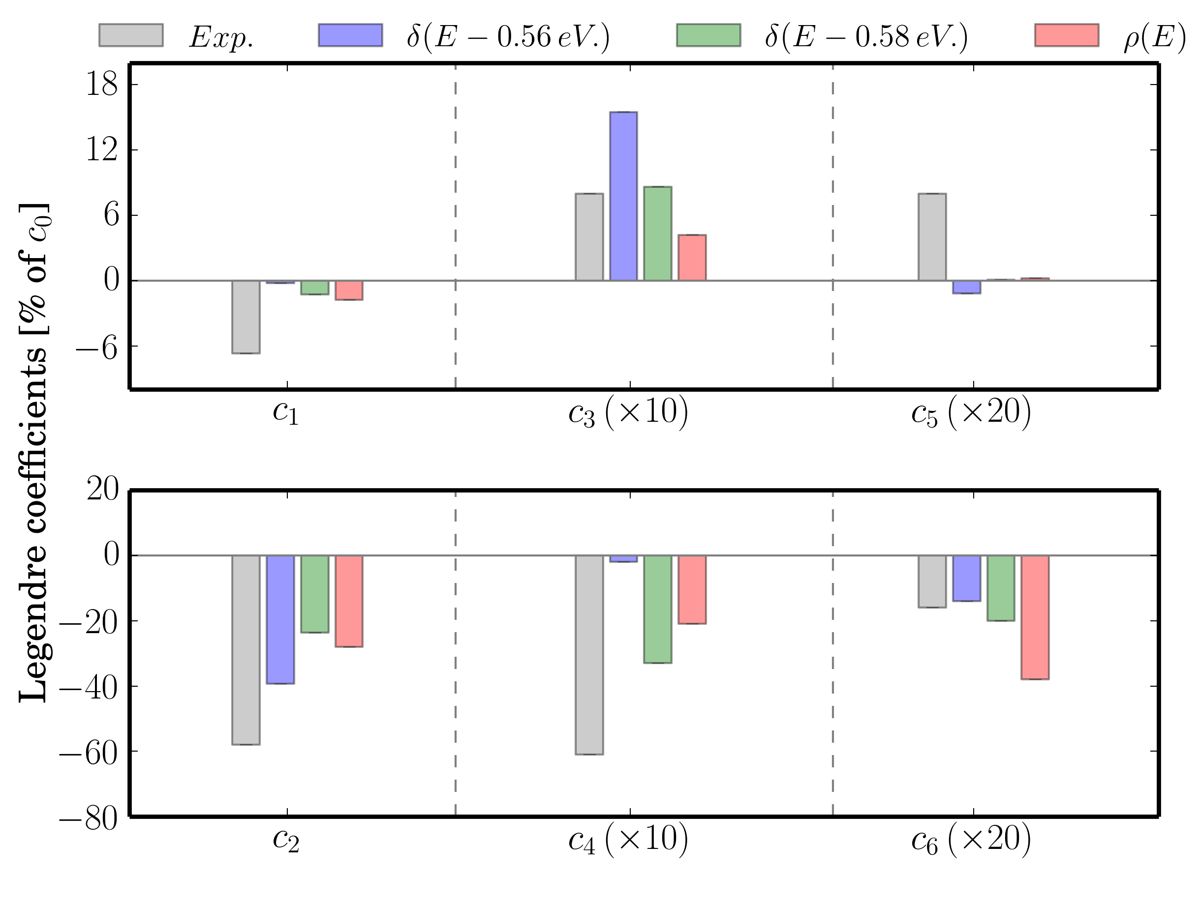
The semi-quantitative agreement between theory and experiment is further illustrated in Fig. 4 where we compare calculation results for two specific photoelectron energies, eV and eV, to the experimentally obtained Legendre coefficients. The differences for the Legendre coefficients for eV and eV indicates the dependence of our results on the error bar of the calculated excitation energy of the intermediate electronically excited state. Additionally, Fig. 4 also shows the result of integrating over a normal distribution of photoelectron energies centered at eV with a full width at half maximum (FWHM) of 200 meV. This accounts for the experimental averaging over photoelectron energies [4]. The disagreement between theoretical and experimental results amounts to a factor of about two which translates into a “mean” PECD of 3% and 4% for the fixed and adjustable tensor elements, respectively, compared to the experimental value of 10.1% [4].
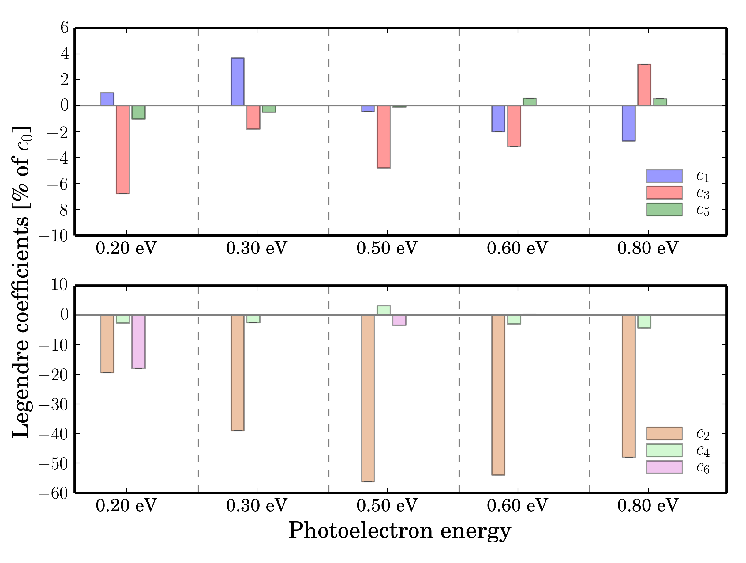
The dependence of the calculated Legendre coefficients on the photoelectron energy is investigated in more detail in Fig. 5. A non-monotonic behavior is observed for all orders. Such a non-monotonic behavior of the Legendre coefficients as a function of the photoelectron energy has already been reported for in the one-photon ionization of randomly oriented molecules [53]. It reflects the dependence of the Legendre coefficients on the radial part of the photoelectron wavefunction.
| hydrogenic continuum functions | plane waves | ||||||||||||||
|---|---|---|---|---|---|---|---|---|---|---|---|---|---|---|---|
| photoelectron energy (eV) | photoelectron energy (eV) | ||||||||||||||
| coeffs. | exp. [4] | ||||||||||||||
This dependence is studied further in Table 13, where we compare the Legendre coefficients obtained with the Kummer confluent functions, i.e., the hydrogenic continuum wavefunctions defined Appendix A.1, to those obtained with plane waves. The latter completely neglect the Coulomb interaction between photoelectron and photoion. The plane waves clearly fail to reproduce the experimentally observed PECD, see in particular the values for eV. Moreover, their values vary drastically with photoelectron energy. This difference is most likely explained by the highly oscillatory nature of plane waves even at short distances, in contrast to the hydrogenic scattering functions. Our finding is in line with the observation of Ref. [17] for the strong field approximation where plane waves fail completely to produce any PECD. In our model, non-zero odd Legendre coefficients are obtained, but a description of the photoelectron continuum that accounts for the Coulomb interaction between photoelectron and photoion provides clearly better results.
IV.2 Camphor
| state B | state C1 | state C2 | state C3 | |||||||||||||||
|---|---|---|---|---|---|---|---|---|---|---|---|---|---|---|---|---|---|---|
| coeffs. | exp. [4] | waves | waves | waves | waves | waves | waves | waves | waves | |||||||||
We now turn to camphor, for which the experimentally recorded photoelectron spectrum peaks at eV [4]. Analogously to our discussion for fenchone, we first investigate possible candidates for the intermediate resonance by considering the respective two-photon tensor alone and treating the excited state expansion coefficients as free optimization parameters. The results are displayed in Table 14, comparing the optimization that targets only the odd Legendre coefficients to that considering both odd and even . For all states, a non-zero coefficient is only obtained by including -waves in the electronically excited state (corresponding to ), as expected. When expanding up to -waves, all four candidates allow for odd Legendre coefficients close to the experimental ones, unlike the case of fenchone, where state B could already be ruled out at this stage. However, states C2 and C3 do not allow for the correct sign of , when the optimization targets both odd and even Legendre coefficients.
| state B | state C1 | state C2 | state C3 | |||||||||||||||
|---|---|---|---|---|---|---|---|---|---|---|---|---|---|---|---|---|---|---|
| coeffs. | exp. [4] | fixed | error bars | fixed | error bars | fixed | error bars | fixed | error bars | |||||||||
| state B | state C1 | state C2 | state C3 | |||||||||||||||
|---|---|---|---|---|---|---|---|---|---|---|---|---|---|---|---|---|---|---|
| coeffs. | exp. [4] | fixed | error bars | fixed | error bars | fixed | error bars | fixed | error bars | |||||||||
Once again, the ultimate test to rule out a given state consists in using both two-photon tensor elements and excited state expansion coefficients obtained from the ab initio calculations. The corresponding results are shown in Table 15. First of all, Table 15 confirms that states C2 and C3 are not the intermediate resonance probed in the experiment, since both states yield the wrong sign for both and . Comparing the remaining two candidates, states B and C1, a much better agreement is observed for C1 which yields the correct signs for all Legendre coefficients. In contrast, state B only yields correct signs for the lower orders, , , and . When accounting for the error bars in the two-photon tensor, a correct sign is additionally obtained for , but the signs for and still cannot properly be reproduced with state B as intermediate resonance. As to the state C1, not only all signs but also the correct order of magnitude for , and is observed, whereas the values are too small by one order of magnitude for and by two orders for and too large by one order of magnitude for . Allowing the two-photon absorption tensor for state C1 to vary within an error range of does not yield any significant improvement. It therefore does not seem to be the unavoidable error in the two-photon tensor elements that is important.
A second source of error in the ab initio calculations is found in the excitation energy of the intermediate electronically excited state. This is reflected in the photoelectron energy. We thus present results for a second photoelectron energy, 0.58 eV in Table 16. For state C1, all signs still match, and the correct order of magnitude is now obtained for to . In particular, is now in quantitative agreement with the experimental value, and and differ by less than factor of 1.5, respectively 2.5. Despite the disagreement in the numerical values for and , C1 is clearly the state the best matches the experimental data—the results obtained for states B, C2 and C3 show the same deficiencies as in Table 15.
| coeffs. | exp. [4] | fixed | ||||||||
|---|---|---|---|---|---|---|---|---|---|---|
The agreement with the experimental data obtained for state C1 can be further improved by allowing for larger error bars in the two-photon tensor elements. This is demonstrated in Table 17. In fact, the agreement can be made fully quantitative, except for , when increasing the error bars up to 50%, as indicated by the small value of the optimization functional. In comparison to fenchone, cf. Table 12, minimization results in significantly smaller values for , as the error range is increased. Also, the higher order Legendre coefficients are found to be more sensitive to modifications of the two-photon tensor elements than the lower ones. This is not surprising since the higher order coefficients depend more strongly on the anisotropy induced by the two-photon absorption. Analogously to fenchone, has the correct sign but remains too small by one order of magnitude. This indicates once more that we underestimate significantly the -wave contribution to the intermediate electronically excited state. It amounts to just 6% for both fenchone and camphor in our calculations.


The discussion above is summarized and illustrated in Fig. 6 which shows, besides the Legendre coefficients for photoelectron energies of 0.52 eV and 0.58 eV, those obtained when integrating over a normal distribution of photoelectron energies, centered at 0.52 eV, with a FWHM of 200 meV. The latter mimicks the spectral bandwidth in the experiment. Introducing a distribution of photoelectron energies slightly worsens the agreement between theory and experiment. This can be attributed to the striking sensitivity of the Legendre coefficients on photoelectron energy, as shown in Fig. 7. A further improvement of the theoretical model would thus require experimental data for more than one photoelectron energy and with better energy resolution.
IV.3 Discussion and Summary
Before concluding our paper, we briefly summarize our main findings. Our model describing the one-photon photoionization of an ”initial” state that is prepared by non-resonant, orientation-dependent two-photon absorption using a single-center approximation of the photoelectron continuum and ideas from optimal control allows for PECD as defined in Eq. (44) of up to 35%. This is, within our model, the maximum PECD that could be expected for an ensemble of randomly oriented chiral molecules. The upper limit is below 100% is due to the random orientation of the molecules and, possibly, due to the underlying approximations made within our model. One might thus speculate whether a better treatment of e.g. static exchange or contributions from the magnetic dipole interaction would allow for raising this limit even higher. It is, at any rate, already significantly higher than the largest PECD observed experimentally so far [1, 2, 3, 4, 5]. This encourages studies of molecules beyond bicyclic ketones, both experimentally and theoretically.
Our model accounts for the electronic structure of the experimentally investigated examples of fenchone and camphor in terms of their two-photon absorption tensor and intermediate electronically excited state based on ab initio calculations. In both cases, there are several candidate electronic states which could serve as the intermediate resonance. For fenchone, knowledge of the two-photon tensors of the candidate states alone already suggests state C3 to be the intermediate resonance. Calculations employing both two-photon tensors and excited state wavefunctions confirm this conjecture, in particular if the calculations account for error bars in the two-photon tensor. Compared to the other electronically excited states that could be accessed by the two-photon excitation, state C3 has a much larger -wave component than all other states. The largest disagreement is observed in the Legendre coefficient , suggesting that our model underestimates the -wave component of state C3. For the lower order Legendre coefficients, a semi-quantitative agreement between theoretical and experimental values is obtained.
We find proper account of the Coulomb interaction between photoelectron and photoion to be crucial. When replacing, in our expansion of the photoelectron continuum wavefunction, hydrogenic basis functions by plane waves, no agreement with the experimental values is obtained. This is in line with an earlier study of PECD using the strong-field approximation [17], where plane waves completely fail to produce any PECD.
In contrast to fenchone, knowledge of the two-photon tensors for camphor is not sufficient to point to a single state as the intermediate resonance. However, calculations accounting for the ab initio two-photon absorption matrix elements and excited state wavefunctions strongly suggest state C1 to be the intermediate resonance, in particlar when including error bars of the two-photon absorption tensor. The agreement is found to depend very strongly on the photoelectron energy, with semi-quantitative agreement found for a slightly larger value than the experimental one. Such an energy shift could be explained by the error bars of the calculated excitation energy or by the dynamic Stark shift, which is neglected in our model.
V Conclusions & Outlook
We have derived a theoretical model to study PECD after (2+1) resonantly enhanced multi-photon ionization in randomly oriented chiral molecules. The model is based on a perturbative treatment of the light-matter interaction within the electric dipole approximation and combines an ab initio description of the non-resonant two-photon absorption with a single-center expansion of the photoelectron wavefunction into hydrogenic continuum functions. This allows to account for the Coulomb interaction between photoelectron and photoion as well as electronic correlations in the transition to the intermediate electronically excited state. It neglects static exchange and dynamic correlations in the interaction of the photoelectron with the parent ion as well as the time-dependence of the laser pulse and the possible multi-center character of the continuum wavefunction. The model correctly reproduces the basic symmetry behavior expected under exchange of handedness and exchange of light helicity.
Making use of the fundamental selection rules for two-photon absorption and one-photon ionization, we have shown which Legendre coefficients may be expected in the photoelectron angular distributions, depending on the basic geometric properties in the electronic structure of the molecules as well as the possible combinations of polarization for two-photon absorption and one-photon ionization. We have identified the role of the two-photon absorption tensor and intermediate state wavefunction—it is the partial wave decomposition of the latter which determines PECD whereas the two-photon absorption tensor (in the electronic dipole approximation) merely introduces an anisotropic distribution of photoexcited molecules. Notably, the anisotropy is achieved by selection and not by rotational dynamics which would occur on a much slower timescale than that of femtosecond laser excitation.
We have applied our theoretical framework to fenchone and camphor, which have been studied extensively in recent experiments [1, 2, 3, 4, 5]. The ab initio calculations employed the coupled cluster method as well as density functional theory. Due to the Rydberg-like character of the intermediate electronically excited state, diffuse basis functions needed to be added to the standard basis sets. This has allowed to reach a reasonable agreement with experimental values for the excited state energies.
We have used the electronic structure data to calculate the photoionization cross section. Accounting for the basic structure of the two-photon absorption tensor alone has already allowed us to qualitatively reproduce the experimental results for fenchone and camphor. The minimal requirement was identified to be a contribution of -waves in the intermediate electronically excited state. Such a contribution can be expected if the two-photon absorption tensor is anisotropic. Employing the ab initio data in the calculation of the photoelectron angular distribution, we have obtained a semi-quantitative agreement between theoretical and experimental Legendre coefficients characterizing the photoelectron angular distribution.
The satisfactory agreement of our model with the experimental data encourages a number of follow-up studies. First of all, a fully time-dependent description should be employed, following the lines of Ref. [54], because the photoelectron angular distributions depend on the polarization as well as the dynamics [53]. Based on the model developed here, an extension to time-dependent studies is straightforward, but will require substantial numerical effort. Such an extension will allow to investigate the dependence of the photoelectron angular distribution on the laser parameters, including intensity, central frequency, spectral bandwidth and varying polarization. The latter would be a first step towards the coherent control of PECD.
In parallel to accounting for time-dependent effects, the electronic structure treatment may be improved. In particular, the multi-center character of the continuum wavefunction can be accounted for by employing Dyson orbitals in the calculation of the photoionization cross section [55, 31, 56]. Moreover, a perturbative treatment of the static exchange for the photoelectron and extension to beyond the electric dipole approximation should be straightforward. The former would allow for a detailed study of the dependence of the angular distribution on the photoelectron energy, including low photoelectron kinetic energies. It would thus open the way toward investigating the role of the chiral ionic core in the dynamics leading to the photoelectron angular distributions. An extension to beyond the electric dipole approximation would allow for a unified theoretical treatment of further observables beyond PECD, such as circular dichroism in laser mass spectrometry of photoions [57, 58, 59], as well as comparison with different levels of electronic structure theory [60].
Acknowledgements.
We would like to thank Christian Lux and Thomas Baumert for discussions as well as Sebastian Marquardt and Hauke Westemeier for help and discussions. Financial support by the State Hessen Initiative for the Development of Scientific and Economic Excellence (LOEWE) within the focus project Electron Dynamic of Chiral Systems (ELCH) is gratefully acknowledged.Appendix A Wavefunctions and rotation matrices
In the following, we summarize for completeness the properties of the continuum wavefunctions, rotation matrices and complex spherical harmonics in Secs. A.1, A.3 and A.4 that were used in the calculations in the main body of the paper.
A.1 Radial continuum wavefunctions of the hydrogen atom
An explicit expression of the radial continuum wavefunctions is given in terms of the Kummer confluent hypergeometric functions [25],
| (46) |
The factor
where refers to the Euler Gamma function, ensures proper normalization such that
In order to avoid numerical instabilities when generating the radial continuum wavefunctions, Eq. (46) may be written in integral form [61],
| (47) | |||||
A.2 Bound state wavefunctions of the hydrogen atom
As for the radial part of bound states for hydrogenic wavefunctions, , cf. Eq. (2), they can also be expressed in terms of the Kummer confluent hypergeometric functions [61],
| (48a) | |||||
| with | |||||
| (48b) | |||||
| where , and refer to the masses of the electron and that of the nucleous and the Bohr’s radius, respectively. | |||||
A.3 Rotation matrices
We summarize here some useful properties that are utilized in the derivation of the photoionization cross section, following the standard angular momentum algebra as found in Refs. [32, 33, 25, 34, 35]. Any irreducible tensor field of rank is transformed from the molecular frame to the laboratory frame as follows [32, 33]:
| (49) | |||||
where refers to the Wigner rotation matrix of rank , and the subscripts and stand for the projection of the total angular momentum onto the axis in the molecular, respectively laboratory, frame. Conversely, the inverse of the transformation (49) is given by
| (50) | |||||
We express all vector quantities in spherical coordinates,
| (51) |
where refers to the spherical unit vector in the laboratory frame, and denotes linear, left and right unit components, respectively. The correspondence between the components of a arbitrary vector operator in spherical and cartesian basis is given by [32, 33, 62],
Transforming the spherical components , with in to the Cartesian basis using Eq. (A.3) and Eq. (104), we find the two-photon absoption tensor in the spherical basis,
Because , with , cf. Eq. (104), it can be straightforwardly shown, using Eq. (A.3), that .
In the derivations we make heavily use of the product rule for two Wigner rotations matrices of ranks and ,
| together with the following symmetry property, | |||||
| (63b) | |||||
where denotes the complex conjugate.
A.4 Conversion to complex spherical harmonics
The standard complex spherical harmonics are related to the real spherical harmonics by
| Therefore the excited state expansion coefficients , defined in Eq. (2), are connected to the coefficients in the basis of real spherical harmonics by | |||
The naming of the real spherical harmonics used in the reexpansion of the molecular wavefunctions is explained in Table 18.
| designation | real spherical harmonic | |
|---|---|---|
Appendix B Derivations
Here, we provide details of the derivation of the one-photon transition rate, two-photon absorption tensor and the photoionization cross section in Secs. B.1 to B.3 as well as the behavior of the Legendre coefficients under change of helicity in the one-photon photoionization and two-photon absorption processes in Secs. B.4 to B.6.
B.1 One-photon transition rate
This section is devoted to deriving the rate for the photoionization transition from the intermediate electronically excited state to the continuum, driven by an electric field with polarization . The starting point is the doubly differential cross section in the molecular frame given in Eq. (7). It contains the laboratory-frame product , which, using Eq. (51), becomes
| (65) |
This is rotated into the molecular frame, employing Eq. (49), resulting in
| (66) |
Inserting Eq. (66) into Eq. (7) yields the photoionization cross section in the molecular frame as a function of the Euler angles , cf. Eq. (8). Evaluating Eq. (8) requires evaluation of the product . Inserting Eqs. (4) and (7) yields, for a fixed polarization direction ,
with and defined in Eqs. (10a) and (10b) such that Eq. (8) comprises the product . Using the symmetry properties of the spherical harmonics, we can write
| (67a) | |||||
| with | |||||
| (67b) | |||||
and refering to polar and azimuthal angles of the momentum vector in the molecular frame of reference. In order to express the photoionization direction in the laboratory frame, we need to apply the inverse transformation (50) to , i.e.,
| (68a) | |||||
| Using Eq. (68a), Eq. (67a) then becomes, | |||||
| (68b) | |||||
with
| (69) |
In Eq.(68), we have used the equality between spherical harmonics and associate Legendre polynomials, including the Condon-Shortley phase convention [32, 25, 62],
Inserting Eq. (68) into Eq. (9), we obtain the differential one-photon cross section in the laboratory frame of reference for a fixed molecular orientation defined in Eq. (11).
B.2 Two-photon absorption tensor
The probability of two-photon absorption, Eq. (), of a molecule that is oriented with angles with respect to the laboratory frame of reference contains the product . Using Eqs. (63), we obtain
| (71a) | |||
| and analogously for , | |||
| (71b) | |||
Inserting Eqs. (71) into () and using
with , the orientation-dependent probability of two-photon absorption becomes,
| (72) | |||||
cf. Eq. (19). Two useful properties of the Wigner symbols utilized throughout this work, involve odd permutations of two columns [35],
| (73) |
as well as the unitary condition for the Wigner rotation matrices [35],
| (74) |
B.3 Cross section for photoionization
In order to simplify the expression of the cross section for the (2+1) REMPI process, we utilize the properties defined in Eq. (63), to the product involving the first and second Wigner symbols in Eq. (11),
| (75) |
This allows for exploiting, in the integration over the Euler angles, the well-known properties for integrating over a product of three Wigner symbols. With Eq. (75), Eq. (11) takes the following form,
| (76) | |||||
Inserting Eq. (72) and Eq. (76) into Eq. (12), the PAD measured in the laboratory frame, resulting from a fixed molecular orientation reads,
| (77) | |||||
with . Equation (77) may be written in the more compact form of Eqs. (20), namely,
| (78a) | |||||
| In Eq. (78a), the only orientation-dependent quantity, , is given by | |||||
| (78b) | |||||
with defined as
| (79) | |||||
where comprises all summation indices, except for and , as described in Sec. B.3. Next, according to Eq. (13), we need to average over all initial orientations, i.e., integrate the doubly differential cross section over the Euler angles. To this end, we utilize the following integration property involving the product of three Wigner symbols [32, 33, 35],
| (80) |
with . Finally, following Eq. (13), integration of Eq. (77) over the Euler angles , using Eq. (80), gives the expression of the laboratory frame PAD resulting from a randomly ensemble of molecules in the context of a REMPI process, defined in Eq. (22). In particular, due to the second Wigner symbol in Eq. (80), it is clear that the integral vanishes if . As a consequence, this requirement translates into cylindrical symmetry of the PAD measured in the laboratory frame, as also appears in the azimuthal angle dependent term in Eq. (77). Thus, we retrieve the expression defined in Eq. (22).
B.4 Non-zero Legendre coefficients for two-photon absorption with circularly polarized light and ionization with linear polarization
In this section, we show that a REMPI process for which the two-photon absorption process is driven by circular polarized light, followed by linearly polarized light for the radiative process, lead within the electric dipole approximation exclusively to even Legendre coefficients. To this end, we exploit the symmetry as well as invariance properties of Eq. (22b), by making a change of variables for , , and in Eq. (22b) that preserves unchanged and also keeps invariant (in order to keep the fifth Wigner symbol in Eq. (22b) unchanged). A change of variables fulfilling this property reads,
| (81) |
i.e. it interchanges and .
For simplicity, we define the quantity,
| (82a) | |||||
| with | |||||
| (82b) | |||||
Eqs. (82) appear in Eq. (22b). In Eq. (82), and stands for the indices . Analogously, is defined using the primed dummy variables , for with the symmetry property . Of course, we have,
| (83) |
Using Eq. (81), the tensor elements appearing in Eq. (22b) then transform according to
| (84a) | |||
| and | |||
Using Eq. (84), Eq. (82) reads, upon transformation,
| (85) | |||||
with . Next, we evaluate the quantity present in Eq. (85) using Eq. (19b), we find
| (86) | |||||
where we have interchanged the dummy indices and . Application of Eq. (26) to the first and third Wigner symbol in Eq. (86) gives,
| (87a) | |||||
| and | |||||
| (87b) | |||||
| respectively. Next, we permute the first and second column in the fifth Wigner symbol in Eq. (86), following Eq. (73), which yields | |||||
| (87c) | |||||
Finally, inserting Eqs. (87) into Eq. (86) together with the property , we find
with invariant as invariant, and where is defined in Eq. (19b). Eq. (B.4) means that the summations over and is invariant under the transformation . Using Eq. (B.4), we find for and ,
| (89) | |||||
In Eq. (89), the factors and arise from Eqs. (B.4) and from application of the property defined in Eq. (26) to the sixth Wigner symbol in Eq. (89), respectively. Furthermore, we used the property that is even, i.e. only even contribute to the summation, due to the triple zeros in the second row of the fourth Wigner symbol. Finally, using Eq. (83), it follows that for ,
| (90) |
Because no assumptions have been made on the polarization direction , Eq. (90) shows that only even Legendre coefficients are present in the PAD if the radiative photoabsorption is driven by linearly polarized light, i.e. , independently of the polarization direction, , driving the non-resonant two-photon absorption process. As a consequence, only even Legendre orders contribute to the PAD if and , translating into a vanishing PECD.
B.5 Behavior of Legendre coefficients when changing the helicity of the one-photon photoionization
The easiest way to prove Eq. (36) consists of making the change of variables defined in Eq. (81), and evaluate , using the property
| (91) |
where the unprimed (primed) quantities in Eq. (91) refer to the Legendre coefficients before (after) the change of variables, respectively.
Keeping is fixed while changing the polarization direction transforms the fourth Wigner symbol in Eq. (22b) according to,
| (92) |
| (93) | |||||
In Eq. (93), the factors and arise from the invariance property defined in Eq. (B.4) for the transformation defined in Eq. (81), and (92), respectively. Application of the property defined in Eq. (26) to the sixth Wigner symbol in Eq. (93) gives rise to the factor . The terms in and compensates, giving rise to the factor in alone. Finally, using (91) and comparing Eq. (22b) for and and Eq. (93) for and , determines the proof for Eq. (36), i.e.,
| (94) |
B.6 Behavior of Legendre coefficients when changing the helicity of the two-photon absorption process
In this section, we present the proof of Eq. (37). To verify that it is the polarization direction of the ionizing field alone which imposes the sign for all odd Legendre coefficients, whereas the polarization direction of the two-photon absorption plays no role, we define the following transformation
| (95) |
which interchanges the indices and while keeping Eq. (22b) unchanged and invariant. In particular, the tensor elements appearing in Eq. (22b) then transform according to,
| (96a) | |||||
| and | |||||
| (96b) | |||||
where we have made use of the correspondence between the components of a vector operator in spherical and cartesian basis, defined in Eq. (A.3) in Appendix A.3, in , for , together with the fact that the two-photon absorption tensor is symmetric in cartesian coordinates, i.e., for .
We define , according Eq. (82) and we study the symmetry properties of upon transformation defined in Eq. (95). In particular, because the quantity given by,
| (97) |
is (as for the earlier transformation defined in Eq. (81)) invariant under transformation defined in Eq. (95), we may neglect it in the following, avoiding cumbersome notations. We outline, however, that a full notation was used in Section B.4. Therefore, given such invariance properties, we may consider the behavior of under exchange alone, and neglect the extra terms depending on in the expression for . Because is changed to while is kept fixed, we consider which becomes, upon transformation defined in Eq. (95),
| (98) | |||||
where we have interchanged the indexes and . Next we apply the symmetry property given in Eq. (26), followed by an odd permutation of the first and second columns, according to Eq. (73), to the first Wigner symbol in Eq. (98). We find,
| (99a) | |||||
| The same procedure is applied to the third symbol in Eq. (98), i.e., | |||||
| (99b) | |||||
| Next, odd permutation of the first and second columns in the fifth Wigner symbol gives, | |||||
| (99c) | |||||
| Application of Eq. (26), followed by permutation of the first two rows leaves the sign of the second Wigner symbol unchanged for all , namely | |||||
| (99d) | |||||
| and analogously for the fourth Wigner symbol involving . It is to note that, the left side of Eq. (99d) is related to while the right side is related to . | |||||
Appendix C Evaluation of the two-photon transition moments in the framework of coupled cluster theory
The rotationally averaged two-photon transition strength strength (in a.u.) and the two-photon transition probability rate constant are defined in units of as follows [63, 64, 65, 66]
| (101a) | |||||
| (101b) | |||||
where is the Bohr radius, is the atomic unit of time, the fine structure constant and and the photon energies. , and are parameters depending on the arrangement and polarization of the laser used in the experiment [63, 64, 65, 66]. In Eq. (101a), the parameters , and read [63, 65]
| (102) |
where and . Here and refer to the ground and excited states. In the above relations, , the so-called transition strength, is defined as follows [63, 65]
| (103) | |||||
where the and are called the two-photon transition matrix elements. These tensors read [63, 65]
| (104) |
where and are Cartesian components of the position operator ( and ). and are the photon energies which satisfy the matching condition . For variational ab initio methods, the two-photon absorption tensor is symmetric with respect not only to the permutation of the operators and (assuming that is replaced by ) but also to complex conjugation combined with a simultaneous inversion of the frequencies and exchange of the initial and final states [63, 65]. In coupled cluster response theory, the two-photon absorption tensors and are are in general not each other complex conjugate i.e. , whereas for the transition strengths, which are calculated as a symmetrized product of right and left two-photon absorption tensors as shown in Eq. (103), we have [63, 65]
| (105) |
These two-photon absorption tensors and are called right and left two-photon absorption tensor from the ground state to the excited state , respectively [63, 65]. As a side remark, the imaginary part of two-photon absorption tensors calculated using the CC method vanishes in the limit of complete cluster expansion and thus it does not influence the results of the two-photon absorption tensor [67].
We should mention that Eq. (104) is presented in a general form and in the Cartesian basis. However, we interest in the special case two photons with same polarization and energy values (i.e. ). If one uses the inverse relations of Eq. (A.3) and inserts them into Eq. (104), it will give Eq. (), which is two-absorption tensor in the spherical basis.
The left and right two-photon absorption tensors change under a rotation , whereas the transition strength remain unchanged (). The left and right two-photon absorption tensors for fenchone and camphor (calculated at the rotated arrangement (see Fig. 1) such that the origin is at the center of mass and principal axes of inertia are along coordinate axes) are shown in Tables 20 and 21. In Fig. 1, the eigenvectors of the left (red vectors) and right (blue vectors) two-photon absorption tensor corresponding to the third electronically excited states of fenchone and camphor are shown. The corresponding eigenvalues of the left and right two-photon absorption tensor are and , respectively for fenchone and and , respectively for camphor. From this information, the rhombicity (), axialty () and the ratio () of these symmetric tensors can be calculated using the following relations:
| (106) |
where b and e are
| (107) |
Here refers to the left and right two-photon absorption tensors and and refers to the diagonal elements of the the left and right two-photon absorption tensors. Based on Eq. (106), the corresponding numerical values for the rhombicity (), axiality () and an their ratio () are shown in Table. 19.
| fenchone | camphor | |||
|---|---|---|---|---|
| left | right | left | right | |
As inferred from Table. 19, these values for fenchone and camphor are close to each other. Furthermore, we report the parameters , , , and for different types of polarisations in Tables 22, 23, 24 and 20.
| States | ||||||||||||
|---|---|---|---|---|---|---|---|---|---|---|---|---|
| A | ||||||||||||
| B | ||||||||||||
| States | ||||||||||||
|---|---|---|---|---|---|---|---|---|---|---|---|---|
| A | ||||||||||||
| B | ||||||||||||
| states | 11 1 both photon circularly polarized i.e., F=- 1 4 ,G= 7 2 and H=- 1 4 | 22 2 both photon circularly polarized i.e., F=- 1 4 ,G= 7 2 and H=- 1 4 | |||
|---|---|---|---|---|---|
| A | |||||
| B | |||||
| states | 33 3 both photons polarized linearly with parallel polarization i.e., F=G=H=2 | 44 4 both photons polarized linearly with parallel polarization i.e., F=G=H=2 | 55 5 both photons polarized linearly with perpendicular polarization i.e., F=-1,G=4 and H=-1 | 66 6 both photons polarized linearly with perpendicular polarization i.e., F=-1,G=4 and H=-1 |
|---|---|---|---|---|
| A | ||||
| B | ||||
| states | 77 7 both photon circularly polarized i.e., F=- 1 4 ,G= 7 2 and H=- 1 4 | 88 8 both photon circularly polarized i.e., F=- 1 4 ,G= 7 2 and H=- 1 4 | |||
|---|---|---|---|---|---|
| A | |||||
| B | |||||
| states | 99 9 both photons polarized linearly with parallel polarization i.e., F=G=H=2 | 1010 10 both photons polarized linearly with parallel polarization i.e., F=G=H=2 | 1111 11 both photons polarized linearly with perpendicular polarization i.e., F=-1,G=4 and H=-1 | 1212 12 both photons polarized linearly with perpendicular polarization i.e., F=-1,G=4 and H=-1 |
|---|---|---|---|---|
| A | ||||
| B | ||||
As indicated, there are two two-photon transition matrices obtained when we employ the coupled cluster method. This is problematic in the calculation of photoelectron angular distributions of the molecules under investigations, because the model constructed for this purpose (see Sec. II) depends on only a single two-photon transition tensor. Thus, the computational procedure based on the CC calculation would not work for the evaluation of photoelectron angular distributions, unless the left and right two-photon transition tensors are combined such that the two-photon transition strength and the total cross section remain unchanged when compared to the conventionally chosen recipe for coupled cluster calculations.
The effective two-photon transition matrix element can be written as follows,
| (108) |
and the of being the same as the signs of the left and right two-photon absorption tensors for each electronic state as shown in Tables 20 and 21.
Employing Eq. (108) leaves the transition strength of and the two-photon transition probability rate constant unchanged. Thus all parameters , , , as well as in Eqs. (101) and (102) are the same as before combining the right and left transition moments. Thus, employing Eq. (108) provides exactly the same reported values in Tables 22, 23, 24 and 20. The lower part of Tables 8 and 9 presents the (symmetric) effective two-photon transition matrix elements (transition moments) based on Eq. (108) for fenchone and camphor.
References
- [1] C. Lux, M. Wollenhaupt, T. Bolze, Q. Liang, J. Köhler, C. Sarpe, and T. Baumert, Angew. Chem. Int. Ed. 51, 4755 (2012).
- [2] C. S. Lehmann, N. B. Ram, I. Powis, and M. H. M. Janssen, J. Chem. Phys. 139, 234307 (2013).
- [3] M. H. M. Janssen and I. Powis, Phys. Chem. Chem. Phys. 16, 856 (2014).
- [4] C. Lux, M. Wollenhaupt, C. Sarpe, and T. Baumert, ChemPhysChem 16, 115 (2015).
- [5] M. M. Rafiee Fanood, M. H. M. Janssen, and I. Powis, Phys. Chem. Chem. Phys. 17, 8614 (2015).
- [6] B. Ritchie, Phys. Rev. A 13, 1411 (1976a).
- [7] I. Powis, “Photoelectron circular dichroism in chiral molecules,” in Advances in Chemical Physics (John Wiley & Sons, Inc., 2008) pp. 267–329.
- [8] L. Nahon and I. Powis, in Chiral Recognition in the Gas Phase, edited by A. Zehnacker (CRC Press, 2010).
- [9] S. N. Dixit and P. Lambropoulos, Phys. Rev. A 27, 861 (1983).
- [10] P. R. Monson and W. M. McClain, J. Chem. Phys. 53, 29 (1970a).
- [11] P. R. Monson and W. M. McClain, J. Chem. Phys. 53, 29 (1970b).
- [12] W. M. McClain, J. Chem. Phys. 57, 2264 (1972).
- [13] W. M. McClain, Acc. Chem. Res 7, 129 (1974).
- [14] I. Tinoco Jr., J. Chem. Phys. 62, 1006 (1974).
- [15] L. V. Keldysh, Sov. Phys. JEPT 20, 1307 (1965).
- [16] F. H. M. Faisal, J. Phys. B 6, L89 (1973).
- [17] I. Dreissigacker and M. Lein, Phys. Rev. A 89, 053406 (2014).
- [18] Z. Amitay, A. Gandman, L. Chuntonov, and L. Rybak, Phys. Rev. Lett. 100, 193002 (2008).
- [19] L. Rybak, S. Amaran, L. Levin, M. Tomza, R. Moszynski, R. Kosloff, C. P. Koch, and Z. Amitay, Phys. Rev. Lett. 107, 273001 (2011).
- [20] L. Levin, W. Skomorowski, L. Rybak, R. Kosloff, C. P. Koch, and Z. Amitay, Phys. Rev. Lett. 114, 233003 (2015).
- [21] B. Ritchie, Phys. Rev. A 13, 1411 (1976b).
- [22] K. L. Reid., Annu. Rev. Phys. Chem 54, 397 (2003).
- [23] J. Cooper and R. N. Zare, in Lectures In Theoretical Physics, Vol. 9, edited by Gordon and Breach (University of Colorado, New York, 1968) pp. 317–337.
- [24] N. Chandra, J. Phys. B 20, 3405 (1987).
- [25] H. A. Bethe and E. E. Salpeter, Quantum Mechanics of One and Two-Electron Atoms, 1st ed. (Academic Press Inc., 111, Fifth Avenue, New York 3, New York/USA, 1957).
- [26] C. Jin, A.-T. Le, S.-F. Zhao, R. R. Lucchese, and C. D. Lin, Phys. Rev. A 81, 033421 (2010a).
- [27] R. R. Lucchese, G. Raseev, and V. McKoy, Phys. Rev. A 25, 2572 (1982).
- [28] B. M. Bishop, Advances in Quantum Chemistry, 1st ed., Vol. 3 (Academic Press Inc., Berkeley Square House, London W.1, 1967).
- [29] C. Jin, A.-T. Le, S.-F. Zhao, R. R. Lucchese, and C. D. Lin, Phys. Rev. A 81, 033421 (2010b).
- [30] D. Dill, J. Chem. Phys. 65, 1130 (1976).
- [31] C. M. Oana and A. I. Krylov, J. Chem. Phys. 131, 124114 (2009).
- [32] A. Edmonds, Angular Momentum in Quantum Mechanics, 4th ed. (Princeton University Press, Princeton, New Jersey, 1996).
- [33] B. L. Silver, Irreducible Tensor Methods: An Introduction or Chemists, 1st ed., Vol. 36 (Academic Press, Inc.(London) LTD, 24/28 Oval Road, London NW1, 1976) an optional note.
- [34] M. Rose, Elementary Theory of Angular Momentum, 5th ed. (John Wiley & Sons, Inc., New York, 1967).
- [35] D. Varshalovich, A. Moskalev, and V. Khersonskii, Quantum Theory of Angular Momentum: Irreducible Tensors, Spherical Harmonics, Vector Coupling Coefficients, 3nj Symbols, 1st ed. (Word Scientific Co. Pte. Ltd., 687 Hartwell Street, Teaneck, NJ 07666, 1988).
- [36] W. L. Peticolas, Annu. Rev. Phys. Chem. 18, 233 (1967).
- [37] W. M. McCLAIN and R. A. HARRIS, in Excited States, edited by E. C. LIM (Academic Press, 1977) pp. 1–56.
- [38] M. A. C. Nascimento, Chem. Phys. 74, 51 (1983).
- [39] C. N. Yang, Phys. Rev. 74, 764 (1948).
- [40] J. Pollmann, R. Franke, and J. Hormes, Spectrochimica Acta Part A: Molecular and Biomolecular Spectroscopy 53, 491 (1997).
- [41] University of Karlsruhe and Forschungszentrum Karlsruhe GmbH, “TURBOMOLE 6.6 2014: program package for ab initio electronic structure calculations,” (2014).
- [42] See supplemental material at [URL will be inserted by editor] for the expansion coefficients of the intermediate state wavefunctions obtained in the single center reexpansion and the Cartesian coordinates obtained in the geometry optimization.
- [43] C. Angeli, “Dalton: a molecular electronic structure program, release 2.0,” (2015).
- [44] M. J. Paterson, O. Christiansen, F. Pawłowski, P. Jørgensen, C. Hättig, T. Helgaker, and P. Sałek, J. Chem. Phys. 124, 054322 (2006).
- [45] C. Hättig and P. Jørgensen, J. Chem. Phys. 109, 9219 (1998).
- [46] H.-J. Werner, P. J. Knowles, G. Knizia, F. R. Manby, M. Schütz, et al., “Molpro, version 2012.1, a package of ab initio programs,” (2012).
- [47] F. Pulm, J. Schramm, J. Hormes, S. Grimme, and S. D. Peyerimhoff, Chem. Phys. 224, 143 (1997).
- [48] D. E. Woon and T. H. Dunning, J. Chem. Phys. 100, 2975 (1994).
- [49] M. E. Casida, C. Jamorski, K. C. Casida, and D. R. Salahub, J. Chem. Phys. 108, 4439 (1998).
- [50] H. H. Falden, K. R. Falster-Hansen, K. L. Bak, S. Rettrup, and S. P. A. Sauer, J. Phys. Chem. A 113, 11995 (2009).
- [51] C. Diedrich and S. Grimme, J. Phys. Chem. A 107, 2524 (2003).
- [52] MATLAB, version 7.10.0 (R2014a) (The MathWorks Inc., Natick, Massachusetts, 2014).
- [53] C. J. Harding, E. Mikajlo, I. Powis, S. Barth, S. Joshi, V. Ulrich, and U. Hergenhahn, J. Chem. Phys. 123, 234310 (2005).
- [54] T. Seideman, Phys. Rev. A 64, 042504 (2001).
- [55] C. M. Oana and A. I. Krylov, J. Chem. Phys. 127, 234106 (2007).
- [56] A. Humeniuk, M. Wohlgemuth, T. Suzuki, and R. Mitrić, J. Chem. Phys. 139, 134104 (2013).
- [57] U. Boesl von Grafenstein and A. Bornschlegl, ChemPhysChem 7, 2085 (2006).
- [58] R. Li, R. Sullivan, W. Al-Basheer, R. M. Pagni, and R. N. Compton, J. Chem. Phys. 125, 144304 (2006).
- [59] H. G. Breunig, G. Urbasch, P. Horsch, J. Cordes, U. Koert, and K.-M. Weitzel, ChemPhysChem 10, 1199 (2009).
- [60] D. Kröner, Phys. Chem. Chem. Phys. 17, 19643 (2015).
- [61] C. Aslangul, Mécanique Quantique 2, Développements et applications à basse énergie, 1st ed. (De Boeck S.A, Rue des Minimes 39, B-1000, Bruxelles, 2008).
- [62] M. Abramowitz and I. A. Stegun, Handbook of Mathematical Functions with Formulas, Graphs and Mathematical Tables, 10th ed. (National Bureau of Standards, Applied Mathematics Series 55, 20402, Washington D.C./USA, 1972).
- [63] C. Hättig, O. Christiansen, and P. Jørgensen, J. Chem. Phys. 96, 8355 (1998a).
- [64] P. R. Monson and W. M. McClain, J. Chem. Phys. 53, 29 (1970c).
- [65] O. Christiansen, P. Jørgensen, and C. Hättig, Inter. J. Quan. Chem. 68, 1 (1998).
- [66] D. Sundholm, A. Rizzo, and P. Jørgensen, J. Chem. Phys. 101, 4931 (1994).
- [67] C. Hättig, O. Christiansen, and P. Jørgensen, J. Chem. Phys. 108, 8331 (1998b).