Nonparametric causal inference from observational time series through marginal integration

Shu Li ^†^†thanks: Seminar for Statistics, ETH Zürich, last name @ stat.math.ethz.ch^†^†thanks: Supported by SNF 2-77991-14 Jan Ernest¹¹footnotemark: 1 ^†^†thanks: Supported in part by the Max Planck ETH Center for Learning Systems Peter Bühlmann¹¹footnotemark: 1

Abstract

Causal inference from observational data is an ambitious but highly relevant task, with diverse applications ranging from natural to social sciences. Within the scope of nonparametric time series, causal inference defined through interventions (cf. Pearl [19]) is largely unexplored, although time order simplifies the problem substantially. We consider a marginal integration scheme for inferring causal effects from observational time series data, MINT-T (marginal integration in time series), which is an adaptation for time series of a method proposed by Ernest and Bühlmann (Electron. J. Statist, pp. 3155-3194, vol. 9, 2015) for the case of independent data. Our approach for stationary stochastic processes is fully nonparametric and, assuming no instantaneous effects consistently recovers the total causal effect of a single intervention with optimal one-dimensional nonparametric convergence rate $n^{-2/5}$ assuming regularity conditions and twice differentiability of a certain corresponding regression function. Therefore, MINT-T remains largely unaffected by the curse of dimensionality as long as smoothness conditions hold in higher dimensions and it is feasible for a large class of stationary time series, including nonlinear and multivariate processes. For the case with instantaneous effects, we provide a procedure which guards against false positive causal statements.

1 Introduction

In a time series setting, causal reasoning revolves predominantly around Granger causality [9]. Roughly speaking, a time series is Granger causal to another one if knowing the past of the former helps predict the future of the latter, given all other available information of the past (e.g., from the second or other time series). This is a concept of ”predictive causality”. Furthermore, Granger causality is measuring a direct effect, e.g., its targets are the entries of the coefficient matrix in a vector autoregressive model. Here, we are considering total causal effects describing the total effect of an intervention at a (single) variable: although less ambitious than direct effects, we will argue here that total effects are much more feasible to infer in a model-free, nonparametric way. For this task, we use the framework of causal reasoning through interventions as described by Pearl [19] or Spirtes et al. [21]. It is largely unexplored for the case of time series, although time dependence has plenty to offer in this particular setting. From our perception of time, the present is affected by the past but not vice versa. We also commonly note that causes precede their effects. Both relations are inherently asymmetric. In the simplest setting of two correlated random variables without hidden confounders, we are not able to tell apart the cause from its effect without making any additional assumptions in the i.i.d. setting. This is in contrast to time series where in general we can distinguish cause from effect by looking at the order in time thereby assuming that the time resolution of the measurements is higher than the timescale of causal influences, that is, there are no instantaneous effects [12]. In case of instantaneous effects, one can still derive some interesting statements as we discuss in Section 2.3. Time ordering is a simplification of a more general phenomenon, though. In general, the estimation of causal models in the i.i.d. case involves finding a causal ordering of random variables, and this often involves unverifiable assumptions such as faithfulness and sophisticated structure search algorithms such as GES [4], PC [21] or CAM [3]. Moreover, without making further assumptions on the data-generating process, the causal model is typically only identifiable up to an equivalence class of valid causal orderings. Within time series, we can often ignore the identifiability aspects and skip the complicated part of structure learning by simply propagating time as the causal order.

We consider the average total causal effect which is defined through Pearl’s $\mathrm{do}$ -operator [19]:

\displaystyle\mathbb{E}[X_{t}\,|\,\mathrm{do}(X_{t-s}=x)],

(1)

where the $\mathrm{do}$ -operator encodes an external intervention by setting the random variable $X_{t-s}$ to the fixed deterministic value $x$ ; here $X_{t}$ and $X_{t-s}$ are real-valued. We often refer to this quantity as the causal effect of $X_{t-s}$ on $X_{t}$ (and suppress the words ”average total”). For a stationary time series $({X}_{t})_{t\in\mathbb{Z}}$ , the causal effect is invariant under time shifts in $t$ . In case of a multivariate time series, we would consider components $X_{c_{1},t}$ and $X_{c_{2},t-s}$ in (1). The quantity in (1) is a general function of $x$ , for each value of $s$ (and in the multivariate case it also depends on $c_{1}$ and $c_{2}$ ). Our goal is to estimate this function of $x$ in a fully nonparametric way without relying on a specific model specification for the underlying time series.

A simple example should help to illustrate our goal. Consider a stationary $\mathrm{AR}(p)$ -model: $X_{t}=\sum_{j=1}^{p}\phi_{j}X_{t-j}+\epsilon_{t}$ , where $p$ is the order of the Markovian process, and we assume the $\epsilon_{t}$ ’s to be i.i.d. with mean zero and $\epsilon_{t}$ to be independent of $\{X_{s};\ s<t\}$ . Then,

\displaystyle\mathbb{E}[X_{t}\,|\,\mathrm{do}(X_{t-s}=x)]

\displaystyle=

\displaystyle\sum_{j=1}^{p}\phi_{j}\mathbb{E}[X_{t-j}\,|\,\mathrm{do}(X_{t-s}=x)].

For a fixed intervention value $x$ , the causal effect can be calculated recursively via $g_{x}(s):=\mathbb{E}[X_{t}\,|\,\mathrm{do}(X_{t-s}=x)]=\sum_{j=1}^{p}\phi_{j}g_{x}(s-j)$ with initial values $g_{x}(0)=\mathbb{E}[X_{t}\,|\,\mathrm{do}(X_{t}=x)]=x$ and $g_{x}(-s)=\mathbb{E}[X_{t}\,|\,\mathrm{do}(X_{t+s}=x)]=\mathbb{E}[X_{t}]=0$ for $s>0$ . Since $g_{x}(s)$ is a linear combination of previous $\{g_{x}(s-i)\,|\,i>0\}$ , we thus see that the causal effect $\mathbb{E}[X_{t}\,|\,\mathrm{do}(X_{t-s}=x)]$ is a linear function of the intervention value $x$ . Furthermore, $\mathbb{E}[X_{t}\,|\,\mathrm{do}(X_{t-s}=x)]$ is geometrically decaying because $g_{x}(s)$ satisfies the skeleton equation of the stationary AR(p)-model. However, if the true underlying data generating stationary process is nonlinear, perhaps with non-additive innovation terms, the causal effect is typically a nonlinear function of $x$ and such a recursive formulation is difficult and not useful for the task of estimating the causal effect.

Instead, we will use an approach based on Pearl’s backdoor adjustment formula [19]. The interventional density can be calculated from the observational density

p(x_{t}\,|\,\mathrm{do}(X_{t-s}=x))=\int p(x_{t}\,|\,X_{t-s}=x,X_{t-s}^{\mathcal{S}})dP(X_{t-s}^{\mathcal{S}}),

(2)

where $X_{t-s}^{\mathcal{S}}$ denotes a so-called adjustment set of $X_{t-s}$ , and the expression in (2) is invariant under shifts in $t$ due to the stationarity assumption. In a time series setting with a data-generating univariate Markovian process, the adjustment set can be chosen as $X_{t-s}^{\mathcal{S}}=\{X_{t-s-1},\ldots,X_{t-s-p}\}$ , the previous instances in time up to a time lag $p\in\mathbb{N}^{0}$ where the value $p$ has to be at least as large as the order of the Markovian process. Thus, for stationary Markovian processes we obtain:

\displaystyle\mathbb{E}[X_{t}\,|\,\mathrm{do}(X_{t-s}=x)]=\int\mathbb{E}[X_{t}\,|\,X_{t-s}=x,X_{t-s}^{\mathcal{S}}]dP(X_{t-s}^{\mathcal{S}}).

(3)

In particular, (3) illustrates that we can relate the causal effect to integrating the regression function $m(x,X_{t-s}^{\mathcal{S}})=\mathbb{E}[X_{t}\,|\,X_{t-s}=x,X_{t-s}^{\mathcal{S}}]$ over the adjustment variables $X_{t-s}^{\mathcal{S}}$ , and this is the key property to construct an estimator in a model free way. This line of reasoning can be extended to multivariate $l$ -dimensional time series where causal statements are often more interesting: we aim to estimate

\displaystyle\mathbb{E}[\mathbf{X}_{t}\,|\,\mathrm{do}(X_{c,t-s}=x)],

where $c\in\{1,\ldots,l\}$ denotes a single component. The same formula (3) applies when using an appropriate adjustment set $\mathbf{X}_{t-s}^{\mathcal{S}}$ . The latter will depend whether there are time-instantaneous effects across the different components or not. We show that when having no instantaneous effects, assuming regularity conditions and twice differentiability of $\mathbb{E}[\mathbf{X}_{t}\,|\,X_{c,t-s}=x,\mathbf{X}_{t-s}^{\mathcal{S}}]$ with respect to $x$ , our proposed marginal integration estimator achieves the $n^{-2/5}$ convergence rate for estimating the true causal effect $\mathbb{E}[\mathbf{X}_{t}\,|\,\mathrm{do}(X_{c,t-s}=x)]$ . In case of instantaneous effects, we will derive a conservative procedure which does not require any knowledge about the true underlying structure of the Markovian process.

1.1 Related work and our contribution

Nonparametric estimation of causal effects of continuous (intervention/treatment) random variables with marginal integration of the regression function has been proposed by Ernest and Bühlmann [6] in the i.i.d. setting. The difficulty there is that the adjustment in (2) has to be estimated from data, unless it is known. This task is rather delicate, as it amounts to determining a superset of the parents of the intervention variable in a structural equation model; and it is difficult to imagine that this could be accurately done in a nonparametric way.

Here, with Markovian time series and without instantaneous effects in multivariate settings, a valid adjustment set only needs the knowledge or a good estimate of an upper bound of the Markovian order. This makes our procedure much more reliable, and in fact, our implementation of marginal integration is somewhat different and more direct than the proposal in Ernest and Bühlmann [6]. Our investigation for the case with instantaneous effects in multivariate scenarios is novel and specific to time series problems. Regarding the mathematical analysis, the technical derivation of the convergence rate for estimating causal effects is substantially more demanding and we extend the existing theory to strongly mixing stationary multivariate processes. Thereby, a fully nonparametric Markovian process setting with smoothness and additional regularity conditions is assumed. Earlier work on the asymptotic theory of marginal integration in a time series setting has been considered in Tjøstheim and Auestad [22], Masry and Tjøstheim [16] and Masry and Tjøstheim [17]. These contributions consider special forms of a nonparametric time series model, i.e., univariate, ARCH- and ARX-models, whereas our focus is on a more model free approach. It is fair to say though that our theoretical analysis shares some similarities with the previous works mentioned above.

There is a substantial literature on nonparametric estimation of causal effects of binary treatment or intervention variables [20, 14]. For continuous treatments or intervention variables, recent work also includes Kennedy et al. [13], besides the marginal integration approach [6]. Marginal integration itself has been proposed by Linton and Nielsen [15] for smooth function estimation in structured nonparametric regression, mainly for additive models. The theoretical analysis in Fan et al. [8] is the basis for inferring causal effects in the setting of independent data [6]. We are not aware of any other work which considers estimation of causal effects, as defined in (1), for the setting of stationary time series.

2 Marginal integration for time series

The marginal integration regression method was first proposed by Linton and Nielsen [15] in the context of additive regression modelling. It is based on the idea that each component of an additive model can be obtained by weighted marginal integration of the regression function. Adopting the notation from regression, let $Y$ be a real-valued response variable, $X_{1}\in\mathbb{R}$ and $X_{2}\in\mathbb{R}^{q}$ a set of random (co-)variables. We denote the regression function $\mathbb{E}[Y\,|\,X_{1}=x_{1},\,X_{2}=x_{2}]$ by $m(x_{1},x_{2})$ . Fan et al. [8] show that the one-dimensional function of $x_{1}$ when marginalised over $X_{2}$ , i.e., $\mathbb{E}[W(X_{2})m(x_{1},X_{2})]$ , can be consistently estimated by weighted marginal empirical integration of the estimated regression function with the one-dimensional nonparametric convergence rate under certain smoothness conditions. Here, $W(\cdot)$ is a real-valued weight function satisfying $\mathbb{E}[W(X_{2})]=1$ . The presence of the additional variables $X_{2}$ does not add complexity to the estimation of $\mathbb{E}[W(X_{2})m(x_{1},X_{2})]$ asymptotically as they are averaged out by integration. The one-dimensional marginalised function in $x_{1}$ has a striking resemblance with the causal effect of an intervention $\mathrm{do}(X_{1}=x_{1})$ on $Y$ . In fact, as in the derivation of (3),

	$\displaystyle\mathbb{E}[Y\,\|\,\mathrm{do}(X_{1}=x_{1})]=\int yp(y\,\|\,\mathrm{do}(X_{1}=x_{1}))dy$	(4)
$\displaystyle=$	$\displaystyle\int\int yp(y\,\|\,X_{1}=x_{1},X_{1}^{\mathcal{S}})dP(X_{1}^{\mathcal{S}})dy$	(4)
$\displaystyle=$	$\displaystyle\int\mathbb{E}[Y\,\|\,X_{1}=x_{1},X_{1}^{\mathcal{S}}]dP(X_{1}^{\mathcal{S}})=\mathbb{E}[m(x_{1},X_{2})],$	(5)

by inserting Pearl’s backdoor adjustment formula (2) in equation (4), assuming that we can interchange the order of integration, and choosing $X_{2}=X_{1}^{\mathcal{S}}$ in equation (5). Hence, the causal effect $\mathbb{E}[Y\,|\,\mathrm{do}(X_{1}=x_{1})]$ can be estimated by marginal integration of $m(x,X_{1}^{\mathcal{S}})$ .

2.1 The setting without instantaneous effects and the estimator

In a time series context, the theory of marginal integration needs to be extended in order for the same asymptotic results to hold. We consider the following set-up. The data is a finite realization of a strictly stationary and strongly mixing [7] multivariate Markovian process $(\mathbf{X}_{t})_{t\in\mathbb{Z}}$ of order $p_{0}$ and with $l$ components, that is, $\mathbf{X}_{t}=(X_{1,t},\ldots,X_{l,t})$ for every $t\in\mathbb{Z}$ . The number of components $l$ is arbitrary (but fixed) and includes the univariate case. The sequence can display serial dependence between variables within the same and also between different components. We also assume that the stochastic process can be represented in the form of a structural equation model (SEM) which remains invariant across time $t$ . The SEM consists of a system of equations $\{X_{c,t}=f_{c}(X_{\mathrm{pa}(c,t)},\epsilon_{c,t});\ c=1,\ldots,l;\ t\in\mathbb{Z}\}$ in which $\mathrm{pa}(c,t)$ denotes the parental set or the set of direct causes of $(c,t)$ and $\epsilon_{c,t}$ denotes the noise term. We then require that the Markovian process has the following property:

	$\displaystyle{\cal L}(X_{c,t}\mid\mathbf{X}_{t-1},\mathbf{X}_{t-2},\ldots,\mathbf{X}_{t-p_{0}})={\cal L}(X_{c,t}\mid X_{\mathrm{pa}(c,t)}),$
	$\displaystyle\{X_{c,t}\mid X_{\mathrm{pa}(c,t)};\ c=1,\ldots,l;\ t\in\mathbb{Z}\}\ \mbox{are conditionally jointly independent}.$		(6)

We assume here that there are no instantaneous effects, that is $\mathrm{pa}(c,t)\subseteq\{(d,s);\ d=1,\ldots,l;\ s=t-1,\ldots,t-p_{0}\}$ . According to the SEM, one can construct an infinite directed acyclic graph (DAG). The random variables $\{X_{c,t};\ c=1,\ldots,l;\ t\in\mathbb{Z}\}$ correspond to nodes in the DAG and the edges are drawn from each variable in a parental set to its effects. Due to stationarity, the DAG does not change over time $t$ and due to the Markovian structure, it is sufficient to represent it by a DAG $D$ for the time points $t,t-1,\ldots,t-p_{0}$ . In terms of the graph $D$ , no instantaneous effects means that the edges are directed forward in time, and there are no directed edges across the different components at the same time point. An example is given in Figure 1. We will relax the assumption of having no instantaneous effects in Section 2.3.

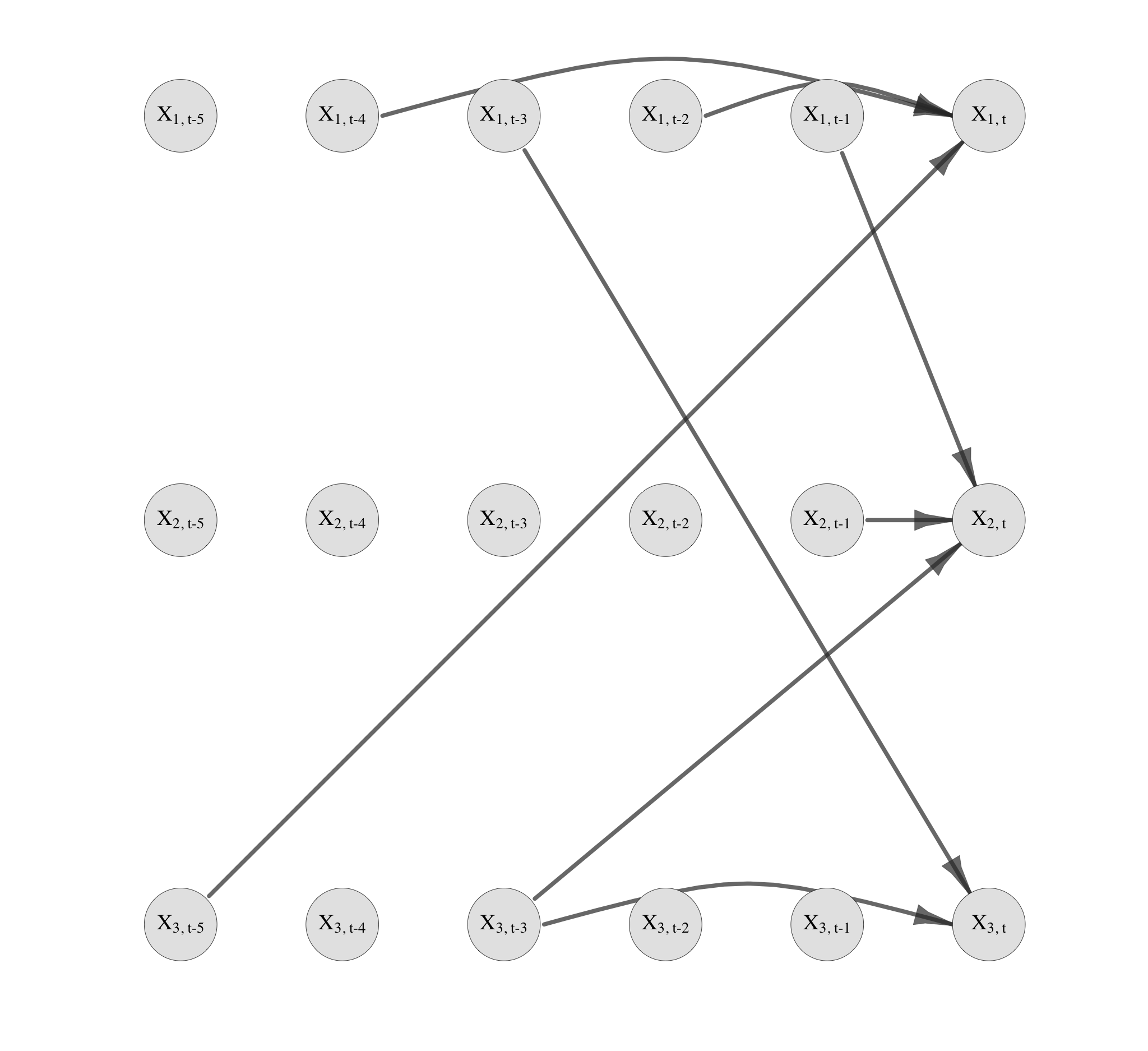
Refer to caption — Figure 1: A time-invariant DAG without instantaneous effects which corresponds to the SEM: $X_{1,t}=0.8X_{1,t-2}-0.3X_{1,t-4}+0.5X_{3,t-5}+\epsilon_{1,t}$ , $X_{2,t}=-0.7X_{1,t-1}+\sqrt{|X_{2,t-1}+X_{3,t-3}|}+\epsilon_{2,t}$ and $X_{3,t}=\sin(X_{1,t-3}X_{3,t-3})+\epsilon_{3,t}$ . The nodes correspond to variables $\{X_{c,t};\ c=1,\ldots,l;\ t\in\mathbb{Z}\}$ . Due to stationarity and the Markovian structure, it is sufficient to represent the DAG for time points $t,\ldots,t-p_{0}$ .

We denote the causal effect at $X_{c_{1},t}$ after an intervention at $X_{c_{2},t-s},\,s\in\mathbb{N}$ by $\mathbb{E}[X_{c_{1},t}\,|\,\mathrm{do}(X_{c_{2},t-s}$
$=x)]$ , where $c_{1},\,c_{2}$ are components of the multivariate time series. Also, $t$ is the time index of the response variable and $s$ the time difference between intervention and response variable. Let $\mathbf{X}_{1},\ldots,\mathbf{X}_{n}$ be a sample of the sequence. We estimate the causal effect as

\hat{\mathbb{E}}[X_{c_{1},t}\,|\,\mathrm{do}(X_{c_{2},t-s}=x)]=(n-s-p)^{-1}\sum_{k=s+p+1}^{n}\hat{m}(x,\mathbf{X}_{k-s}^{\mathcal{S}}),

(7)

where $\mathbf{X}_{t}^{\mathcal{S}}$ denotes the set $\{\mathbf{X}_{t-1},\ldots,\mathbf{X}_{t-p}\}$ with $p\geq p_{0}$ chosen reasonably large such that it is larger than the Markovian order $p_{0}$ . The partially locally linear estimator $\hat{m}(x,\mathbf{x}^{\mathcal{S}})$ is obtained by minimising

\sum_{k=s+p+1}^{n}(X_{c_{1},k}-\alpha-\beta(X_{c_{2},k-s}-x))^{2}K_{h_{1}}(X_{c_{2},k-s}-x)L_{h_{2}}(\mathbf{X}_{k-s}^{\mathcal{S}}-\mathbf{x}^{\mathcal{S}})

(8)

with respect to $\alpha$ and $\beta$ . We then use $\hat{m}(x,\mathbf{x}^{\mathcal{S}})=\hat{\alpha}$ . $K$ , $L$ are two kernel functions and $h_{1}$ , $h_{2}$ are their corresponding bandwidths. When the bandwidths are chosen appropriately, we are able to show that our estimator recovers the true causal effect consistently and with convergence rate $n^{-2/5}$ . For this purpose, we require some assumptions outlined next.

2.2 Asymptotic result

We assume the following conditions.

Assumption 1.

1.

The mixing coefficients of the underlying strongly mixing stationary $l$ -dimensional Markovian process of order $p_{0}$ satisfy $\alpha_{k}\leq Ak^{-\beta}$ and $\beta>2+\frac{pl+1}{\gamma}+pl$ for some constants $A>0$ , $\gamma>0$ and $p\geq p_{0}$ .
2.

The variables $X_{c,t}$ have bounded support for every $t\in\mathbb{Z}$ and $c\in\{1,\ldots,l\}$ .

The variables $X_{c_{2},t},\mathbf{X}_{t}^{\mathcal{S}}$ have a joint density with respect to Lebesgue measure and $p(u,\mathbf{u}^{\mathcal{S}})$ has continuous, bounded partial derivatives up to order 2 with respect to $u$ and up to order $d$ with respect to $\mathbf{u}^{\mathcal{S}}$ . In addition, for a $\delta>0$ the joint distribution is bounded away from zero in a neighbourhood of $x$

\underset{\mathbf{u}^{\mathcal{S}}\in\mathrm{supp}(\mathbf{X}_{t}^{\mathcal{S}})}{\underset{u\in x\pm\delta}{\inf}}p(u,\mathbf{u}^{\mathcal{S}})>0.

4.

The conditional density $p(\mathbf{X}_{i}^{\mathcal{S}}\,|\,\mathbf{X}_{j},\mathbf{X}_{j}^{\mathcal{S}},\mathbf{X}_{k},\mathbf{X}_{k}^{\mathcal{S}},\mathbf{X}_{l},\mathbf{X}_{l}^{\mathcal{S}})$ is bounded a.s. for every $i,j,k,l\in\mathbb{Z}$ .
5.

For every $j\in\mathbb{Z}$ the joint density $p(\mathbf{X}_{t},\mathbf{X}_{t}^{\mathcal{S}},\mathbf{X}_{t+j},\mathbf{X}_{t+j}^{\mathcal{S}})$ is bounded.
6.

The regression function $m(u,\mathbf{u}^{\mathcal{S}})=\mathbb{E}{[X_{c_{1},t}\,|\,X_{c_{2},t-s}=u,\mathbf{X}_{t-s}^{\mathcal{S}}=\mathbf{u}^{\mathcal{S}}]}$ exists and has bounded partial derivatives up to order 2 with respect to $u$ and up to order $d$ with respect to $\mathbf{u}^{\mathcal{S}}$ . Furthermore, $\mathbb{E}{[|X_{c_{1},t}|\,|\,X_{c_{2},t-s}=u,\mathbf{X}_{t-s}^{\mathcal{S}}=\mathbf{u}^{\mathcal{S}}]}$ is bounded.
7.

The kernel functions $K,L$ are symmetric, bounded on a bounded support and $L$ is an order $d$ -kernel.
8.

The product kernel $K\cdot L$ is Lipschitz, i.e., there exists a constant $\Lambda\geq 0$ such that for all $(u,v)$ and $(u^{\prime},v^{\prime})$

$|K(u)L(v)-K(u^{\prime})L(v^{\prime})|\leq\Lambda\|(u,v)-(u^{\prime},v^{\prime})\|\,.$
9.

The bandwidths are chosen such that $nh_{1}h_{2}^{2pl}/log^{2}(n)\rightarrow\infty$ and $h_{1}^{4}log(n)/h_{2}^{pl}\rightarrow 0$ , $h_{2}^{d}/h_{1}^{2}\rightarrow 0$ , $n^{\theta}h_{1}h_{2}^{pl}/log(n)\rightarrow\infty$ with $\theta=\frac{\beta-2-pl-(pl+1)/\gamma}{\beta+2-pl}$ .

Assumptions 1.2 - 1.3, 1.6 and the bandwidth conditions in 1.9 are adapted from Assumption 1 in [6]. Assumptions 1.1, 1.5, 1.7 - 1.9 ensure the uniform convergence of the kernel density estimator for dependent variables. In particular, a mixing rate is defined in Assumption 1.1 which yields the desired rate of convergence of the kernel density estimator.

Theorem 1.

Let $(\mathbf{X}_{t})_{t\in\mathbb{Z}}$ be a strictly stationary, strongly mixing Markovian process of order $p_{0}$ , and assume that it can be uniquely represented in the form of a structural equation model with time invariant DAG as in (6) which exhibits no instantaneous effects. Under Assumption 1, it holds that

\hat{\mathbb{E}}[X_{c_{1},t}\,|\,\mathrm{do}(X_{c_{2},t-s}=x)]-\mathbb{E}[X_{c_{1},t}\,|\,\mathrm{do}(X_{c_{2},t-s}=x)]=O(h_{1}^{2})+O_{p}(1/\sqrt{nh_{1}}).

Remark 1.

The rate $O(n^{-2/5})$ can be obtained by choosing $h_{1}\asymp n^{-1/5}$ if $pl<d$ . This corresponds to the optimal rate of convergence for the estimation of one-dimensional twice differentiable functions.

Remark 2.

Theorem 1 extends to the estimation of $\mathbb{E}[g(X_{c_{1},t})\,|\,\mathrm{do}(X_{c_{2},t-s}=x)]$ for arbitrary real-valued transformations $g(\cdot)$ (see Remark 1 [6]). For example, this enables the estimation of $\mathbb{E}[X_{c_{1},t}^{2}\,|\,\mathrm{do}(X_{c_{2},t-s}=x)]$ , $\mathbb{E}[|X_{c_{1},t}|\,|\,\mathrm{do}(X_{c_{2},t-s}=x)]$ or $P(X_{c_{1},t}\leq b\,|\,\mathrm{do}(X_{c_{2},t-s}=x))$ . This is especially useful in the analysis of financial time series. Financial returns often show no evidence of serial correlation, whereas the absolute returns or the squared returns do.

We defer the proof of Theorem 1 to A. The proof is a non-trivial extension of the techniques in Fan et al. [8] to the case of stationary Markovian processes. Alternatively, Theorem 1 might be derived by generalizing the theory of projections in Masry and Tjøstheim [17] to a fully nonparametric model with more than two projection components.

Furthermore, Hengartner and Sperlich [11] propose an interesting modification to the marginal integration estimator presented here. They suggest an internally normalised pilot estimator for the conditional mean which leads to nicer asymptotic results. Related to their motivation, we will discuss ways to ease the bandwidth choice and to bypass the use of higher order kernels for MINT-T in practice in the upcoming Sections 3 and 4.2.1.

2.3 Instantaneous effects

Up till now, we assumed that there are no instantaneous effects between the different components of the time series. Here, we will argue that some statements are still possible in presence of instantaneous effects while requiring no knowledge of the underlying DAG in the structural equation model (SEM). Instead of (6) we consider a SEM with DAG $D$

	$\displaystyle X_{c,t}=f_{c}(X_{\mathrm{pa}(c,t)},\epsilon_{c,t}),\ c=1,\ldots,l,\ t\in\mathbb{Z},$
	$\displaystyle\epsilon_{1,t},\ldots,\epsilon_{l,t}\ \mbox{jointly independent for all}\ t\in\mathbb{Z},$		(9)

where $\mathrm{pa}(c,t)$ is also allowed to include indices $(d,t)$ for some $d\neq c$ , i.e., so-called instantaneous effects (in Figure 1, there would be some directed edges among the variables $X_{1,t},\ldots,X_{l,t}$ ); and $\mathrm{pa}(c,t)$ is defined with respect to the DAG $D$ .

To deal with instantaneous effects, we have to choose another adjustment set. Ideally, when doing an intervention $\mathrm{do}(X_{c_{2},t-s}=x)$ we would choose an adjustment set like $\mathrm{pa}(c_{2},t-s)$ or a slightly larger set containing only ancestors of $(c_{2},t-s)$ . In absence of knowing the true underlying DAG, we cannot do this. We propose the following adjustment set

\displaystyle X_{c_{2},t-s}^{\tilde{\mathcal{S}}}:=\cup_{c\neq c_{2}}\{X_{c,t-s}\}\cup\{\mathbf{X}_{t-s-1},\ldots,\mathbf{X}_{t-s-p}\}

(10)

where $p\geq p_{0}$ . That is, we also include all instantaneous variables $X_{c,t-s}\ (c\neq c_{2})$ . The estimator is the same as in (7) but now using the larger adjustment set in (10). Using the theory as presented in Section 2.2, the estimator will converge, with rate $n^{-2/5}$ , to

\displaystyle\tilde{\mathbb{E}}[X_{c_{1},t}\,|\,\mathrm{do}(X_{c_{2},t-s}=x)]:=\int\mathbb{E}[X_{c_{1},t}\,|\,X_{c_{2},t-s}=x,X_{c_{2},t-s}^{\tilde{\mathcal{S}}}]dP(X_{c_{2},t-s}^{\tilde{\mathcal{S}}}).

In general, it will happen that

\displaystyle\tilde{\mathbb{E}}[X_{c_{1},t}\,|\,\mathrm{do}(X_{c_{2},t-s}=x)]\neq\mathbb{E}[X_{c_{1},t}\,|\,\mathrm{do}(X_{c_{2},t-s}=x)].

What we will argue though is that when $\tilde{\mathbb{E}}[X_{c_{1},t}\,|\,\mathrm{do}(X_{c_{2},t-s}=x)]\neq\mathbb{E}[X_{c_{1},t}]$ (and its estimate being sufficiently far away from the mean), one can claim a total causal effect of $X_{c_{2},t-s}$ on $X_{c_{1},t}$ . For a rigorous statement, we need the following definition.

Definition 1.

$X_{c_{2},t-s}$ is not total causal for $X_{c_{1},t}$ if and only if $X_{c_{2},t-s}\perp X_{c_{1},t}$ under the interventional distribution $P^{\mathbf{X}_{t}|\mathrm{do}(X_{c_{2},t-s}=x)}$ for all $x\in\mathrm{supp}(X_{c_{2},t-s})$ . Here, ” $\perp$ ” denotes independence.

Apparently, if $X_{c_{2},t-s}$ is not total causal for $X_{c_{1},t}$ , then the average causal effect $\mathbb{E}[X_{c_{1},t}\,|\,\mathrm{do}(X_{c_{2},t-s}$
$=x)]\equiv\mathbb{E}[X_{c_{1},t}]$ . We will show next that the same holds true for $\tilde{\mathbb{E}}[X_{c_{1},t}\,|\,\mathrm{do}(X_{c_{2},t-s}=x)]$ .

Theorem 2.

Let $(\mathbf{X}_{t})_{t\in\mathbb{Z}}$ be a strictly stationary Markovian process of order $p_{0}$ , and assume that it is represented in the form of a structural equation model with time invariant DAG $D$ as in (9) allowing also for instantaneous effects. Assume that, for all $x\in\mathrm{supp}(X_{c_{2},t-s})$ , the interventional distribution $P^{\mathbf{X}_{t}|\mathrm{do}(X_{c_{2},t-s}=x)}$ after the intervention $\mathrm{do}(X_{c_{2},t-s}=x)$ is faithful with respect to the interventional DAG $D_{\mathrm{interv}}$ where all directed arrows into $(c_{2},t-s)$ are deleted. Then from $\tilde{\mathbb{E}}[X_{c_{1},t}\,|\,\mathrm{do}(X_{c_{2},t-s}=x)]\neq\mathbb{E}[X_{c_{1},t}]$ for some $x\in\mathrm{supp}(X_{c_{2},t})$ , it follows that $X_{c_{2},t-s}$ is total causal for $X_{c_{1},t}$ for $s>0$ .

Remark 3.

The distribution of the stochastic process does not necessarily define a unique DAG. We note that the statement is true for any DAG $D$ such that the faithfulness and the Markov property hold.

Remark 4.

If we know beforehand that we are only interested in a set of prespecified intervention values $\mathcal{I}\subset\mathrm{supp}(X_{c_{2},t-s})$ , then the above assumption ” $P^{\mathbf{X}_{t}|\mathrm{do}(X_{c_{2},t-s}=x)}$ is faithful with respect to $D_{\mathrm{interv}}$ for all $x\in\mathrm{supp}(X_{c_{2},t-s})$ ” can be weakened to require only ”for all $x\in\mathcal{I}$ ”. The statement of the theorem then reads: from $\tilde{\mathbb{E}}[X_{c_{1},t}\,|\,\mathrm{do}(X_{c_{2},t-s}=x)]\neq\mathbb{E}[X_{c_{1},t}]$ for some $x\in\mathcal{I}$ , it follows that $X_{c_{2},t-s}$ is total causal for $X_{c_{1},t}$ for $s>0$ .

Just as in Theorem 1, we are able to estimate $\tilde{\mathbb{E}}[X_{c_{1},t}\,|\,\mathrm{do}(X_{c_{2},t-s}=x)]$ with the optimal rate by adjusting on $X_{c_{2},t-s}^{\tilde{\mathcal{S}}}$ from (10) in the presence of instantaneous effects. Thus, if $\widehat{\tilde{\mathbb{E}}}[X_{c_{1},t}\,|\,\mathrm{do}(X_{c_{2},t-s}=x)]\neq\overline{X}_{c_{1},.}$ , we would claim a total causal effect and hence avoid false positive statements about causal effects. A word of caution should be added, however: we would typically rank different causal effects by a quantity like

\displaystyle\mathrm{eff}\left(X_{c_{2},t-s}\to X_{c_{1},t}\right)=\int\|\mathbb{E}[X_{c_{1},t}\,|\,\mathrm{do}(X_{c_{2},t-s}=x)]-\mathbb{E}[X_{c_{1},t}]\|dw(x)

for some weight function $w(\cdot)$ . This causal effect quantity can be rather different from

\displaystyle\widetilde{\mathrm{eff}}\left(X_{c_{2},t-s}\to X_{c_{1},t}\right)=\int\|\tilde{\mathbb{E}}[X_{c_{1},t}\,|\,\mathrm{do}(X_{c_{2},t-s}=x)]-\mathbb{E}[X_{c_{1},t}]\|dw(x).

Thus, a ranking of total causal effects by estimates of $\widetilde{\mathrm{eff}}(\cdot)$ can be rather different than by estimates of the true causal effects $\mathrm{eff}(\cdot)$ .

Proof of Theorem 2.

To simplify notation and without loss of generality assume that $\mathbb{E}[X_{c,t}]=0$ for all $c$ . We will show the reverse implication: $X_{c_{2},t-s}$ is not total causal for $X_{c_{1},t}\Rightarrow\tilde{\mathbb{E}}[X_{c_{1},t}\,|\,\mathrm{do}(X_{c_{2},t-s}$
$=x)]\equiv 0$ . If $X_{c_{2},t-s}$ is not total causal for $X_{c_{1},t}$ , $X_{c_{1},t}$ and $X_{c_{2},t-s}$ are independent under the interventional distribution $P^{\mathbf{X}_{t}|\mathrm{do}(X_{c_{2},t-s}=x)}$ for all $x\in\mathrm{supp}(X_{c_{2},t-s})$ . On a graphical level, the intervention $\mathrm{do}(X_{c_{2},t-s}=x)$ corresponds to deleting all incoming edges into $(c_{2},t-s)$ from the observational DAG $D$ and substituting $X_{c_{2},t-s}$ by $x$ in the resulting interventional DAG $D_{\mathrm{interv}}$ . The independence between $X_{c_{1},t}$ and $X_{c_{2},t-s}$ can be translated into a graphical criterion, namely that $X_{c_{1},t}$ and $X_{c_{2},t-s}$ are d-seperated by the empty set in $D_{\mathrm{interv}}$ to which $P^{\mathbf{X}_{t}|\mathrm{do}(X_{c_{2},t-s}=x)}$ is faithful for all $x$ . Then, there can only be paths between $X_{c_{2},t-s}$ and $X_{c_{1},t}$ that contain at least one v-structure. We denote such a v-structure by $X_{c_{\mathrm{source}_{1}},t-j_{1}}\rightarrow X_{c_{\mathrm{collider}},t-j_{2}}\leftarrow X_{c_{\mathrm{source_{2}}},t-j_{3}}$ . Here, $c_{\mathrm{source}_{1}}$ or $c_{\mathrm{source}_{2}}$ could be equal to $c_{\mathrm{collider}}$ but not both.

If the collider $X_{c_{\mathrm{collider}},t-j_{2}}$ lies between $j_{2}=0,..,s-1$ , nothing changes by adjusting on $X_{c_{2},t-s}^{\tilde{\mathcal{S}}}$ . The path still remains blocked by $X_{c_{\mathrm{collider}},t-j_{2}}$ . On the other hand, if $j_{2}=s$ , then $j_{1},j_{3}\geq s$ and the path is blocked by either $X_{c_{\mathrm{source}_{1}},t-j_{1}}$ or $X_{c_{\mathrm{source}_{2}},t-j_{3}}$ after adjusting on $X_{c_{2},t-s}^{\tilde{\mathcal{S}}}$ . Therefore, every path between $X_{c_{1},t}$ and $X_{c_{2},t-s}$ is blocked by $X_{c_{2},t-s}^{\tilde{\mathcal{S}}}$ in $D_{\mathrm{interv}}$ .

Since $P$ is Markov w.r.t. $D$ , we have conditional independence of $X_{c_{1},t}$ and $X_{c_{2},t-s}$ given $X_{c_{2},t-s}^{\tilde{\mathcal{S}}}$ and therefore,

			$\displaystyle\tilde{\mathbb{E}}[X_{c_{1},t}\,\|\,\mathrm{do}(X_{c_{2},t-s}=x)]=\int\mathbb{E}[X_{c_{1},t}\,\|\,X_{c_{2},t-s}=x,X_{c_{2},t-s}^{\tilde{\mathcal{S}}}]dP(X_{c_{2},t-s}^{\tilde{\mathcal{S}}})$
		$\displaystyle=$	$\displaystyle\int\mathbb{E}[X_{c_{1},t}\,\|\,X_{c_{2},t-s}^{\tilde{\mathcal{S}}}]dP(X_{c_{2},t-s}^{\tilde{\mathcal{S}}})=\mathbb{E}[X_{c_{1},t}]=0.$

∎

3 Implementation

The estimator in (7) is constructed using the partially locally linear estimator in (8). This requires choosing two bandwidths $h_{1}$ and $h_{2}$ , and such a choice is not easy in view of the fact that we cannot rely on cross-validation for the quantity $\mathbb{E}[X_{c_{1},t}\,|\,\mathrm{do}(X_{c_{2},t-s}=x)]$ (since there is no corresponding loss to an observable quantity). The related estimator suggested by [6], based on a boosting idea, seems substantially easier for practical purposes.

3.1 MINT-T: an implementation for marginal integration

We describe here our estimation scheme based on the boosting idea in [6]: we call it ”MINT-T”, standing for marginal integration in time series. MINT-T differs from the estimation scheme in [6] in that no additive approximation is used in the first step. The more regular structure of our setting (e.g., stationarity assumption, same size of adjustment set for all interventions) allows us to directly apply the marginal integration estimator from the first step.

Exploiting the strict stationarity of the time series, we obtain $n-s-p$ dependent samples (i.e., samples of ”regressors”). For $X_{c_{1},t}$ and $X_{c_{2},t-s}$ , we have the ”response” vector $\mathbb{X}_{c_{1}}:=\{X_{c_{1},n},X_{c_{1},n-1},\ldots,X_{c_{1},s+p+1}\}$ and the ”regressor” $\mathbb{X}_{c_{2}}:=\{X_{c_{2},n-s},X_{c_{2},n-s-1},\ldots,X_{c_{2},p+1}\}$ , respectively. For the adjustment set $\textbf{X}^{\mathcal{S}}_{t-s}$ , we have the lagged values of the ”regressors” which can be represented by the matrix $(\textbf{X}_{n-s-1}(p),\ldots,\textbf{X}_{p}(p))$ , where $\textbf{X}_{t}(p)=(\textbf{X}_{t},\ldots,\textbf{X}_{t-p+1})$ . This matrix involves the samples $\mathbb{X}^{\mathcal{S}}:=\{\textbf{X}_{n-s-1},\ldots,\textbf{X}_{1}\}$ .

The initial step of MINT-T consists of approximating the regression function $m(x,\textbf{x}^{\mathcal{S}})=\mathbb{E}[X_{c_{1},t}\mid X_{c_{2},t-s}=x,\textbf{X}^{\mathcal{S}}_{t-s}=\textbf{x}^{\mathcal{S}}]$ by a locally constant estimator of the form

\hat{m}_{\text{init}}(x,\textbf{x}^{\mathcal{S}}):=\operatornamewithlimits{argmin}\limits_{\alpha}\sum\limits_{k=s+p+1}^{n}(X_{c_{1},k}-\alpha)^{2}K_{h_{1}}(X_{c_{2},k-s}-x)L_{h_{2}}(\textbf{X}^{\mathcal{S}}_{k-s}-\textbf{x}^{\mathcal{S}}).

(11)

Marginally integrating the estimator (11) over the samples $\mathbb{X}^{\mathcal{S}}$ with the empirical mean as in equation (8) yields an estimate for the true causal effect $\mathbb{E}[X_{c_{1},t}\,|\,\mathrm{do}(X_{c_{2},t-s}=x)]$ . The problem is that the marginally integrated estimator (8) is very sensitive to the choice of the bandwidths $h_{1}$ and $h_{2}$ . Moreover, we cannot use cross-validation or penalised likelihood techniques to determine the optimal bandwidths as $\mathbb{E}[X_{c_{1},t}\,|\,\mathrm{do}(X_{c_{2},t-s}=x)]$ is neither a regression function nor does it appear in the likelihood. To make our estimator more robust with respect to the choice of the bandwidths, we therefore apply $B$ steps of $L_{2}$ -boosting with the locally constant estimator (11), which, in every iteration, is applied to the residuals of the previous fit. The key idea of the boosting procedure is that the bandwidths $h_{1}$ and $h_{2}$ in (11) can be set to large values in order to obtain an estimator with high bias and low variance. The boosting iterations then reduce the bias. As such, the boosted estimator is less sensitive to the specific choice of the bandwidths as long as they are sufficiently large. This will be shown experimentally in Section 4.2.1. The effect of the boosting can be compared to the one of the use of a higher-order kernel [5].

We now describe the boosting procedure in detail. Let $\hat{m}_{1}:=\hat{m}_{\text{init}}$ defined in (11). Then, the $n-s-p$ residuals $R_{1,s+p+1},\ldots,R_{1,n}$ of the initial model fit are given as

R_{1,k}=X_{c_{1},k}-\hat{m}_{1}(X_{c_{2},k-s},\textbf{X}^{\mathcal{S}}_{k-s}),\qquad k=s+p+1,\ldots,n.

The locally constant fit of the residuals is then obtained as in (11) by minimising

\sum\limits_{k=s+p+1}^{n}(R_{1,k}-\alpha)^{2}K_{h_{1}}(X_{c_{2},k-s}-x)L_{h_{2}}(\textbf{X}^{\mathcal{S}}_{k-s}-\textbf{x}^{\mathcal{S}})

(12)

with respect to $\alpha$ , and is denoted by $\hat{g}_{R_{1}}(x,\textbf{x}^{\mathcal{S}}):=\hat{\alpha}$ . Let $\hat{\textbf{m}}$ be the $(n-s-p)$ -dimensional vector of $\hat{m}$ evaluated at the samples of the time series and $\textbf{X}_{c_{1}}$ be the $(n-s-p)$ -dimensional vector of the samples in $\mathbb{X}_{c_{1}}$ . We can then summarise the $L_{2}$ -boosting step as follows: for $b=1,\ldots,B-1$ ,

	$\displaystyle\hat{m}_{b+1}$	$\displaystyle=\hat{m}_{b}+\hat{g}_{R_{b}},$
	$\displaystyle\textbf{R}_{b+1}$	$\displaystyle=\textbf{X}_{c_{1}}-\hat{\textbf{m}}_{b+1},$

where $B$ (the number of boosting iterations) is a regularisation parameter.

Finally, we marginally integrate over the samples $\mathbb{X}^{\mathcal{S}}$ with the empirical mean. This last step of MINT-T yields the final estimate

\hat{\mathbb{E}}[X_{c_{1},t}\mid\mathrm{do}(X_{c_{2},t-s}=x)]=(n-s-p)^{-1}\sum\limits_{k=s+p+1}^{n}\hat{m}_{B}(x,\textbf{X}_{k-s}^{\mathcal{S}}).

The pseudo-code summarising our method is provided in Algorithm 1.

1: Construct

n-s-p

samples of the adjustment set, the intervention variable and the target variable exploiting the strict stationarity of the time series.

2: Fit an initial locally constant estimator of

X_{c_{1},t}

versus

X_{c_{2},t}

and

\textbf{X}^{\mathcal{S}}_{t-s}

with large bandwidths to obtain

\hat{m}_{1}:=\hat{m}_{\text{init}}

in (11).

3: for

b=1,\ldots,B-1

4: Apply one step of

L_{2}

-boosting as follows:

5: (i) Compute residuals

\textbf{R}_{b}=\textbf{X}_{c_{1}}-\hat{\textbf{m}}_{b}

6: (ii) Fit the residuals with the kernel estimator (12) to obtain

\hat{g}_{R_{b}}

7: (iii) Set

\hat{m}_{b+1}=\hat{m}_{b}+\hat{g}_{R_{b}}

8: end for

9: return Do marginal integration: output

(n-s-p)^{-1}\sum\limits_{k=s+p+1}^{n}\hat{m}_{B}(x,\textbf{X}^{\mathcal{S}}_{k-s})

Algorithm 1 MINT-T

4 Empirical results

We provide here empirical results of the marginal integration method MINT-T for the estimation of causal effects. We also compare it to a reference method, explained below, which relies on approximating the data-generating stochastic process. This is of course a very ambitious task and, in its full generality, exposed to the curse of dimensionality.

4.1 A reference method

For comparison, we consider a reference method where we assume that the time series has an additive functional form with an additive Gaussian error term. This assumption may easily fail though and thus, the method is exposed to model misspecification. We then estimate the value of each of the $l$ components of $\textbf{X}_{t}$ by an additive function of the $p$ previous values of all components, that is,

$\displaystyle X_{1,t}$	$\displaystyle=\hat{\mu}^{(1)}+\sum\limits_{c=1}^{l}\sum\limits_{j=1}^{p}\hat{m}^{(1)}_{c,t-j}(X_{c,t-j})+\hat{\epsilon}_{1,t}$
	$\displaystyle\ \ \vdots$	(13)
$\displaystyle X_{l,t}$	$\displaystyle=\hat{\mu}^{(l)}+\sum\limits_{c=1}^{l}\sum\limits_{j=1}^{p}\hat{m}^{(l)}_{c,t-j}(X_{c,t-j})+\hat{\epsilon}_{l,t}.$

We now set $X_{1,j}=X_{2,j}=,\ldots,=X_{l,j}=0$ for $j=1,\ldots,p$ and then iteratively simulate the subsequent values at time points $p+1,p+2,\ldots,n$ of the time series using the estimated functions and estimated error terms from the additive model (13) with one exception: when reaching time point $n-s$ , we intervene on component $c_{2}$ by setting $X_{c_{2},n-s}$ to the value $x$ . In the end, we record the simulated value $\hat{X}_{c_{1},n}$ . We repeat the whole procedure $N$ times to obtain $N$ simulated realizations $\{\hat{X}_{c_{1},n}^{(1)},\ldots,\hat{X}_{c_{1},n}^{(N)}\}$ . For sufficiently large $N$ , the total causal effect at $X_{c_{1},t}$ after an intervention at $X_{c_{2},t-s}$ can be estimated as

\hat{\mathbb{E}}[X_{c_{1},t}\mid\mathrm{do}(X_{c_{2},t-s}=x)]=N^{-1}\sum\limits_{i=1}^{N}\hat{X}_{c_{1},n}^{(i)}.

4.1.1 Approximating the true causal effect

If the functional form of the true underlying time series and the distributions of the error terms are known, we can use the reference method for computing the true causal effect. We then simply replace the estimated functions and noise variables in the additive model (13) by the (not necessarily additive) true ones, but apart from that stick to the simulation procedure described above.

4.2 Simulations

We examine here MINT-T on simulated time series from a variety of models covering linear to nonlinear, additive to non-additive, and univariate to multivariate models:

•

Model 1: $X_{t}=0.4X_{t-2}-0.6X_{t-6}+0.3X_{t-10}+\epsilon_{t}$
•

Model 2: $X_{t}=\cos(X_{t-1}+X_{t-4})+\log(|X_{t-6}-X_{t-10}|+1)+\epsilon_{t}$
•

Model 3: $X_{t}=\sigma_{t}\epsilon_{t}$ with $\sigma_{t}^{2}=0.1+0.4X_{t-1}^{2}+0.2X_{t-4}^{2}$
•

Model 4: $X_{t}=\sigma_{t}\epsilon_{t}$ with $\sigma_{t}^{2}=0.2+0.6X_{t-1}^{2}+0.3\sigma_{t-1}^{2}$
•

Model 5: $X_{t}=0.4X_{t-1}-0.2X_{t-2}+0.3X_{t-3}+0.8\epsilon_{t-1}+\epsilon_{t}$
•

Model 6: $\left(\begin{array}[]{c}X_{1,t}\\ X_{2,t}\\ X_{3,t}\\ X_{4,t}\end{array}\right)=\left(\begin{array}[]{l}0.4X_{1,t-1}-0.2X_{1,t-2}+0.3X_{2,t-3}+\epsilon_{1,t}\\ \cos(X_{1,t-1})+\log(|X_{2,t-2}|+1)+\epsilon_{2,t}\\ \sin(X_{3,t-1}-X_{2,t-1})+\sqrt{|X_{2,t-3}+X_{4,t-1}|}+\epsilon_{3,t}\\ \cos(X_{2,t-1}-X_{3,t-4})+\log(|X_{1,t-6}+X_{2,t-10}|+1)+\epsilon_{4,t}\end{array}\right)$

The first model is a linear $\mathrm{AR}(10)$ and model 2 a nonlinear, non-additive $\mathrm{AR}(10)$ -model. The third model corresponds to an $\mathrm{ARCH}(4)$ -model and the fourth model to a $\mathrm{GARCH}(1,1)$ -model. The fifth is an $\mathrm{ARMA}(3,2)$ -model and the last a multivariate time series model with four (additive and non-additive) components. In our simulation study we choose i.i.d. Gaussian noise with mean zero and variance 1 for models 1-3, 6 and variance 0.5 for models 4 and 5. In all our numerical experiments, we choose sample size $n=1000$ .

For each model, we inspect the mean squared error (MSE) between the true and the estimated causal effect. More precisely, the MSE consists of the true effect subtracted from the estimated causal effect averaged over 20 cause and effect pairs:

\frac{1}{20}\sum_{j=1}^{20}\sum_{i=1}^{9}(\hat{\mathbb{E}}[X_{t}|\mathrm{do}(X_{t-j}=d_{i})]-\mathbb{E}[X_{t}|\mathrm{do}(X_{t-j}=d_{i})])^{2}.

We employ the nine deciles $d_{1},\ldots,d_{9}$ of the simulated time series (quantiles corresponding to the probabilities $0.1,0.2,\ldots,0.9$ ) as the intervention values. For the multivariate model 6, we sample the components of the intervention and response variable uniformly, repeat the calculation over 5 repetitions and average over the resulting MSE values. Our method MINT-T requires the following tuning parameters: the bandwidths $h_{1}$ and $h_{2}$ , the time lag $p$ and the number of boosting iterations $B$ . We use the true time lag $p$ whenever it is known. This is mainly for comparison reason so that the reference method is not disadvantaged. For the non-Markovian models 4 and 5, we set $p$ to 10. The bandwidth $h_{1}$ is set to $2\hat{\sigma}$ for univariate and $3\hat{\sigma}_{c_{2}}$ for multivariate time series, where $\hat{\sigma}$ denotes the empirical standard deviation of the time series. We used a product Gaussian kernel for $L$ in equation (11). The bandwidth $h_{2}$ is a $p$ -dimensional vector for univariate time series and chosen as $(2\hat{\sigma},\ldots,2\hat{\sigma})$ due to stationarity, while for multivariate time series, $h_{2}$ is a $pl$ -dimensional vector and each entry is scaled by the standard deviation of the corresponding component, i.e., $(3\hat{\sigma}_{1},\ldots,3\hat{\sigma}_{l},\ldots,3\hat{\sigma}_{1},\ldots,3\hat{\sigma}_{l})$ . In the univariate case, $h_{1}$ and each element from $h_{2}$ are equal. For simplicity and with slight abuse of notation, we refer to both $h_{1}$ and each entry of $h_{2}$ as $h$ , where for the multivariate case we actually mean that the bandwidth is scaled by the corresponding standard deviation of the component. The number of boosting iterations $B$ is set to 10. The exact choices of $h$ , $B$ are not crucial as long as both parameters are chosen reasonably large. Moreover, our estimator is rather insensitive to the choice of $p$ . This will be explained in more detail in Sections 4.2.1 and 4.2.2. For the reference method we simulated 1000 and for the true causal effect we simulated 10000 time series for every intervention variable and intervention value.

The experimental findings are summarised in Table 1. The relative gain is calculated from the formula $(\text{MSE}_{\mathrm{reference}}-\text{MSE}_{\mathrm{MINT-T}})/\text{MSE}_{\mathrm{reference}}$ and the acceleration factor from $\text{time}_{\mathrm{reference}}/\text{time}_{\mathrm{MINT-T}}$ . Our empirical results show that MINT-T outperforms the reference procedure on all models except for the univariate $\mathrm{AR}$ -models (model 1 and 2). In theory, we expect the reference to have an advantage when the underlying model is additive, as it is the case with model 1. Even though model 2 is a nonlinear $\mathrm{AR}$ -model, our results show that it can be well approximated through additive modelling. MINT-T is able to provide a relative gain of 17 $\%$ -53 $\%$ over the reference on the $\mathrm{ARCH}$ -, $\mathrm{GARCH}$ -, $\mathrm{ARMA}$ - and the multivariate model.

In some situations, it is of interest to choose intervention values that lie outside of the range of the time series. In Table 2, we set the intervention value $d_{i}$ to 3 times the $i^{th}$ decile of the simulated time series. As a result, the range of the simulated true causal effects becomes larger, and the MSE of both methods increases. In comparison, MINT-T remains more robust for intervention values that lie outside of the range of the data points and achieves a relative gain of at least 45 $\%$ on all models.

	MSE			Time $[s]$			True effect
	MINT-T	Reference	Gain/loss	MINT-T	Reference	Accel.	between
Model 1	0.0804	0.0682	-17.89%	16.17	880.15	54	[-0.6355,0.5645]
Model 2	0.0459	0.0291	-57.73 %	16.26	922.38	57	[0.4408,1.2937]
Model 3	0.0026	0.0046	+43.48%	8.48	419.74	49	0
Model 4	0.0014	0.0027	+48.15%	17.14	938.65	55	0
Model 5	0.0333	0.0711	+53.16%	17.17	946.76	55	[-0.381, 0.3267]
Model 6	0.1430	0.1724	+17.05%	58.18	14788.29	254	[0.3114, 1.9647]

Table 1: Comparison of MINT-T against the reference in terms of MSE and CPU time consumption per index pair. Relative gain (indicated by +) and loss (indicated by -), and acceleration factor for the CPU time.

	MSE			Time $[s]$			True effect
	MINT-T	Reference	Gain/loss	MINT-T	Reference	Accel.	between
Model 1	0.1791	0.5176	+65.40%	21.26	1036.13	49	[-1.9433,1.6647]
Model 2	0.4688	1.2139	+61.38 %	33.85	2086.42	62	[ 0.4538,1.9718]
Model 3	0.0261	0.0475	+45.05%	11.76	523.72	45	0
Model 4	0.0079	0.0213	+62.91%	19.87	1064.73	54	0
Model 5	0.1081	0.4310	+74.92%	21.76	1021.42	47	[-1.1320, 0.9798]
Model 6	0.5919	2.6364	+77.55%	64.53	14506.34	225	[ 0.3090, 3.1312 ]

Table 2: Comparison of MINT-T against the reference in terms of MSE and CPU time consumption per index pair. Relative gain (indicated by +) and loss (indicated by -), and acceleration factor for the CPU time. Unlike Table 1 and 3, the intervention value

d_{i}

here is equal to 3 times the

i^{th}

decile of each time series.

In many applications, we are interested in the effect of an intervention on a transformed response variable. For example, any causal effect is identical to zero in $\mathrm{ARCH}$ -models since

$\displaystyle\mathbb{E}[X_{t}\,\|\,\mathrm{do}(X_{t-s}=x)]$	$\displaystyle=$	$\displaystyle\int\mathbb{E}[X_{t}\,\|\,X_{t-s}=x,X_{t-s}^{\mathcal{S}}]dP(X_{t-s}^{\mathcal{S}})$
	$\displaystyle=$	$\displaystyle\int\mathbb{E}[\sigma_{t}\epsilon_{t}\,\|\,X_{t-s}=x,X_{t-s}^{\mathcal{S}}]dP(X_{t-s}^{\mathcal{S}})$
	$\displaystyle=$	$\displaystyle\int\mathbb{E}[\sigma_{t}\,\|\,X_{t-s}=x,X_{t-s}^{\mathcal{S}}]\mathbb{E}[\epsilon_{t}]dP(X_{t-s}^{\mathcal{S}})=0.$

An intervention on a squared response variable is usually nonzero in $\mathrm{ARCH}$ -models and corresponds to an intervention on the volatility function up to a constant:

$\displaystyle\mathbb{E}[X_{t}^{2}\,\|\,\mathrm{do}(X_{t-s}=x)]$	$\displaystyle=$	$\displaystyle\int\mathbb{E}[X_{t}^{2}\,\|\,X_{t-s}=x,X_{t-s}^{\mathcal{S}}]dP(X_{t-s}^{\mathcal{S}})$
	$\displaystyle=$	$\displaystyle\int\mathbb{E}[\sigma_{t}^{2}\epsilon_{t}^{2}\,\|\,X_{t-s}=x,X_{t-s}^{\mathcal{S}}]dP(X_{t-s}^{\mathcal{S}})$
	$\displaystyle=$	$\displaystyle\int\mathbb{E}[\sigma_{t}^{2}\,\|\,X_{t-s}=x,X_{t-s}^{\mathcal{S}}]E[\epsilon_{t}^{2}]dP(X_{t-s}^{\mathcal{S}})$
	$\displaystyle=$	$\displaystyle\mathrm{Var}(\epsilon_{t})\mathbb{E}[\sigma_{t}^{2}\,\|\,\mathrm{do}(X_{t-s}=x)].$

	MSE			Time $[s]$			True effect
	MINT-T	Reference	Gain/loss	MINT-T	Reference	Accel.	between
Model 1	0.0297	0.0482	+38.38%	17.00	967.50	57	[1.1372,1.5856]
Model 2	0.1647	0.1746	+5.67%	17.49	957.27	55	[1.7211,3.2016]
Model 3	0.0026	0.0045	+42.22%	8.76	401.30	46	[0.1523,0.2924]
Model 4	0.0008	0.0009	+11.11%	17.12	930.56	54	[0.0502,0.0940]
Model 5	0.0125	0.0407	+69.29%	17.52	929.60	53	[0.3184,0.4700]
Model 6	1.1216	1.2232	+8.31 %	60.51	16051.16	265	[1.5119,5.4317]

Table 3: Comparison of MINT-T against the reference in terms of MSE and CPU time consumption per index pair for the squared response variable. Relative gain (indicated by +) and loss (indicated by -), and acceleration factor for the CPU time.

Similarly, stationary $\mathrm{GARCH}$ -processes can be rewritten as $\mathrm{ARCH}(\infty)$ processes, and the causal effect is identical to 0, while a squared $\mathrm{GARCH}$ -process can be rewritten as a causal and invertible $\mathrm{ARMA}$ -process under certain conditions [7, Proposition 4.2]. Our approach allows for the estimation of causal effects on transformed response variables with arbitrary real-valued transformations (see Remark 2). We repeat the analysis for a squared response variable, and the experimental results are listed in Table 3. MINT-T outperforms the reference on all models. The relative gain lies between 6 $\%$ on the nonlinear $\mathrm{AR}$ -model to 69 $\%$ on the $\mathrm{ARMA}$ -model.

Another advantage of MINT-T is the computation time. The computation time of MINT-T depends mainly on the size of the adjustment set and the number of boosting iterations. On the other hand, prediction and fitting of the generalised additive models require most of the computation time for the reference method. The reference method fits once and predicts once for every component at every time point. MINT-T provides an acceleration by a factor of 53, on average, for univariate and an acceleration by a factor of 248, on average, for multivariate time series. Therefore, MINT-T remains feasible for multivariate time series in potentially large-dimensional problems.

4.2.1 The choice of the bandwidth $h$

We tested different bandwidths $h$ in the range of $0.1\hat{\sigma}-10\hat{\sigma}$ for the simulated time series from Section 4. In Figures 2 and 3, the MSE values are plotted against $h$ . We observe that with no boosting, the performance is sensitive to the choice of the bandwidth. There is typically an optimal bandwidth if no boosting iterations are performed. For example, the optimal bandwidth is $h\approx 0.6\hat{\sigma}$ for model 1 and $h\approx 0.8\hat{\sigma}$ for model 5. The sensitivity largely disappears with increasing number of boosting iterations. Moreover, boosting is able to decrease the MSE. Therefore, we can simply take a larger bandwidth in connection with subsequent boosting. We suggest the following rule-of-thumb: $h=2\hat{\sigma}$ for univariate and $h=c_{l}\cdot 2\hat{\sigma}$ for multivariate time series along with $10$ boosting iterations. The factor $c_{l}$ is approximately equal to $n^{\frac{1}{4+p}-\frac{1}{4+pl}}$ and corrects for the dimensionality of the adjustment sets, i.e., $p$ for univariate and $pl$ for multivariate time series. For $n=1000$ , $l=4$ and $p=10$ , we used $c_{l}=1.5$ . The observed results are consistent with what we outlined in Section 3: it is favourable to choose large bandwidths, which results in an initial estimate with large bias and small variance, and the bias is subsequently reduced by the boosting iterations.

In order to avoid unnecessary boosting iterations or ”overboosting”, we implemented the following stopping rules, which are also shown in Figures 2 and 3. First, we sum the absolute differences between two consecutive approximations:

C(b):=\sum\limits_{i=1}^{9}|(n-s-p)^{-1}\sum\limits_{k=s+p+1}^{n}\hat{g}_{R_{b}}(d_{i},\textbf{X}_{k-s}^{\mathcal{S}})|.

(14)

Then we terminate the boosting iterations if either the absolute difference $C(b)$ is smaller than 0.5% of the previous estimate $\sum\limits_{i=1}^{9}|(n-s-p)^{-1}\sum\limits_{k=s+p+1}^{n}\hat{m}_{b}(d_{i},\textbf{X}_{k-s}^{\mathcal{S}})|$ or if the proportion of two subsequent differences $C(b)/C(b-1)$ is less than 75% (see Section 3). This way, we achieve little to no boosting for small bandwidths (small bias, high variance estimate) and more boosting iterations for larger bandwidths (high bias, small variance estimate). Apparently, our proposed stopping rule performs reasonably well in the univariate examples we considered. For multivariate time series, the percentages used for the stopping rule should be adapted to the dimension of the time series. Additional simulations for the remaining models are presented in Section B.1.

4.2.2 The choice of the time lag $p$ for adjustment

MINT-T requires an estimated time lag $p$ for the adjustment set indicated with $\mathcal{S}$ . We ran MINT-T on the simulated time series from Section 4 for different values of $p$ between 1 and 20. The corresponding MSE values for $h=0.6\hat{\sigma}$ , $h=2\hat{\sigma}$ and $h=4\hat{\sigma}$ are shown in Figure 4.

We observe in Figure 4 that for small bandwidths, e.g., $h=0.6\hat{\sigma}$ , the performance is sensitive to the choice of $p$ , while with larger bandwidths, e.g., $h=2\hat{\sigma}$ , the sensitivity mostly disappears. The reference method deteriorates for misspecified $p$ , though. Therefore, particularly when choosing a large bandwidth $h$ , MINT-T is much more robust against model misspecification and rather insensitive to the choice of $p$ .

Our empirical results suggest that MINT-T is overall surprisingly insensitive to the choice of the three tuning parameters, and this constitutes a substantial practical advantage: we should take a large bandwidth with sufficient amount of boosting iterations (we used $2\hat{\sigma}$ for univariate time series or $c_{l}\cdot 2\hat{\sigma}$ for multivariate time series and $10$ boosting iterations), and then the choice of the lag $p$ for adjustment does not matter much anymore (we suggest to inspect the partial autocorrelation function of the time series or its transformed value when considering the causal effect for a transformed response).

4.3 Real data

In this section we analyse financial data with MINT-T. Financial returns often show no evidence of serial correlation, however, when transformed, they often do. Therefore, it is more interesting to study the effects on a transformed response variable, e.g., $\mathbb{E}[X_{c_{1},t}^{2}\,|\,\mathrm{do}(X_{c_{2},t-s}=d_{i})]$ . For each data set, monetary policy and currency data, we provide an estimated graph of the causal effects $\mathbb{E}[X_{c_{1},t}^{2}\,|\,\mathrm{do}(X_{c_{2},t-s}=d_{i})]$ . These differ from the Markov graphs prevalent in the causal inference literature as the edges in the graphs represent substantial total causal effects instead of direct effects.

4.3.1 Currency data

We consider currency data containing the daily exchange rates of five currencies versus US dollar from January 4 1999 to October 15 2010. The time series components are AUD/USD, GBP/USD, CAD/USD, EUR/USD and JPY/USD. We preprocessed the data by taking the log transform and first order differencing. The resulting time series exhibits heteroscedasticity and thus, it is worthwhile to study the effect of interventions on the volatility function $\mathbb{E}[X_{c_{1},t}^{2}\,|\,\mathrm{do}(X_{c_{2},t-s}=d_{i})]$ . We note that there is a correspondence with an intervention on the original currency value $P_{c_{2},t-s}$ . Since $X_{c_{2},t-s}=\log(P_{c_{2},t-s})-\log(P_{c_{2},t-s-1})$ , we have that $\mathbb{E}[X_{c_{1},t}^{2}\,|\,\mathrm{do}(P_{c_{2},t-s}=v)]=\mathbb{E}[X_{c_{1},t}^{2}\,|\,\mathrm{do}(X_{c_{2},t-s}=\log(v)-\log(P_{c_{2},t-s-1}))]$ with $v$ being the intervention value and $\log(P_{c_{2},t-s-1})$ the observational log-price from one time-lag before the intervention takes place.

We estimate the causal effects $\mathbb{E}[X_{c_{1},t}^{2}\,|\,\mathrm{do}(X_{c_{2},t-s}=d_{i})]$ for every $s=1,\ldots,9$ , $c_{1},c_{2}=1,\ldots,l$ and the nine deciles of the time series $d_{1},\ldots,d_{9}$ . The tuning parameters are chosen as $p=10$ , $B=10$ and $h=3\hat{\sigma}$ .

We represent these causal effects in a graph with nodes corresponding to the random variables from the $l$ components and the time indices $t,t-1,\ldots,t-9$ . We draw an edge from the node corresponding to $X_{c_{2},t-s}$ to $X_{c_{1},t}$ if the relative strength of the causal effects $CS_{c_{1},c_{2}}(s):=(\sum_{i=1}^{9}|\hat{\mathbb{E}}[X_{c_{1},t}^{2}\,|\,\mathrm{do}(X_{c_{2},t-s}=d_{i})]-E[X_{c_{1},t}^{2}]|-\frac{1}{9}\sum_{s=1}^{9}\sum_{i=1}^{9}|\hat{\mathbb{E}}[X_{c_{1},t}^{2}\,|\,\mathrm{do}(X_{c_{2},t-s}=d_{i})]-E[X_{c_{1},t}^{2}]|)/E[X_{c_{1},t}^{2}]$ exceeds a threshold. We subtracted $\frac{1}{9}\sum_{s=1}^{9}\sum_{i=1}^{9}|\hat{\mathbb{E}}[X_{c_{1},t}^{2}\,|\,\mathrm{do}(X_{c_{2},t-s}=d_{i})]-E[X_{c_{1},t}^{2}]|$ from the causal strength to balance the values across the different time series components. We set the threshold to the ninth decile of the values in the set $\left\{CS_{c_{1},c_{2}}(s)\,|\,c_{1},c_{2}=1,\ldots,5,\,s=1,\ldots,9\right\}$ . The resulting graph is shown in Figure 5. The intensity of an edge is proportional to the magnitude of the values in $CS_{c_{1},c_{2}}(s)$ .

In Figure 5, the exchange rates of AUD, GBP, CAD and EUR are each affected by their previous values. If we intervene on a currency exchange rate, we expect a change in the demand for the currency, which affects the exchange rate at the following time points. Furthermore, we observe edges linking different components in Figure 5. This implies that an intervention at one currency not only alters its own future value, but the future values of other currencies as well. For example, the exchange rates between AUD, GBP and CAD are closely connected, which can be explained by economical bonds and political links between the commonwealth countries.

We described in Section 2.3 that MINT-T is able to retrieve total causal links between lagged variables in the presence of instantaneous effects as long as the time lag from the intervention to the target is at least one. The time resolution is one day in the currency data set. Therefore, instantaneous effects cannot be ruled out completely. We reestimated the causal graph, this time taking instantaneous effects into account. The graph in Figure 6 was drawn in the same way described before with exactly the same choice of tuning parameters but estimating the quantity $\tilde{\mathbb{E}}[X_{c_{1},t}^{2}\,|\,\mathrm{do}(X_{c_{2},t-s}=d_{i})]$ instead of $\mathbb{E}[X_{c_{1},t}^{2}\,|\,\mathrm{do}(X_{c_{2},t-s}=d_{i})]$ . The differences between Figure 5 and Figure 6 are subtle. In Figure 6 the edges within the same currency are more pronounced and JPY is more susceptible to interventions to GBP and EUR than in Figure 5.

4.3.2 Macroeconomic data

Next, we look at macroeconomic data provided by Bernanke and Mihov [1]. The data set contains six monthly US time series from January 1965 to December 1996. The components are non-borrowed reserves and extended credit $NBR_{t}$ , borrowed reserves $BR_{t}$ , the federal funds rate $FFR_{t}$ , the Dow-Jones index of spot commodity prices $PSCCOM_{t}$ , real gross domestic product $GDP_{t}$ and the gross domestic product deflator $PGDP_{t}$ . The variables can be grouped into policy ( $BR_{t}$ , $NBR_{t}$ , $FFR_{t}$ ) and macroeconomic variables ( $GDP_{t}$ , $PGDP_{t}$ , $PSCCOM_{t}$ ). The data was preprocessed by taking the log transform and differencing. Due to heteroscedasticity, we focus on the effect of interventions on the volatility function.

We estimate the graph as described in Section 4.3.1 with the same choice of tuning parameters, and the result is shown in Figure 7. The variable that is influenced most by interventions is $FFR_{t}$ . $FFR_{t}$ is often described as a key indicator of monetary policy shocks [18]. In the latter reference a parametric model is considered allowing also for instantaneous effects. We will permit instantaneous effects in a nonparametric setting when using the procedure from Section 2.3, and the results are given in Figure 8. By law, banks are required to hold a minimum fraction of customer deposits as reserves at the federal reserve. If banks own less than the minimum fraction, they may choose to borrow the required amount from another bank or the federal reserve. Otherwise, they may lend excessive reserves to other banks. The federal funds rate is the interest rate at which banks trade balances held at the federal reserve. The causal links between $NBR_{t}$ , $BR_{t}$ and $FFR_{t}$ reflect this relationship. For example, $FFR_{t}$ responds to the changes in demand for borrowed and non-borrowed reserves. Furthermore, the federal reserve observes macroeconomic variables in order to regulate the federal funds rate through open market operations. Hence, $FFR_{t}$ is also targeted by interventions on non-policy variables such as income ( $GDP_{t}$ ) and price level ( $PGDP_{t}$ ).

Since the time resolution of the macroeconomic data set is one month, we reestimated the graph for the macroeconomic data taking potential instantaneous effects into account. The graph in Figure 8 is based on estimates of $\tilde{\mathbb{E}}[X_{c_{1},t}^{2}\,|\,\mathrm{do}(X_{c_{2},t-s}=d_{i})]$ instead of $\mathbb{E}[X_{c_{1},t}^{2}\,|\,\mathrm{do}(X_{c_{2},t-s}=d_{i})]$ while the tuning parameters are unchanged. Similar to the currency data, the differences between Figure 7 and Figure 8 are subtle. For example, the strongest causal links from Figure 7, i.e., $NBR_{t-5}\rightarrow FFR_{t}$ , $FFR_{t-7}\rightarrow FFR_{t}$ , $PGDP_{t-8}\rightarrow FFR_{t}$ and $PGDP_{t-9}\rightarrow BR_{t}$ remain the strongest links in Figure 8.

5 Conclusions

Within the framework of stationary Markovian processes, we considered a simple method based on observational time series data to infer the effect of interventions. We showed that a marginal integration estimator, called MINT-T, recovers the true intervention effect with optimal nonparametric rate $n^{-2/5}$ under some regularity conditions and assuming no instantaneous effects in multivariate settings. This is the optimal convergence rate for the estimation of a one-dimensional twice-differentiable function. Even though it is infeasible to estimate the data generating stochastic process in a nonparametric way, MINT-T is fully nonparametric and remains largely unaffected by the curse of dimensionality assuming smoothness and additional regularity conditions. The advantage of our method is that we do not require knowledge of an adjustment set for causal effects: instead, we only need to specify an upper bound for the order of the underlying Markovian process. Even in presence of time-instantaneous effects, the methodology is shown to provide interesting results, avoiding false positive statements.

Double robust methods require the correct specification of either the regression model or the propensity score model for consistent estimation of $\mathbb{E}[Y\,|\,\mathrm{do}(X=x)]$ (cf. Van der Laan and Robins [23]). Typically, $X$ is a binary treatment variable. MINT-T, on the other hand, considers continuous intervention variables and is fully nonparametric as it does not require the specification of any model but assumes a sufficient amount of smoothness. We refer to Ernest and Bühlmann [6] for a more in-depth comparison of marginal integration and doubly robust methods.

Our theoretical assumptions include smoothness and the use of higher order kernel: we found that MINT-T, with an implementation based on boosting instead of using an explicit higher-order kernel, performed well in simulations with smooth underlying conditional mean functions. We compared MINT-T to a reference method: it fits a generalised additive model and infers the causal effect via simulation, as if the data were generated from such an additive model. If the model is misspecified, the reference method is inconsistent: this is in contrast to MINT-T which does not depend on the specification of a time series model. In our empirical studies, MINT-T outperformed the reference on all tested models except for some univariate $\mathrm{AR}$ -models. In addition, MINT-T provided an acceleration of the computational time by a factor of 85 on average and in fact, MINT-T is computationally efficient and feasible for multivariate time series in potentially large-dimensional problems.

Inferring the causal effect from readily available observational time series data can offer helpful guidelines for researchers who wish to design experiments before committing to irreversible and comprehensive interventions. MINT-T provides a feasible, fully nonparametric tool for this task.

Appendix A Proof of Theorem 1

Sketch of the proof.

The proof follows immediately from Theorem 1 and Remark 3 [8] by including some modifications for dependent variables and choosing the weight function $W(\cdot)$ to be identical to one. In Equation (6.1) in [8], we apply Theorem 2.21 in [7]. In Equation (6.4) and on p. 962 in [8], we replace the uniform convergence of kernel density estimators for the i.i.d. case by a similar result for dependent variables in [10]. In order to obtain the final result $\hat{\mathbb{E}}(X_{c_{1},t}\,|\,\mathrm{do}(X_{c_{2},t-s}=x))-\mathbb{E}(X_{c_{1},t}\,|\,\mathrm{do}(X_{c_{2},t-s}=x))=O(h_{1}^{2})+O_{p}(1/\sqrt{nh_{1}})$ , it remains to show that each of the following terms

n^{-1}\sum_{j=1}^{n}\epsilon_{j}^{*}K_{h_{1}}(X_{c_{2},j-s}-x),

T_{n,1}=n^{-2}\sum_{i\neq j}\Gamma(\mathbf{X}_{i-s}^{\mathcal{S}})\tilde{r}_{ij},

T_{n,2}=n^{-2}\sum_{i\neq j}W(\mathbf{X}_{i-s}^{\mathcal{S}})\tilde{r}_{ij}p^{-1}(\mathbf{x}^{i-s})p^{(1,0)}(\mathbf{x}^{i-s})^{T}\mu_{2}(K)(X_{c_{2},j-s}-x),

T_{n,3}=n^{-2}\sum_{i\neq j}\epsilon_{j}K_{h_{1}}(X_{c_{2},j-s}-x)V_{ij}\text{ and}

T_{n,4}=n^{-2}\sum_{i\neq j}W(\mathbf{X}_{i-s}^{\mathcal{S}})A_{j}(\mathbf{x}^{i-s})\epsilon_{j}p^{-1}(\mathbf{x}^{i-s})p^{(1,0)}(\mathbf{x}^{i-s})^{T}\mu_{2}(K)(X_{c_{2},j-s}-x)

is of order $O(h_{1}^{2})+O_{p}(1/\sqrt{nh_{1}})$ . Here, $\mathbf{x}^{i-s}=(x,\mathbf{X}_{i-s}^{\mathcal{S}})$ , $\epsilon_{j}^{*}=\Gamma(\mathbf{X}_{j-s}^{\mathcal{S}})p(\mathbf{X}_{j-s}^{\mathcal{S}})(X_{c_{1},j}-m(X_{c_{2},j-s},\mathbf{X}_{j-s}^{\mathcal{S}}))$ , where $m(\cdot)$ denotes the regression function and $\Gamma(\mathbf{X}_{j-s}^{\mathcal{S}})=W(\mathbf{X}_{j-s}^{\mathcal{S}})/p(\mathbf{x}^{i-s})$ . Furthermore, $\hat{r}_{ij}=m(X_{c_{2},j-s},\mathbf{X}_{j-s}^{\mathcal{S}})-m(x,\mathbf{X}_{i-s}^{\mathcal{S}})-f^{\prime}_{1}(x)^{T}(X_{c_{2},j-s}-x)$ , $\tilde{r}_{ij}=A_{j}(\mathbf{x}^{i-s})\hat{r}_{ij}-\mathbb{E}A_{j}(\mathbf{x}^{i-s})\hat{r}_{ij}$ and $A_{j}(\mathbf{x}^{i-s})=K_{h_{1}}(X_{c_{2},j-s}-x)L_{h_{2}}(\mathbf{X}_{j-s}^{\mathcal{S}}-\mathbf{X}_{i-s}^{\mathcal{S}})$ . This can be achieved by calculating the first and second moments and invoking the covariance bound in Proposition 2.5(ii) in Fan and Yao [7]. A detailed proof is given next.

∎

Proof of Theorem 1.

The proof follows along the lines of the proof of Theorem 1 in Fan et al. [8] by replacing $Y$ with $X_{c_{1},t}$ , $X_{1}$ with $X_{c_{2},t-s}$ , $X_{2}$ by $\mathbf{X}_{t-s}^{\mathcal{S}}$ and $x_{1}$ with $x$ . For simplicity of notation, we shall neglect the discrete variable $X_{3}$ . To avoid confusion, we will keep the notation from Fan et al. [8]. For example, $p$ will refer to the dimension of the variable $X_{1}$ instead of the time lag within this proof. Also, $\mathbb{E}_{j}(\cdot)$ will denote the expectation with respect to all variables except for $X_{j}$ . In our case, the weight function $W(\cdot)$ [8] is identical to 1. Assumption A.1 [8] is thereby satisfied. In order to adapt Theorem 1 [8] for dependent variables, we require the following modifications.

In Equation (6.1), we apply Theorem 2.21 from Fan and Yao [7]. The variables $m(x^{i})W(X_{2i})$ are bounded due to Assumption 1.6 and Assumption A.1 [8]. Also, $\sum_{k\geq 1}\alpha_{k}<\infty$ due to Assumption 1.1. Hence, condition (ii) of Theorem 2.21 [7] is satisfied.

In Equation (6.4) and on p. 962 of Fan et al. [8], we replace the uniform convergence of kernel density estimators for the i.i.d. case by Theorem 2 in Hansen [10] for dependent variables.

Thus, we can rewrite Equation (6.5) [8, p.963] as

\hat{f}_{1}^{*}(x_{1})-f_{1}^{*}(x_{1})=O(h_{1}^{2})+o_{p}(1/\sqrt{nh_{1}^{p}})+T_{n,1}+T_{n,2}+T_{n,3}+T_{n,4}+n^{-1}\sum_{j=1}^{n}\epsilon_{j}^{*}K_{h_{1}}(X_{1j}-x_{1}),

where $\epsilon_{j}^{*}=\Gamma(X_{2j})p(X_{2j})\epsilon_{j}$ , $\Gamma(X_{2j})=W(X_{2j})/p(x^{j})$ and $\epsilon_{j}=Y-m(X_{j})$ , where $m(\cdot)$ denotes the regression function. $\epsilon_{j}^{*}$ , $\Gamma(\cdot)$ are bounded due to Assumptions 1.2-1.3, 1.6 and Assumption A.1 [8]. We will show that each of the remaining terms

n^{-1}\sum_{j=1}^{n}\epsilon_{j}^{*}K_{h_{1}}(X_{1j}-x_{1}),

T_{n,1}=n^{-2}\sum_{i\neq j}\Gamma(X_{2i})\tilde{r}_{ij},

T_{n,2}=n^{-2}\sum_{i\neq j}W(X_{2i})\tilde{r}_{ij}p^{-1}(x^{i})p^{(1,0)}(x^{i})^{T}\mu_{2}(K)(X_{1j}-x_{1}),

T_{n,3}=n^{-2}\sum_{i\neq j}\epsilon_{j}K_{h_{1}}(X_{1j}-x_{1})V_{ij}\text{ and}

T_{n,4}=n^{-2}\sum_{i\neq j}W(X_{2i})A_{j}(x^{i})\epsilon_{j}p^{-1}(x^{i})p^{(1,0)}(x^{i})^{T}\mu_{2}(K)(X_{1j}-x_{1})

is of order $O_{p}(1/\sqrt{nh_{1}^{p}})$ . Here, $V_{ij}=\Gamma(X_{2i})L_{h_{2}}(X_{2j}-X_{2i})-p(X_{2j})\Gamma(X_{2j})$ , $\mu_{2}(K)=\int u^{2}K(u)du$ , $\tilde{r}_{ij}=A_{j}(x^{i})\hat{r}_{ij}-\mathbb{E}A_{j}(x^{i})\hat{r}_{ij}$ and $\hat{r}_{ij}=m(X_{j})-m(x^{i})-f^{\prime}_{1}(x_{1})^{T}(X_{1j}-x_{1})$ . With this goal in mind, we calculate the first and second moments of the sums. The first moments $\mathbb{E}\epsilon_{j}^{*}K_{h_{1}}(X_{1j}-x_{1})=0$ , $\mathbb{E}T_{n,3}=0$ and $\mathbb{E}T_{n,4}=0$ as $\mathbb{E}(\epsilon_{j}\,|\,X_{j})=0$ , $\mathbb{E}_{j}(V_{ij}\,|\,X_{j})=O(1)$ and $\mathbb{E}_{j}(L_{h_{2}}(X_{2j}-X_{2i})\,|\,X_{j})=O(1)$ almost surely (see Lemma 1) and $W(X_{2i}),\,p^{-1}(x^{i}),\,p^{(1,0)}(x^{i}),\,X_{1j}$ are bounded functions due to Assumptions 1.2-1.3 and Assumption A.1 [8]. Also, $\mathbb{E}T_{n,1}=0$ and $\mathbb{E}T_{n,2}=0$ because $\mathbb{E}\tilde{r}_{ij}=0$ and $W(X_{2i}),\,p^{-1}(x^{i}),\,p^{(1,0)}(x^{i}),\,X_{1j}$ are bounded functions. By Theorem 14.4-1 [2], it is now sufficient to show that the second moments are of order $O(n^{-1}h_{1}^{-p})$ . The calculation of the second moment is slightly more involved, and throughout our derivations $C$ will refer to a positive but not necessarily the same constant.

			$\displaystyle\mathbb{E}\left(n^{-1}\sum_{j=1}^{n}\epsilon_{j}^{*}K_{h_{1}}(X_{1j}-x_{1})\right)^{2}$
		$\displaystyle\leq$	$\displaystyle Cn^{-2}\sum_{i,j}\mathbb{E}\left(\epsilon_{j}K_{h_{1}}(X_{1j}-x_{1})\epsilon_{i}K_{h_{1}}(X_{1i}-x_{1})\right)$
		$\displaystyle\leq$	$\displaystyle Cn^{-1}\sum_{k=1}^{n-1}\left(1-\frac{k}{n}\right)\mathrm{Cov}\left(\epsilon_{1}K_{h_{1}}(X_{11}-x_{1}),\epsilon_{k+1}K_{h_{1}}(X_{1k+1}-x_{1})\right)+Cn^{-1}\mathrm{Var}(\epsilon_{1}K_{h_{1}}(X_{11}-x_{1}))$
		$\displaystyle\leq$	$\displaystyle Cn^{-1}\sum_{k=1}^{n-1}\mathrm{Cov}\left(\epsilon_{1}K_{h_{1}}(X_{11}-x_{1}),\epsilon_{k+1}K_{h_{1}}(X_{1k+1}-x_{1})\right)+O(n^{-1}h_{1}^{-p})$

In the last line, we used

$\displaystyle\mathrm{Var}(\epsilon_{1}K_{h_{1}}(X_{11}-x_{1}))$	$\displaystyle=$	$\displaystyle\mathbb{E}(\epsilon_{1}^{2}K^{2}_{h_{1}}(X_{11}-x_{1}))$	(15)
	$\displaystyle\leq$	$\displaystyle C\mathbb{E}(K^{2}_{h_{1}}(X_{11}-x_{1}))$
	$\displaystyle=$	$\displaystyle C\int K^{2}_{h_{1}}(X_{11}-x_{1})p(X_{11})dX_{11}$
	$\displaystyle=$	$\displaystyle Ch_{1}^{-p}\int K^{2}(u)p(x_{1}+h_{1}u)du$
	$\displaystyle=$	$\displaystyle Ch_{1}^{-p}p(x_{1})\int K^{2}(u)du+o(h_{1}^{-p})$
	$\displaystyle=$	$\displaystyle O(h_{1}^{-p}).$

The covariance term can be bounded by a constant.

			$\displaystyle\mathrm{Cov}\left(\epsilon_{1}K_{h_{1}}(X_{11}-x_{1}),\epsilon_{k+1}K_{h_{1}}(X_{1k+1}-x_{1})\right)$
		$\displaystyle\leq$	$\displaystyle C\mathbb{E}\left(K_{h_{1}}(X_{11}-x_{1})K_{h_{1}}(X_{1k+1}-x_{1})\right)$
		$\displaystyle\leq$	$\displaystyle C\sup p(X_{11},X_{1k+1})\leq C_{1}$

In the last step, we used Assumption 1.5. On the other hand, the covariance between two bounded, random variables $X_{1j}$ and $X_{1l}$ is bounded by a constant times the mixing coefficient $\alpha_{|j-l|}$ according to Proposition 2.5(ii) in Fan and Yao [7]. The covariance bound together with Assumption 1.7 yields

\mathrm{Cov}\left(\epsilon_{1}K_{h_{1}}(X_{11}-x_{1}),\epsilon_{k}K_{h_{1}}(X_{1k+1}-x_{1})\right)\leq C_{2}h_{1}^{-2p}\alpha_{k}.

Let $b_{n}\rightarrow\infty$ be a sequence of integers. Then,

	$\displaystyle\sum_{k=1}^{n-1}\mathrm{Cov}\left(\epsilon_{1}K_{h_{1}}(X_{11}-x_{1}),\epsilon_{k+1}K_{h_{1}}(X_{1k+1}-x_{1})\right)$	(16)
$\displaystyle=$	$\displaystyle\sum_{k=1}^{b_{n}-1}\mathrm{Cov}\left(\epsilon_{1}K_{h_{1}}(X_{11}-x_{1}),\epsilon_{k+1}K_{h_{1}}(X_{1k+1}-x_{1})\right)$
$\displaystyle+$	$\displaystyle\sum_{k=b_{n}}^{n-1}\mathrm{Cov}\left(\epsilon_{1}K_{h_{1}}(X_{11}-x_{1}),\epsilon_{k+1}K_{h_{1}}(X_{1k+1}-x_{1})\right)$
$\displaystyle\leq$	$\displaystyle\sum_{k=1}^{b_{n}-1}C_{1}+\sum_{k=b_{n}}^{n-1}C_{2}h_{1}^{-2p}\alpha_{k}$
$\displaystyle\leq$	$\displaystyle O(b_{n})+\sum_{k=b_{n}}^{n-1}C_{2}h_{1}^{-2p}k^{-\beta}$
$\displaystyle=$	$\displaystyle O(b_{n})+O(b_{n}^{-\beta+1}h_{1}^{-2p})$	(17)

Choosing $b_{n}=h_{1}^{-2p/\beta}$ gives us the desired rate $O(h_{1}^{-2p/\beta})=o(h_{1}^{-p})$ for $\beta>2$ .

We now turn to $T_{n,1}$ and $T_{n,2}$ . Both $T_{n,1}$ and $T_{n,2}$ are smaller than a constant times $n^{-2}\sum_{i\neq j}\tilde{r}_{ij}$ . Therefore,

\mathbb{E}T_{n,1}^{2}\text{ and }\mathbb{E}T_{n,2}^{2}\leq Cn^{-4}\sum_{i\neq j}\sum_{k\neq l}\mathbb{E}\left(\tilde{r}_{ij}\tilde{r}_{kl}\right).

For four different indices, i.e., $k,l\not\in\{i,j\}$ , the summand is zero because $\mathbb{E}\tilde{r}_{ij}=0$ and $\tilde{r}_{ij}=O(h_{1}^{2}+h_{2})$ (see [8, p.965] and Lemma 2). For three different indices, the sum is at most of order $O(n^{-1}(h_{1}^{4}+h_{2}^{2}))$ and for two different indices of order $O(n^{-2}(h_{1}^{4}+h_{2}^{2}))$ . Hence, we obtain the desired rate $o(n^{-1})$ .

It remains to show that $\mathbb{E}T_{n,3}^{2}$ and $\mathbb{E}T_{n,4}^{2}$ are $O(n^{-1}h_{1}^{-p})$ . By performing a variable transformation and a Taylor expansion one can see that $\mathbb{E}_{j}(V_{ij}\,|\,X_{j},X_{k},X_{l})=O(1)$ , $\mathbb{E}_{j}(V_{ij}^{2}\,|\,X_{j})=O(h_{2}^{-q})$ almost surely (see Lemma 1). In addition, $V_{ij}=O(h_{2}^{-q})$ due to Assumption 1.2-1.3, 1.7 and Assumption A.1 [8]. We will treat the cases of two, three and four different indices separately. First for four different indices $k,l\not\in\{i,j\}$

$\displaystyle\mathbb{E}T_{n,3}^{2}$	$\displaystyle=$	$\displaystyle n^{-4}\sum_{i\neq j}\sum_{k\neq l}\mathbb{E}\left(\epsilon_{j}K_{h_{1}}(X_{1j}-x_{1})V_{ij}\epsilon_{l}K_{h_{1}}(X_{1l}-x_{1})V_{kl}\right)$
	$\displaystyle=$	$\displaystyle n^{-4}\sum_{i\neq j}\sum_{k\neq l}\mathbb{E}\left(\epsilon_{j}K_{h_{1}}(X_{1j}-x_{1})\mathbb{E}_{j}(V_{ij}\,\|\,X_{j},X_{k},X_{l})\epsilon_{l}K_{h_{1}}(X_{1l}-x_{1})V_{kl}\right)$
	$\displaystyle\leq$	$\displaystyle Cn^{-3}\sum_{j\neq\{k,l\}}\sum_{k\neq l}\mathbb{E}\left(\epsilon_{j}K_{h_{1}}(X_{1j}-x_{1})\epsilon_{l}K_{h_{1}}(X_{1l}-x_{1})\mathbb{E}_{l}(V_{kl}\,\|\,X_{j},X_{l})\right)$
	$\displaystyle\leq$	$\displaystyle Cn^{-2}\sum_{j\neq l}\mathbb{E}\left(\epsilon_{j}K_{h_{1}}(X_{1j}-x_{1})\epsilon_{l}K_{h_{1}}(X_{1l}-x_{1})\right)$
	$\displaystyle\leq$	$\displaystyle Cn^{-1}\sum_{k=1}^{n-1}\mathrm{Cov}\left(\epsilon_{1}K_{h_{1}}(X_{11}-x_{1}),\epsilon_{k+1}K_{h_{1}}(X_{1k+1}-x_{1})\right)$
	$\displaystyle=$	$\displaystyle o(n^{-1}h_{1}^{-p})$

In the last Equation, we used Equations (16) - (17). Next, for three different indices $k\in\{i,j\}$ , $l\not\in\{i,j\}$

			$\displaystyle n^{-4}\sum_{i\neq j}\sum_{l\neq\{i,j\}}\mathbb{E}\left(\epsilon_{j}K_{h_{1}}(X_{1j}-x_{1})V_{ij}\epsilon_{l}K_{h_{1}}(X_{1l}-x_{1})V_{kl}\right)$
		$\displaystyle\leq$	$\displaystyle Cn^{-4}h_{2}^{-q}\sum_{i\neq j}\sum_{l\neq\{i,j\}}\mathbb{E}\left(\epsilon_{j}K_{h_{1}}(X_{1j}-x_{1})\mathbb{E}_{j}(V_{ij}\,\|\,X_{j},X_{l})\epsilon_{l}K_{h_{1}}(X_{1l}-x_{1})\right)$
		$\displaystyle\leq$	$\displaystyle Cn^{-3}h_{2}^{-q}\sum_{j\neq l}\mathrm{Cov}\left(\epsilon_{j}K_{h_{1}}(X_{1j}-x_{1}),\epsilon_{l}K_{h_{1}}(X_{1l}-x_{1})\right)$
		$\displaystyle\leq$	$\displaystyle Cn^{-2}h_{2}^{-q}\sum_{k=1}^{n-1}\mathrm{Cov}\left(\epsilon_{1}K_{h_{1}}(X_{11}-x_{1}),\epsilon_{k+1}K_{h_{1}}(X_{1k+1}-x_{1})\right)$
		$\displaystyle=$	$\displaystyle o(n^{-2}h_{1}^{-p}h_{2}^{-q})=o(n^{-1})$

Also, for $k\not\in\{i,j\}$ , $l=i$

			$\displaystyle n^{-4}\sum_{i\neq j}\sum_{k\neq\{i,j\}}\mathbb{E}\left(\epsilon_{j}K_{h_{1}}(X_{1j}-x_{1})V_{ij}\epsilon_{i}K_{h_{1}}(X_{1i}-x_{1})V_{ki}\right)$
		$\displaystyle\leq$	$\displaystyle Cn^{-4}h_{2}^{-q}\sum_{i\neq j}\sum_{k\neq\{i,j\}}\mathbb{E}\left(\epsilon_{j}K_{h_{1}}(X_{1j}-x_{1})\epsilon_{i}K_{h_{1}}(X_{1i}-x_{1})\mathbb{E}_{i}(V_{ki}\,\|\,X_{i},X_{j})\right)$
		$\displaystyle\leq$	$\displaystyle Cn^{-3}h_{2}^{-q}\sum_{i\neq j}\mathrm{Cov}\left(\epsilon_{j}K_{h_{1}}(X_{1j}-x_{1}),\epsilon_{i}K_{h_{1}}(X_{1i}-x_{1})\right)$
		$\displaystyle\leq$	$\displaystyle Cn^{-2}h_{2}^{-q}\sum_{k=1}^{n-1}\mathrm{Cov}\left(\epsilon_{1}K_{h_{1}}(X_{11}-x_{1}),\epsilon_{k+1}K_{h_{1}}(X_{1k+1}-x_{1})\right)$
		$\displaystyle=$	$\displaystyle o(n^{-2}h_{1}^{-p}h_{2}^{-q})=o(n^{-1})$

And for $k\not\in\{i,j\}$ , $l=j$

			$\displaystyle n^{-4}\sum_{i\neq j}\sum_{k\neq\{i,j\}}\mathbb{E}\left(\epsilon^{2}_{j}K^{2}_{h_{1}}(X_{1j}-x_{1})V_{ij}V_{kj}\right)$
		$\displaystyle=$	$\displaystyle n^{-4}\sum_{i\neq j}\sum_{k\neq\{i,j\}}\mathbb{E}\left(\epsilon^{2}_{j}K^{2}_{h_{1}}(X_{1j}-x_{1})\mathbb{E}_{j}(V_{ij}\,\|\,X_{k},X_{j})V_{kj}\right)$
		$\displaystyle\leq$	$\displaystyle Cn^{-3}\sum_{j\neq k}\mathbb{E}\left(\epsilon^{2}_{j}K^{2}_{h_{1}}(X_{1j}-x_{1})\mathbb{E}_{j}(V_{kj}\,\|\,X_{j})\right)$
		$\displaystyle\leq$	$\displaystyle Cn^{-2}\sum_{j}\mathbb{E}\left(\epsilon^{2}_{j}K_{h_{1}}^{2}(X_{1j}-x_{1})\right)$
		$\displaystyle=$	$\displaystyle Cn^{-1}\mathbb{E}\left(\epsilon^{2}_{1}K_{h_{1}}^{2}(X_{11}-x_{1})\right)$
		$\displaystyle=$	$\displaystyle O(n^{-1}h_{1}^{-p})$

Here, we used Equation (15). Furthermore, for two different indices $k=i$ , $l=j$

			$\displaystyle n^{-4}\sum_{i\neq j}\mathbb{E}\left(\epsilon^{2}_{j}K^{2}_{h_{1}}(X_{1j}-x_{1})V^{2}_{ij}\right)$
		$\displaystyle=$	$\displaystyle n^{-4}\sum_{i\neq j}\mathbb{E}\left(\epsilon^{2}_{j}K^{2}_{h_{1}}(X_{1j}-x_{1})\mathbb{E}_{j}(V^{2}_{ij}\,\|\,X_{j})\right)$
		$\displaystyle\leq$	$\displaystyle Cn^{-3}h_{2}^{-q}\sum_{j}\mathbb{E}\left(\epsilon^{2}_{j}K_{h_{1}}^{2}(X_{1j}-x_{1})\right)$
		$\displaystyle=$	$\displaystyle Cn^{-2}h_{2}^{-q}\mathbb{E}\left(\epsilon^{2}_{1}K_{h_{1}}^{2}(X_{11}-x_{1})\right)$
		$\displaystyle=$	$\displaystyle O(n^{-2}h_{1}^{-p}h_{2}^{-q})=o(n^{-1})$

Again using Equation (15). Lastly, $k=j$ , $l=i$

			$\displaystyle n^{-4}\sum_{i\neq j}\mathbb{E}\left(\epsilon_{j}K_{h_{1}}(X_{1j}-x_{1})V_{ij}\epsilon_{i}K_{h_{1}}(X_{1i}-x_{1})V_{ji}\right)$
		$\displaystyle\leq$	$\displaystyle Cn^{-4}h_{2}^{-2q}\sum_{i\neq j}\mathbb{E}\left(\epsilon_{j}K_{h_{1}}(X_{1j}-x_{1})\epsilon_{i}K_{h_{1}}(X_{1i}-x_{1})\right)$
		$\displaystyle=$	$\displaystyle Cn^{-4}h_{2}^{-2q}\sum_{i\neq j}\mathrm{Cov}\left(\epsilon_{j}K_{h_{1}}(X_{1j}-x_{1}),\epsilon_{i}K_{h_{1}}(X_{1i}-x_{1})\right)$
		$\displaystyle\leq$	$\displaystyle Cn^{-3}h_{2}^{-2q}\sum_{k=1}^{n-1}\mathrm{Cov}\left(\epsilon_{1}K_{h_{1}}(X_{11}-x_{1}),\epsilon_{k+1}K_{h_{1}}(X_{1k+1}-x_{1})\right)$
		$\displaystyle=$	$\displaystyle o(n^{-3}h_{1}^{-p}h_{2}^{-2q})=o(n^{-1})$

Combining above rates yields $\mathbb{E}T_{n,3}^{2}=O(n^{-1}h_{1}^{-p})$ . Even though the previous calculations were limited to $T_{n,3}$ , $\mathbb{E}T_{n,4}^{2}=O(n^{-1}h_{1}^{-p})$ follows in exactly the same manner by replacing $V_{ij}$ with $L_{h_{2}}(X_{2j}-X_{2i})$ and using $\mathbb{E}_{j}(L_{h_{2}}(X_{2j}-X_{2i})\,|\,X_{j},X_{k},X_{l})=O(1)$ , $\mathbb{E}_{j}(L^{2}_{h_{2}}(X_{2j}-X_{2i})\,|\,X_{j})=O(h_{2}^{-q})$ almost surely (see Lemma 1). Together with Remark 3 [8], this concludes the proof of Theorem 1. ∎

A.1 Lemmata

Lemma 1.

$\mathbb{E}_{j}(V_{ij}\,|\,X_{j},X_{k},X_{l})=O(1)$ , $\mathbb{E}_{j}(V^{2}_{ij}\,|\,X_{j})=O(h_{2}^{-q})$ , $\mathbb{E}_{j}\left(L_{h_{2}}(X_{2j}-X_{2i})\,|\,X_{j},X_{k},X_{l}\right)=O(1)$ and $\mathbb{E}_{j}\left(L^{2}_{h_{2}}(X_{2j}-X_{2i})\,|\,X_{j}\right)=O(h_{2}^{-q})$ almost surely.

Proof.

$\displaystyle\mathbb{E}_{j}(V_{ij}\,\|\,X_{j},X_{k},X_{l})$	$\displaystyle=$	$\displaystyle\int\Gamma(X_{2i})L_{h_{2}}(X_{2j}-X_{2i})p(X_{2i}\,\|\,X_{j},X_{k},X_{l})dX_{2i}-p(X_{2j})\Gamma(X_{2j})$
	$\displaystyle\leq$	$\displaystyle C\int\Gamma(X_{2j}+h_{2}u)L(u)du-p(X_{2j})\Gamma(X_{2j})$
	$\displaystyle=$	$\displaystyle C\Gamma(X_{2j})-p(X_{2j})\Gamma(X_{2j})+o(1)=O(1).$

$\displaystyle\mathbb{E}_{j}(V_{ij}^{2}\,\|\,X_{j})$	$\displaystyle=$	$\displaystyle\mathbb{E}_{j}\left(\Gamma^{2}(X_{2i})L^{2}_{h_{2}}(X_{2j}-X_{2i})-2p(X_{2j})\Gamma(X_{2j})\Gamma(X_{2i})L_{h_{2}}(X_{2j}-X_{2i})\right.$
	$\displaystyle+$	$\displaystyle\left.p^{2}(X_{2j})\Gamma^{2}(X_{2j})\,\|\,X_{j}\right)$
	$\displaystyle=$	$\displaystyle\mathbb{E}_{j}\left(\Gamma^{2}(X_{2i})L^{2}_{h_{2}}(X_{2j}-X_{2i})\,\|\,X_{j}\right)-2p(X_{2j})\Gamma(X_{2j})\int\Gamma(X_{2i})L_{h_{2}}(X_{2j}-X_{2i})$
		$\displaystyle p(X_{2i}\,\|\,X_{j})dX_{2i}+p^{2}(X_{2j})\Gamma^{2}(X_{2j})$
	$\displaystyle\leq$	$\displaystyle\mathbb{E}_{j}\left(\Gamma^{2}(X_{2i})L^{2}_{h_{2}}(X_{2j}-X_{2i})\,\|\,X_{j}\right)+C\|p(X_{2j})\Gamma(X_{2j})\int\Gamma(X_{2j}+h_{2}u)L(u)du\|$
	$\displaystyle+$	$\displaystyle p^{2}(X_{2j})\Gamma^{2}(X_{2j})$
	$\displaystyle=$	$\displaystyle\mathbb{E}_{j}\left(\Gamma^{2}(X_{2i})L^{2}_{h_{2}}(X_{2j}-X_{2i})\,\|\,X_{j}\right)+Cp(X_{2j})\Gamma^{2}(X_{2j})+p^{2}(X_{2j})\Gamma^{2}(X_{2j})+o(1)$
	$\displaystyle=$	$\displaystyle\mathbb{E}_{j}\left(\Gamma^{2}(X_{2i})L^{2}_{h_{2}}(X_{2j}-X_{2i})\,\|\,X_{j}\right)+O(1)$
	$\displaystyle=$	$\displaystyle O(h_{2}^{-q}),$

where we used

			$\displaystyle\mathbb{E}_{j}\left(\Gamma^{2}(X_{2i})L^{2}_{h_{2}}(X_{2j}-X_{2i})\,\|\,X_{j}\right)$
		$\displaystyle=$	$\displaystyle\int\Gamma^{2}(X_{2i})L^{2}_{h_{2}}(X_{2j}-X_{2i})p(X_{2i}\,\|\,X_{j})dX_{2i}$
		$\displaystyle\leq$	$\displaystyle Ch_{2}^{-q}\int\Gamma^{2}(X_{2j}+h_{2}u)L^{2}(u)du$
		$\displaystyle=$	$\displaystyle Ch_{2}^{-q}\Gamma^{2}(X_{2j})\int L^{2}(u)du+o(h_{2}^{-q})=O(h_{2}^{-q}).$

Above calculations imply $\mathbb{E}_{j}\left(L_{h_{2}}(X_{2j}-X_{2i})\,|\,X_{j},X_{k},X_{l}\right)=O(1)$ and $\mathbb{E}_{j}\left(L^{2}_{h_{2}}(X_{2j}-X_{2i})\,|\,X_{j}\right)=O(h_{2}^{-q})$ almost surely. ∎

Lemma 2.

$\mathbb{E}A_{j}(x^{i})\hat{r}_{ij}=O(h_{1}^{2})$ .

Proof.

\displaystyle\mathbb{E}A_{j}(x^{i})\hat{r}_{ij}

\displaystyle=

\displaystyle\mathbb{E}K_{h_{1}}(X_{1j}-x_{1})L_{h_{2}}(X_{2j}-X_{2i})[m(X_{j})-m(x^{i})-f^{\prime}_{1}(x_{1})^{T}(X_{1j}-x_{1})]

Note, that

			$\displaystyle\mathbb{E}_{j}(L_{h_{2}}(X_{2j}-X_{2i})m(x^{i})\,\|\,X_{j})$
		$\displaystyle=$	$\displaystyle\int L_{h_{2}}(X_{2j}-X_{2i})m(x_{1},X_{2i})p(X_{2i}\,\|\,X_{j})dX_{2i}$
		$\displaystyle=$	$\displaystyle\int L(u)m(x_{1},X_{2j}+h_{2}u)p(X_{2j}+h_{2}u\,\|\,X_{j})du$
		$\displaystyle=$	$\displaystyle m(x_{1},X_{2j})p(X_{2j}\,\|\,X_{j})+O(h_{2}^{d})$

almost surely. Here, we used that $L(\cdot)$ is a order $d$ -kernel by Assumption 1.7. Similarly,

\mathbb{E}_{j}(L_{h_{2}}(X_{2j}-X_{2i})\,|\,X_{j})=p(X_{2j}\,|\,X_{j})+O(h_{2}^{d})

almost surely. By Assumption 1.7, $K(\cdot)$ is a symmetric kernel. Hence,

\mathbb{E}(K_{h_{1}}(X_{1j}-x_{1}))=p(x_{1})+O(h_{1}^{2}).

Then,

			$\displaystyle\mathbb{E}K_{h_{1}}(X_{1j}-x_{1})L_{h_{2}}(X_{2j}-X_{2i})[m(X_{j})-m(x^{i})]$
		$\displaystyle=$	$\displaystyle\mathbb{E}K_{h_{1}}(X_{1j}-x_{1})p(X_{2j}\,\|\,X_{1j},X_{2j})[m(X_{j})-m(x^{j})]+O(h_{2}^{d})$
		$\displaystyle=$	$\displaystyle\int\int K_{h_{1}}(X_{1j}-x_{1})[m(X_{j})-m(x^{j})]p(X_{2j}\,\|\,X_{1j},X_{2j})p(X_{1j},X_{2j})dX_{1j}dX_{2j}+O(h_{2}^{d})$
		$\displaystyle=$	$\displaystyle\int\int K(u)[m(x_{1}+h_{1}u,X_{2j})-m(x_{1},X_{2j})]du\,p(X_{2j})dX_{2j}+O(h_{2}^{d})$
		$\displaystyle=$	$\displaystyle\int[m(x_{1},X_{2j})-m(x_{1},X_{2j})]p(X_{2j})dX_{2j}+O(h_{1}^{2})+O(h_{2}^{d})$
		$\displaystyle=$	$\displaystyle O(h_{1}^{2}).$

In the last line, we used the bandwidth condition $h_{2}^{d}=o(h_{1}^{2})$ . We strengthen Assumption A.4 [8] such that $f_{1}(\cdot)$ has bounded first and second derivative. Hence,

			$\displaystyle\mathbb{E}K_{h_{1}}(X_{1j}-x_{1})L_{h_{2}}(X_{2j}-X_{2i})f^{\prime}_{1}(x_{1})^{T}(X_{1j}-x_{1})$
		$\displaystyle\leq$	$\displaystyle C\mathbb{E}K_{h_{1}}(X_{1j}-x_{1})(X_{1j}-x_{1})$
		$\displaystyle=$	$\displaystyle C\int h_{1}uK(u)p(x_{1}+h_{1}u)du$
		$\displaystyle=$	$\displaystyle Ch_{1}p(x_{1})\int uK(u)du+O(h_{1}^{2})=O(h_{1}^{2}).$

∎

Appendix B Additional simulations

B.1 The choice of the bandwidth $h$

For $\mathrm{ARCH}$ - and $\mathrm{GARCH}$ -models, the MSE behaves in a different manner than for the models in Section 4.2.1. As explained in Section 4.2.1, the causal effect is identical to zero in $\mathrm{ARCH}$ -models. $\mathrm{GARCH}$ -models can be rewritten as $\mathrm{ARCH}(\infty)$ . Therefore, the true Markovian order $p_{0}$ is infinity and the causal effect equals zero as well. In both cases, it is beneficial to choose a large bandwidth even if no boosting iterations are performed. The reason seems to be that estimating the zero causal effect function can be well done when choosing a large bandwidth: the estimator then approximates the mean of the underlying time series which is equal to zero as well. Boosting does not improve the initial kernel estimate. For large bandwidths, however, the difference between the estimate with and without boosting is negligible as shown in Figure 9.

References

[1] Ben S. Bernanke and Ilian Mihov. Measuring monetary policy. The Quarterly Journal of Economics, 113(3):869–902, 1998.
[2] Yvonne M. M. Bishop, Stephen E. Fienberg, and Paul W. Holland. Discrete multivariate analysis. MIT Press, 1975.
[3] Peter Bühlmann, Jonas Peters, and Jan Ernest. CAM: Causal additive models, high-dimensional order search and penalized regression. The Annals of Statistics, 42(6):2526–2556, 2014.
[4] David M. Chickering. Optimal structure identification with greedy search. Journal of machine learning research, 3(Nov):507–554, 2002.
[5] Marco Di Marzio and Charles C. Taylor. On boosting kernel regression. Journal of Statistical Planning and Inference, 138(8):2483–2498, 2008.
[6] Jan Ernest and Peter Bühlmann. Marginal integration for nonparametric causal inference. Electronic Journal of Statistics, 9(2):3155–3194, 2015.
[7] Jianqing Fan and Qiwei Yao. Nonlinear time series. Springer series in statistics. Springer, 2005.
[8] Jianqing Fan, Wolfgang Härdle, and Enno Mammen. Direct estimation of low-dimensional components in additive models. The Annals of Statistics, 26(3):943–971, 1998.
[9] Clive W. J. Granger. Investigating causal relations by econometric models and cross-spectral methods. Econometrica: Journal of the Econometric Society, pages 424–438, 1969.
[10] Bruce E. Hansen. Uniform convergence rates for kernel estimation with dependent data. Econometric Theory, 24(03):726–748, 2008.
[11] Nicolas W. Hengartner and Stefan Sperlich. Rate optimal estimation with the integration method in the presence of many covariates. Journal of Multivariate Analysis, 95(2):246–272, 2005.
[12] Aapo Hyvärinen, Shohei Shimizu, and Patrik O. Hoyer. Causal modelling combining instantaneous and lagged effects: an identifiable model based on non-gaussianity. In Proceedings of the 25th international conference on Machine learning, pages 424–431. ACM, 2008.
[13] Edward H. Kennedy, Zongming Ma, Matthew D. McHugh, and Dylan S. Small. Nonparametric methods for doubly robust estimation of continuous treatment effects. arXiv preprint arXiv:1507.00747, 2015.
[14] Lingling Li, Eric T. Tchetgen, Aad van der Vaart, and James M. Robins. Higher order inference on a treatment effect under low regularity conditions. Statistics & probability letters, 81(7):821–828, 2011.
[15] Oliver Linton and Jens P. Nielsen. A kernel method of estimating structured nonparametric regression based on marginal integration. Biometrika, pages 93–100, 1995.
[16] Elias Masry and Dag Tjøstheim. Nonparametric estimation and identification of nonlinear arch time series strong convergence and asymptotic normality: Strong convergence and asymptotic normality. Econometric theory, 11(02):258–289, 1995.
[17] Elias Masry and Dag Tjøstheim. Additive nonlinear arx time series and projection estimates. Econometric Theory, 13(02):214–252, 1997.
[18] Alessio Moneta, Doris Entner, Patrik O. Hoyer, and Alex Coad. Causal inference by independent component analysis: Theory and applications. Oxford Bulletin of Economics and Statistics, 75(5):705–730, 2013.
[19] Judea Pearl. Causality: Models, Reasoning, and Inference. Cambridge University Press, 2000.
[20] James Robins, Eric T. Tchetgen, Lingling Li, and Aad van der Vaart. Semiparametric minimax rates. Electronic Journal of Statistics, 3:1305–1321, 2009.
[21] Peter Spirtes, Clark Glymour, and Richard Scheines. Causation, Prediction, and Search. MIT press, 2000.
[22] Dag Tjøstheim and Bjørn H. Auestad. Nonparametric identification of nonlinear time series: projections. Journal of the American Statistical Association, 89(428):1398–1409, 1994.
[23] Mark J Van der Laan and James M Robins. Unified methods for censored longitudinal data and causality. Springer Science & Business Media, 2003.

$\displaystyle\mathbb{E}[X_{t}^{2}\,\|\,\mathrm{do}(X_{t-s}=x)]$	$\displaystyle=$	$\displaystyle\int\mathbb{E}[X_{t}^{2}\,\|\,X_{t-s}=x,X_{t-s}^{\mathcal{S}}]dP(X_{t-s}^{\mathcal{S}})$
	$\displaystyle=$	$\displaystyle\int\mathbb{E}[\sigma_{t}^{2}\epsilon_{t}^{2}\,\|\,X_{t-s}=x,X_{t-s}^{\mathcal{S}}]dP(X_{t-s}^{\mathcal{S}})$
	$\displaystyle=$	$\displaystyle\int\mathbb{E}[\sigma_{t}^{2}\,\|\,X_{t-s}=x,X_{t-s}^{\mathcal{S}}]E[\epsilon_{t}^{2}]dP(X_{t-s}^{\mathcal{S}})$
	$\displaystyle=$	$\displaystyle\mathrm{Var}(\epsilon_{t})\mathbb{E}[\sigma_{t}^{2}\,\|\,\mathrm{do}(X_{t-s}=x)].$

			$\displaystyle\mathbb{E}_{j}(L_{h_{2}}(X_{2j}-X_{2i})m(x^{i})\,\|\,X_{j})$
		$\displaystyle=$	$\displaystyle\int L_{h_{2}}(X_{2j}-X_{2i})m(x_{1},X_{2i})p(X_{2i}\,\|\,X_{j})dX_{2i}$
		$\displaystyle=$	$\displaystyle\int L(u)m(x_{1},X_{2j}+h_{2}u)p(X_{2j}+h_{2}u\,\|\,X_{j})du$
		$\displaystyle=$	$\displaystyle m(x_{1},X_{2j})p(X_{2j}\,\|\,X_{j})+O(h_{2}^{d})$

Nonparametric causal inference from observational time series through marginal integration

Abstract

1 Introduction

1.1 Related work and our contribution

2 Marginal integration for time series

2.1 The setting without instantaneous effects and the estimator

2.2 Asymptotic result

Assumption 1.

Theorem 1.

Remark 1.

Remark 2.

2.3 Instantaneous effects

Definition 1.

Theorem 2.

Remark 3.

Remark 4.

Proof of Theorem 2.

3 Implementation

3.1 MINT-T: an implementation for marginal integration

4 Empirical results

4.1 A reference method

4.1.1 Approximating the true causal effect

4.2 Simulations

4.2.1 The choice of the bandwidth hh

4.2.2 The choice of the time lag pp for adjustment

4.3 Real data

4.3.1 Currency data

4.3.2 Macroeconomic data

5 Conclusions

Appendix A Proof of Theorem 1

Sketch of the proof.

Proof of Theorem 1.

A.1 Lemmata

Lemma 1.

Proof.

Lemma 2.

Proof.

Appendix B Additional simulations

B.1 The choice of the bandwidth hh

References

4.2.1 The choice of the bandwidth $h$

4.2.2 The choice of the time lag $p$ for adjustment

B.1 The choice of the bandwidth $h$