跳到论文正文
W Papers独立论文阅读器 arXiv:1606.04322 论文正文 计算阅读时间 · 0%
引用这篇论文根据当前论文元数据生成,正式投稿前建议核对。


License: arXiv.org perpetual non-exclusive license
arXiv:1606.04322v1 [cs.IT] 14 Jun 2016

Modeling and Analysis of SCMA Enhanced D2D and Cellular Hybrid Network

Junyu Liu, Min Sheng, Lei Liu, Yan Shi and Jiandong Li Affiliation: Affiliation: State Key Laboratory of Integrated Service Networks, Xidian University, Xi’an, Shaanxi, 710071, China Affiliation:
Abstract

Sparse code multiple access (SCMA) has been recently proposed for the future wireless networks, which allows non-orthogonal spectrum resource sharing and enables system overloading. In this paper, we apply SCMA into device-to-device (D2D) communication and cellular hybrid network, targeting at using the overload feature of SCMA to support massive device connectivity and expand network capacity. Particularly, we develop a stochastic geometry based framework to model and analyze SCMA, considering underlaid and overlaid mode. Based on the results, we analytically compare SCMA with orthogonal frequency-division multiple access (OFDMA) using area spectral efficiency (ASE) and quantify closed-form ASE gain of SCMA over OFDMA. Notably, it is shown that system ASE can be significantly improved using SCMA and the ASE gain scales linearly with the SCMA codeword dimension. Besides, we endow D2D users with an activated probability to balance cross-tier interference in the underlaid mode and derive the optimal activated probability. Meanwhile, we study resource allocation in the overlaid mode and obtain the optimal codebook allocation rule. It is interestingly found that the optimal SCMA codebook allocation rule is independent of cellular network parameters when cellular users are densely deployed. The results are helpful in the implementation of SCMA in the hybrid system.

I Introduction

The fifth generation (5G) wireless networks are expected to be a mixture of network architectures with a number of ambitious goals, including exploding mobile data volume (1000×\times improvement over 2010 by 2020 [1]) and massive connected devices (around 50 billion by 2020 [2]), etc. Device-to-device (D2D) communication and cellular hybrid network is a promising architecture to achieve these goals [3]. In particular, due to the proximity feature of D2D communication devices, spatial resources can be effectively exploited, thereby improving spectrum utilization and network capacity. Moreover, since direct local transmission is enabled to bypass the cellular base station (BS), considerable traffic can be offloaded from BSs. Hence, huge number of devices can be simultaneously supported.

The coexistence of cellular network and D2D network can be generally categorized into underlaid mode and overlaid mode [4, 5, 6, 7]. In the underlaid mode, cellular users and D2D users simultaneously transmit data over the same resources (e.g., spectrum resources). In consequence, cross-tier interference exists between cellular users and D2D users. In order to combat the overwhelming interference, efficient resource sharing and interference management mechanisms have been proposed in [8, 9] such that the benefits of proximity transmissions can be fully exploited. In terms of the overlaid mode, orthogonal resources are partially allocated to cellular users and D2D users, respectively [10, 11]. Since only co-tier interference exists, the performance degradation caused by interference can be more readily handled. Nevertheless, it is crucial to wisely implement resource allocation in order to better utilize the available resources. In [11], authors show that, even in the overlaid case, D2D communication can significantly improve the per-user average rate through carefully tuning frequency allocation for D2D pairs.

In both coexisting modes, efficient multiple access methods should be applied in order to support more cellular users and D2D users. One of the most prevalent methods is orthogonal frequency-division multiple access (OFDMA) [12]. Using OFDMA, orthogonal subcarriers or OFDMA tones11 1 In the following, we use OFDMA tones to replace OFDMA orthogonal resources. are allocated to individual users so as to mitigate the interference over one tone. In order to improve spectrum reuse, D2D users can be underlaid with cellular network, i.e., OFDMA tones are reused by cellular users and D2D users. Accordingly, cross-tier interference is introduced between cellular users and D2D users, especially when users are densely distributed. To avoid the mutual interference and improve the quality of service (QoS) of individual users, it is preferable to use the overlaid mode, where OFDMA tones are separately allocated to cellular users and D2D users. However, due to the scarcity of spectrum resources, limited OFDMA tones are available such that the number of users that can be simultaneously served is critically restricted. Therefore, it is challenging to admit more users over the limited spectrum resources. Recently, sparse code multiple access (SCMA) has been proposed for 5G wireless networks, which has the potential to enable massive connectivity by allowing non-orthogonal spectrum resource sharing [13]. Since users occupying the same OFDMA resources can be distinguished using different SCMA constellations, more orthogonal resources, i.e., codebooks, can be provided by SCMA compared to OFDMA. As a result, overloading22 2 Overloading can be achieved when the number of available SCMA layers is greater than the number of OFDMA tones. For instance, using typical SCMA setting, 6 SCMA layers can be multiplexed over 4 OFDMA tones. Therefore, system can be overloaded by admitting more users. As will be discussed later, each SCMA layer is assigned with one SCMA codebook. gain can be yielded by SCMA. Besides, depending on the resource allocation rule, the number of users occupying the same codebooks will be decreased as more orthogonal resources are to be shared. Hence, the interference over one codebook could be mitigated, thereby boosting the performance of individual users. For these reasons, it is intuitively more suitable for SCMA to be applied in the D2D and cellular hybrid network, especially when communication devices are densely deployed. However, since SCMA codewords are spread to multiple OFDMA tones [14], great difficulty has been encountered in analytically characterizing the interference statistics of cellular users and D2D users. Thus, the benefits of SCMA in enhancing the hybrid network performance remain to be explored. Worsestill, as overloading gain can only be achieved when codebooks are uniquely occupied by individual users, it is doubtful whether the overloading gain can also be achieved when codebook reuse is enabled.

Motivated by the above discussion, we consider a D2D and cellular hybrid network, where SCMA is employed by both uplink cellular transmissions and D2D transmissions. Using stochastic geometry, we present a tractable model to evaluate the performance of cellular network and D2D network by characterizing the signal-to-interference ratio (SIR) statistics of a typical cellular uplink and a typical D2D link. Moreover, the potential of SCMA in supporting more active users and enhancing spectrum utilization has been investigated using area spectral efficiency (ASE). The main contributions and outcomes of this paper are summarized as follows:

  • •

    Analytical Framework: To our best knowledge, no previous work has investigated the performance of SCMA in large scale networks. To fill in the gap, we have developed an analytical framework for the design and analysis of SCMA enhanced D2D and cellular hybrid network. The framework could capture the impact of important parameters on the performance of the hybrid network, including user spatial distributions, wireless channel propagation model, D2D mode selection rule and SCMA parameters, etc.

  • •

    SCMA VS OFDMA: Based on the analytical framework, closed-form expressions of approximate system ASE are derived in the D2D underlaid/overlaid cellular network. Furthermore, we compare the performance of SCMA with OFDMA, in the underlaid mode. In particular, we quantify the gain of SCMA over OFDMA, termed ASE gain. Through the comparison of ASE gain with overloading gain, it is numerically shown that the overloading gain can be almost achieved even when codebook reuse is allowed.

  • •

    System Design Guidance: In the underlaid mode, we enable D2D transmitters to use an activated probability to control the generated cross-tier interference to cellular users. The optimal activated probability is obtained such that proportional fairness utility function is maximized. In the overlaid mode, we study SCMA codebook allocation for cellular network and D2D network. Specifically, we find out the optimal codebook allocation rule when cellular users are densely deployed, in order to maximize the proportional fairness utility function. The results can serve as a guideline for the efficient design of SCMA mechanisms and resource allocation in the D2D and cellular hybrid network.

The remainder of this paper is organized as follows. We first present the system model and performance metrics in Section II. Performance analysis of D2D underlaid cellular network is then presented in Section III, where comparison between OFDMA and SCMA is made. In Section IV, we evaluate the performance of SCMA in the D2D overlaid cellular network. Numerical results are given in Section V and conclusions are provided in Section VI.

II System Model

Refer to caption
Figure 1: Illustration of a D2D hybrid cellular network. D2D users select cellular mode for data transmission when potential D2D link length is too large. Meanwhile, D2D links are activated with a probability qDq_{\mathrm{D}} to control interference to cellular users in the underlaid mode.

II-A Network Model

We consider a D2D and cellular hybrid network (see Fig. 1), consisting of cellular uplinks and unidirectional D2D links. Stochastic geometry model is used to characterize the locations of BSs and users in the hybrid network [15, 16, 8]. In particular, cellular BSs are assumed to be spatially distributed over the infinite two-dimensional plane ℝ2\mathbb{R}^{2}, according to a homogeneous Poisson Point Process (HPPP) ΠBS={BSi}\Pi_{\mathrm{BS}}=\left\{\mathrm{BS}_{i}\right\} (i∈ℕ)\left(i\in\mathbb{N}\right) with intensities λBS\lambda_{\mathrm{BS}}. The locations of uplink cellular users and D2D transmitters are also modeled using HPPPs ΠU={Uj}\Pi_{\mathrm{U}}=\left\{\mathrm{U}_{j}\right\} and ΠD={DTk}\Pi_{\mathrm{D}}=\left\{\mathrm{DT}_{k}\right\} (j,k∈ℕ)\left(j,k\in\mathbb{N}\right) with intensity λU\lambda_{\mathrm{U}} and λD\lambda_{\mathrm{D}}, respectively, and constant transmit power PUP_{\mathrm{U}} and PDP_{\mathrm{D}}, respectively. The cellular user Uj\mathrm{U}_{j} is associated with the geographically closest BS, the distance between which is denoted by rU,jr_{\mathrm{U},j}. The D2D transmitter DTk\mathrm{DT}_{k} connects to an intended D2D receiver DRk\mathrm{DR}_{k} with isotropic direction at distance rD,kr_{\mathrm{D},k} away. Similarly with [17, 6], we assume that rD,kr_{\mathrm{D},k} follows the Rayleigh distribution with probability density function (PDF) given by

frD,k​(x)=2​π​ξ​x​exp⁡(−ξ​π​x2),x≥0.f_{r_{\mathrm{D},k}}\left(x\right)=2\pi\xi x\exp\left(-\xi\pi x^{2}\right),\>x\geq 0. (1)

According to (1), rD,kr_{\mathrm{D},k} can be very large, which, however, makes D2D transmission lose its proximity merit. Therefore, for practical concerns, we introduce a distance based mode selection rule for D2D users [18, 6]. Specifically, DTk\mathrm{DT}_{k} is allowed to use D2D mode only when rD,kr_{\mathrm{D},k} is smaller than a distance threshold τdis\tau_{\mathrm{dis}}. Otherwise, DTk\mathrm{DT}_{k} uses cellular mode with transmit power PUP_{\mathrm{U}} by connecting to the nearest BS. Thus, τdis\tau_{\mathrm{dis}} serves as a tunable parameter to control the traffic load from D2D network to cellular network. According to this rule, a new Poisson Point Process (PPP) ΠUT={Uj}\Pi_{\mathrm{UT}}=\left\{\mathrm{U}_{j}\right\} is formed by uplink cellular users and cellular mode D2D transmitters with intensity λUT=λU+λD​ℙ​(rD,k>τdis)\lambda_{\mathrm{UT}}=\lambda_{\mathrm{U}}+\lambda_{\mathrm{D}}\mathbb{P}\left(r_{\mathrm{D},k}>\tau_{\mathrm{dis}}\right). Meanwhile, transmitters selecting D2D mode form a PPP ΠDT={DTk}\Pi_{\mathrm{DT}}=\left\{\mathrm{DT}_{k}\right\} with intensity λDT=λD​ℙ​(rD,k≤τdis)\lambda_{\mathrm{DT}}=\lambda_{\mathrm{D}}\mathbb{P}\left(r_{\mathrm{D},k}\leq\tau_{\mathrm{dis}}\right). Besides, we consider that uplink cellular users and D2D transmitters always have data to transmit.

In terms of the coexistence of cellular network and D2D network, underlaid mode and overlaid mode are taken into account. In the underlaid mode, all available resources are universally reused by cellular users and D2D users. Consequently, cross-tier interference is introduced between cellular users and D2D users. In contrast, resources are partially allocated to cellular users and D2D users, respectively, such that only co-tier interference exists.

We evaluate the performance of a typical cellular uplink and a typical D2D link. U0\mathrm{U}_{0} (DT0\mathrm{DT}_{0}) and BS0\mathrm{BS}_{0} (DR0\mathrm{DR}_{0}) are the associated transmitter and receiver of the typical cellular (D2D) link, respectively. According to Slivnyak’s Theorem [19], the performance of typical links can be used to evaluate the performance of the other links.

II-B Channel Model

Consider that channel gain consists of a path loss component with the path loss exponent α\alpha (α>2)\left(\alpha>2\right) and a distance-independent small-scale fading component. Besides, we use independently and identically distributed (i.i.d.) Rayleigh fading, i.e., h∼𝒞​𝒩​(0,1)h\sim\mathcal{CN}\left(0,1\right), to model the small-scale fading.

II-C Multiple Access Schemes

We consider OFDMA and SCMA as two multiple access schemes for cellular users and D2D users in the hybrid network. OFDMA is a typical and most widely used multiple access scheme in wireless networks, especially for the uplink transmission in cellular networks. Moreover, SCMA is designed based on OFDMA. Therefore, it is straightforward and convincing to take OFDMA as a benchmark to demonstrate the advantage of SCMA. In order to facilitate the comparison, we only consider the underlaid case when considering OFDMA. In the following, we describe how to implement the two schemes.

1) OFDMA. For cellular transmission, each cellular user in one cell is randomly and independently assigned with one of KK OFDMA tones, which are orthogonal in time and frequency. Meanwhile, OFDMA tones can be reused by BSs of different cells. In consequence, only inter-cell interference exists, while no intra-cell interference exists. According to this allocation rule, when the number of cellular users within a cell is larger than that of OFDMA tones, randomly selected KK cellular users are activated and the remaining users are kept inactive due to the unavailability of OFDMA resources. For D2D transmission, each D2D pair is also randomly and independently allocated with one OFDMA tone. Since the same OFDMA tones are reused by cellular users and D2D users, mutual interference is introduced.

We denote xUiOx_{\mathrm{U}_{i}}^{\mathrm{O}} and xDTjOx_{\mathrm{DT}_{j}}^{\mathrm{O}} as the data symbols sent from Ui\mathrm{U}_{i} and DTj\mathrm{DT}_{j}, respectively. Accordingly, the received signal at BS0\mathrm{BS}_{0} can be expressed as

yBS0O=PU​hBS0,U0​xU0O+∑Ui∈Π~UTO​PU​hBS0,Ui​xUiO+∑DTj∈ΠDTO​PD​hBS0,DTj​xDTjO+n0,y_{\mathrm{BS}_{0}}^{\mathrm{O}}=\sqrt{P_{\mathrm{U}}}h_{\mathrm{BS}_{0},\mathrm{U}_{0}}x_{\mathrm{U}_{0}}^{\mathrm{O}}+\underset{\tiny{\mathrm{U}_{i}\in\tilde{\Pi}_{\mathrm{UT}}^{\mathrm{O}}}}{\sum}\sqrt{P_{\mathrm{U}}}h_{\mathrm{BS}_{0},\mathrm{U}_{i}}x_{\mathrm{U}_{i}}^{\mathrm{O}}+\underset{\tiny{\mathrm{DT}_{j}\in\Pi_{\mathrm{DT}}^{\mathrm{O}}}}{\sum}\sqrt{P_{\mathrm{D}}}h_{\mathrm{BS}_{0},\mathrm{DT}_{j}}x_{\mathrm{DT}_{j}}^{\mathrm{O}}+n_{0}, (2)

where ΠDTO\Pi_{\mathrm{DT}}^{\mathrm{O}} denotes the set of active D2D transmitters using the same OFDMA tone with U0\mathrm{U}_{0}. Π~UTO=ΠUTO\{U0}\tilde{\Pi}_{\mathrm{UT}}^{\mathrm{O}}=\Pi_{\mathrm{UT}}^{\mathrm{O}}\backslash\left\{\mathrm{U}_{0}\right\}, where ΠUTO\Pi_{\mathrm{UT}}^{\mathrm{O}} is the set of active cellular users using the same OFDMA tone with U0\mathrm{U}_{0}. In the following, hY,Xh_{\mathrm{Y},\mathrm{X}} denotes the channel from X\mathrm{X} to Y\mathrm{Y}. n0n_{0} is the additive Gaussian noise.

Similarly, the received signal at DR0\mathrm{DR}_{0} using OFDMA can be expressed as

yDR0O=PD​hDR0,DT0​xDT0O+∑DTj∈Π~DTO​PD​hDR0,DTj​xDTjO+∑Ui∈ΠUTO​PU​hDR0,Ui​xUiO+n0,y_{\mathrm{DR}_{0}}^{\mathrm{O}}=\sqrt{P_{\mathrm{D}}}h_{\mathrm{DR}_{0},\mathrm{DT}_{0}}x_{\mathrm{DT}_{0}}^{\mathrm{O}}+\underset{\tiny{\mathrm{DT}_{j}\in\tilde{\Pi}_{\mathrm{DT}}^{\mathrm{O}}}}{\sum}\sqrt{P_{\mathrm{D}}}h_{\mathrm{DR}_{0},\mathrm{DT}_{j}}x_{\mathrm{DT}_{j}}^{\mathrm{O}}+\underset{\tiny{\mathrm{U}_{i}\in\Pi_{\mathrm{UT}}^{\mathrm{O}}}}{\sum}\sqrt{P_{\mathrm{U}}}h_{\mathrm{DR}_{0},\mathrm{U}_{i}}x_{\mathrm{U}_{i}}^{\mathrm{O}}+n_{0}, (3)

where Π~DTO=ΠDTO\{DT0}\tilde{\Pi}_{\mathrm{DT}}^{\mathrm{O}}=\Pi_{\mathrm{DT}}^{\mathrm{O}}\backslash\left\{\mathrm{DT}_{0}\right\}.

Refer to caption
Figure 2: An exemplary mapping between SCMA layers and OFDMA tones.

2) SCMA. An SCMA encoder is defined as a function, which maps a binary stream of log2⁡(M)\log_{2}\left(M\right) bits to a KK-dimensional complex codebook of size MM [13]. The KK-dimensional complex codewords of each codebook are sparse vectors with NCN_{\mathrm{C}} (2≤NC<K)\left(2\leq N_{\mathrm{C}}<K\right) non-zero entries. Using SCMA, each SCMA layer is assigned with a codebook and users’ data is transmitted using the codeword from the codebook over KK OFDMA tones. An exemplary mapping relationship between SCMA layers and OFDMA tones is illustrated in Fig. 2. Therefore, multiple access is achieved by sharing the same time-frequency resources among the SCMA layers. According to [13], the maximum number of codebooks JJ is a function of the codeword length KK and the number of non-zero elements in the codeword NCN_{\mathrm{C}}. The generation of codebooks is equivalent to selecting NCN_{\mathrm{C}} positions out of KK elements. Hence, J=CKNCJ=\mathrm{C}_{K}^{N_{\mathrm{C}}}. As a result, the received signal after layer multiplexing can be obtained as 𝐲=∑j=1JPU​diag​(𝐡j)​𝐱j+𝐧0,\mathbf{y}=\sum_{j=1}^{J}\sqrt{P_{\mathrm{U}}}\mathrm{diag}\left(\mathbf{h}_{j}\right)\mathbf{x}_{j}+\mathbf{n}_{0}, where 𝐱j\mathbf{x}_{j} is the K×1K\times 1 SCMA codeword of the layer jj, 𝐡j\mathbf{h}_{j} is the K×1K\times 1 channel vector of layer jj and 𝐧0\mathbf{n}_{0} is the vector of additive Gaussian noise. diag⁡(⋅)\mathrm{diag}\left(\cdot\right) is defined as the operation, which turns a vector into a matrix by putting the vector on the main diagonal of the matrix.

Due to the sparsity of SCMA codewords, multi-user detection based on message passing algorithm (MPA) can be implemented at the SCMA receiver with low complexity [20]. Using ideal MPA receiver, codewords from different layers can be decoded without interfering with each other. Therefore, the codebooks allocated to different layers can be considered as orthogonal resources. Consequently, interference occurs only when the same layer or equivalently the same codebook is reused by more than one user. Since JJ layers can be multiplexed over KK resources, we further define the SCMA overloading factor as

ηoverload=JK.\eta_{\mathrm{overload}}=\frac{J}{K}. (4)

For cellular transmission, each BS randomly and independently selects one of the available codebooks to serve one connected cellular user. Similarly, if the number of the connected cellular users at a BS is larger than that of the available codebooks, randomly selected JJ cellular users are kept active. For D2D transmission, each D2D pair is randomly and independently allocated with one codebook to transmit with.

We consider two coexisting modes, i.e., underlaid mode and overlaid mode. Let xUi,mSx_{\mathrm{U}_{i},m}^{\mathrm{S}} and xDTi,mSx_{\mathrm{DT}_{i},m}^{\mathrm{S}} denote the SCMA codewords sent by Ui\mathrm{U}_{i} and DTj\mathrm{DT}_{j}, respectively, over the mmth OFDMA tone. Then, the received signal at BS0\mathrm{BS}_{0} is given by

yBS0S=PU†​gBS0,U0​xU0,mS+∑Ui∈Π~UTS​PU†​gBS0,Ui​xUi,mS+𝟏U​∑DTj∈ΠDTS​PD†​gBS0,DTj​xDTj,mS+n0,y_{\mathrm{BS}_{0}}^{\mathrm{S}}=\sqrt{P_{\mathrm{U}}^{\dagger}}g_{\mathrm{BS}_{0},\mathrm{U}_{0}}x_{\mathrm{U}_{0},m}^{\mathrm{S}}+\underset{\tiny{\mathrm{U}_{i}\in\tilde{\Pi}_{\mathrm{UT}}^{\mathrm{S}}}}{\sum}\sqrt{P_{\mathrm{U}}^{\dagger}}g_{\mathrm{BS}_{0},\mathrm{U}_{i}}x_{\mathrm{U}_{i},m}^{\mathrm{S}}+\mathbf{1}_{\mathrm{U}}\underset{\tiny{\mathrm{DT}_{j}\in\Pi_{\mathrm{DT}}^{\mathrm{S}}}}{\sum}\sqrt{P_{\mathrm{D}}^{\dagger}}g_{\mathrm{BS}_{0},\mathrm{DT}_{j}}x_{\mathrm{DT}_{j},m}^{\mathrm{S}}+n_{0}, (5)

where gBS0,Ui=∑m=1NC​hBS0,Ui,mg_{\mathrm{BS}_{0},\mathrm{U}_{i}}=\overset{N_{\mathrm{C}}}{\underset{m=1}{\sum}}h_{\mathrm{BS}_{0},\mathrm{U}_{i},m}, gBS0,DTj=∑m=1NC​hBS0,DTj,mg_{\mathrm{BS}_{0},\mathrm{DT}_{j}}=\overset{N_{\mathrm{C}}}{\underset{m=1}{\sum}}h_{\mathrm{BS}_{0},\mathrm{DT}_{j},m} and hY,X,mh_{\mathrm{Y},\mathrm{X},m} denotes the channel from X\mathrm{X} to Y\mathrm{Y} over the mmth OFDMA tone. 𝟏U\mathbf{1}_{\mathrm{U}} is the indicator function, which equals 1 in the underlaid mode and 0 in the overlaid mode. PU†=PUNCP_{\mathrm{U}}^{\dagger}=\frac{P_{\mathrm{U}}}{N_{\mathrm{C}}} and PD†=PDNCP_{\mathrm{D}}^{\dagger}=\frac{P_{\mathrm{D}}}{N_{\mathrm{C}}}, since transmit power is assumed to be uniformly allocated over NCN_{\mathrm{C}} OFDMA tones. ΠDTS\Pi_{\mathrm{DT}}^{\mathrm{S}} denotes the set of active D2D transmitters, which use the same codebook with BS0\mathrm{BS}_{0}. Π~UTS=ΠUTS\{U0}\tilde{\Pi}_{\mathrm{UT}}^{\mathrm{S}}=\Pi_{\mathrm{UT}}^{\mathrm{S}}\backslash\left\{\mathrm{U}_{0}\right\}, where ΠUTS\Pi_{\mathrm{UT}}^{\mathrm{S}} denotes the set of active cellular users using the same codebook with U0\mathrm{U}_{0}.

Similarly, the received signal at DR0\mathrm{DR}_{0} can be expressed as

yDR0S=PD†​gDR0,DT0​xDT0,mS+∑DTj∈Π~DTS​PD†​gDR0,DTj​xDTj,mS+𝟏U​∑Ui∈ΠUTS​PU†​gDR0,Ui​xUi,mS+n0,y_{\mathrm{DR}_{0}}^{\mathrm{S}}=\sqrt{P_{\mathrm{D}}^{\dagger}}g_{\mathrm{DR}_{0},\mathrm{DT}_{0}}x_{\mathrm{DT}_{0},m}^{\mathrm{S}}+\underset{\tiny{\mathrm{DT}_{j}\in\tilde{\Pi}_{\mathrm{DT}}^{\mathrm{S}}}}{\sum}\sqrt{P_{\mathrm{D}}^{\dagger}}g_{\mathrm{DR}_{0},\mathrm{DT}_{j}}x_{\mathrm{DT}_{j},m}^{\mathrm{S}}+\mathbf{1}_{\mathrm{U}}\underset{\tiny{\mathrm{U}_{i}\in\Pi_{\mathrm{UT}}^{\mathrm{S}}}}{\sum}\sqrt{P_{\mathrm{U}}^{\dagger}}g_{\mathrm{DR}_{0},\mathrm{U}_{i}}x_{\mathrm{U}_{i},m}^{\mathrm{S}}+n_{0}, (6)

where gDR0,DTj=∑m=1NC​hDR0,DTj,mg_{\mathrm{DR}_{0},\mathrm{DT}_{j}}=\overset{N_{\mathrm{C}}}{\underset{m=1}{\sum}}h_{\mathrm{DR}_{0},\mathrm{DT}_{j},m}, gDR0,Ui=∑m=1NC​hDR0,Ui,mg_{\mathrm{DR}_{0},\mathrm{U}_{i}}=\overset{N_{\mathrm{C}}}{\underset{m=1}{\sum}}h_{\mathrm{DR}_{0},\mathrm{U}_{i},m} and Π~DTS=ΠDTS\{DT0}\tilde{\Pi}_{\mathrm{DT}}^{\mathrm{S}}=\Pi_{\mathrm{\mathrm{DT}}}^{\mathrm{S}}\backslash\left\{\mathrm{DT}_{0}\right\}.

II-D Performance Metrics

We use ASE [bits/(s⋅Hz⋅m2)]\left[\mathrm{bits}/\left(\mathrm{s\cdot Hz\cdot m^{2}}\right)\right] to evaluate the performance of the D2D and cellular hybrid network [21]. Specifically, ASE of the cellular network is defined as

𝒜C=qUλUTℙ{SIRBS0>τBS}log(1+τBS),\mathcal{A}_{\mathrm{C}}=q_{\mathrm{U}}\lambda_{\mathrm{UT}}\mathbb{P}\left\{\mathrm{SIR}_{\mathrm{BS}_{0}}>\tau_{\mathrm{BS}}\right\}\mathrm{log}\left(1+\tau_{\mathrm{BS}}\right), (7)

where qUq_{\mathrm{U}} is the access probability of cellular users, SIRBS0\mathrm{SIR}_{\mathrm{BS}_{0}} is the SIR at BS0\mathrm{BS}_{0} and τBS\tau_{\mathrm{BS}} is the corresponding SIR threshold. Likewise, ASE of the D2D network is defined as

𝒜D=qDλDTℙ{SIRDR0>τDR}log(1+τDR),\mathcal{A}_{\mathrm{D}}=q_{\mathrm{D}}\lambda_{\mathrm{DT}}\mathbb{P}\left\{\mathrm{SIR}_{\mathrm{DR}_{0}}>\tau_{\mathrm{DR}}\right\}\mathrm{log}\left(1+\tau_{\mathrm{DR}}\right), (8)

where qDq_{\mathrm{D}} is the activated probability of D2D transmitters, SIRDR0\mathrm{SIR}_{\mathrm{DR}_{0}} is the SIR at DR0\mathrm{DR}_{0} and τDR\tau_{\mathrm{DR}} is the corresponding SIR threshold. Note that the effect of noise is ignored in the interference-limited network.

In the following, F⁡(⋅)F\left(\cdot\right) and f⁡(⋅)f\left(\cdot\right) denote the cumulative distribution function (CDF) and PDF, respectively. Meanwhile, the notations used throughout this paper are summarized in Table I.

Table I: Summary of Notations
Symbol Meaning Symbol Meaning
BSi\mathrm{BS}_{i}, Uj\mathrm{U}_{j} iith BS, jjth uplink user yDR0Oy_{\mathrm{DR}_{0}}^{\mathrm{O}}, yDR0Sy_{\mathrm{DR}_{0}}^{\mathrm{S}} received signals at DR0\mathrm{DR}_{0}
DTm\mathrm{DT}_{m} mmth D2D transmitter using OFDMA and SCMA
DRn\mathrm{DR}_{n} nnth D2D receiver PU†P_{\mathrm{U}}^{\dagger} PU†=PUNCP_{\mathrm{U}}^{\dagger}=\frac{P_{\mathrm{U}}}{N_{\mathrm{C}}}
ΠBS\Pi_{\mathrm{BS}} ΠBS={BSi}\Pi_{\mathrm{BS}}=\left\{\mathrm{BS}_{i}\right\} PD†P_{\mathrm{D}}^{\dagger} PD†=PDNCP_{\mathrm{D}}^{\dagger}=\frac{P_{\mathrm{D}}}{N_{\mathrm{C}}}
ΠU\Pi_{\mathrm{U}} uplink cellular users set ηP\eta_{\mathrm{P}} ηP=PDPU\eta_{\mathrm{P}}=\frac{P_{\mathrm{D}}}{P_{\mathrm{U}}}
ΠUT\Pi_{\mathrm{UT}} set of ΠU\Pi_{\mathrm{U}} and D2D ΠUTO\Pi_{\mathrm{UT}}^{\mathrm{O}}, ΠDTO\Pi_{\mathrm{DT}}^{\mathrm{O}} sets of active cellular users
users in cellular mode and D2D transmitters
ΠD\Pi_{\mathrm{D}} D2D transmitters set over OFDMA tone
ΠDT\Pi_{\mathrm{DT}} set of D2D users Π~UTO\tilde{\Pi}_{\mathrm{UT}}^{\mathrm{O}} Π~UTO=ΠUTO\{U0}\tilde{\Pi}_{\mathrm{UT}}^{\mathrm{O}}=\Pi_{\mathrm{UT}}^{\mathrm{O}}\backslash\left\{\mathrm{U}_{0}\right\}
in D2D mode Π~DTO\tilde{\Pi}_{\mathrm{DT}}^{\mathrm{O}} Π~DTO=ΠDTO\{DT0}\tilde{\Pi}_{\mathrm{DT}}^{\mathrm{O}}=\Pi_{\mathrm{DT}}^{\mathrm{O}}\backslash\left\{\mathrm{DT}_{0}\right\}
λBS\lambda_{\mathrm{BS}} intensity of ΠBS\Pi_{\mathrm{BS}} ΠUTS\Pi_{\mathrm{UT}}^{\mathrm{S}}, ΠDTS\Pi_{\mathrm{DT}}^{\mathrm{S}} set of active cellular users
λU\lambda_{\mathrm{U}}, λUT\lambda_{\mathrm{UT}} intensities of ΠU\Pi_{\mathrm{U}} and ΠUT\Pi_{\mathrm{UT}} and D2D transmitters
λD\lambda_{\mathrm{D}}, λDT\lambda_{\mathrm{DT}} intensities of ΠD\Pi_{\mathrm{D}} and ΠDT\Pi_{\mathrm{DT}} using one SCMA codebook
PUP_{\mathrm{U}}, PDP_{\mathrm{D}} transmit power of Ui\mathrm{U}_{i} and DTm\mathrm{DT}_{m} Π~UTS\tilde{\Pi}_{\mathrm{UT}}^{\mathrm{S}} Π~UTS=ΠUTS\{U0}\tilde{\Pi}_{\mathrm{UT}}^{\mathrm{S}}=\Pi_{\mathrm{UT}}^{\mathrm{S}}\backslash\left\{\mathrm{U}_{0}\right\}
rU,jr_{\mathrm{U},j} distance from Uj\mathrm{U}_{j} to BSj\mathrm{BS}_{j} Π~DTS\tilde{\Pi}_{\mathrm{DT}}^{\mathrm{S}} Π~DTS=ΠDTS\{DT0}\tilde{\Pi}_{\mathrm{DT}}^{\mathrm{S}}=\Pi_{\mathrm{DT}}^{\mathrm{S}}\backslash\left\{\mathrm{DT}_{0}\right\}
rD,mr_{\mathrm{D},m} distance from DTm\mathrm{DT}_{m} to DRm\mathrm{DR}_{m} τBS\tau_{\mathrm{BS}}, τDR\tau_{\mathrm{DR}} SIR thresholds at BSs
τdis\tau_{\mathrm{dis}} mode selection threshold and D2D receivers
ξ\xi D2D link length parameter τ~BS\tilde{\tau}_{\mathrm{BS}} τ~BS=τBSNC\tilde{\tau}_{\mathrm{BS}}=\frac{\tau_{\mathrm{BS}}}{N_{\mathrm{C}}}
α\alpha, δ\delta path loss exponent, δ=2α\delta=\frac{2}{\alpha} τ~DR\tilde{\tau}_{\mathrm{DR}} τ~DR=τDRNC\tilde{\tau}_{\mathrm{DR}}=\frac{\tau_{\mathrm{DR}}}{N_{\mathrm{C}}}
hY,Xh_{\mathrm{Y},\mathrm{X}} Rayleigh fading from X\mathrm{X} to Y\mathrm{Y} ηoverload\eta_{\mathrm{overload}} overloading factor
hY,X,mh_{\mathrm{Y},\mathrm{X},m} hY,Xh_{\mathrm{Y},\mathrm{X}} at the mmth OFDMA tone ηASE\eta_{\mathrm{ASE}} ASE gain
KK number of OFDMA tones η^ASE\hat{\eta}_{\mathrm{ASE}} ASE gain when τBS=τDR\tau_{\mathrm{BS}}=\tau_{\mathrm{DR}}
MM codebook size qUq_{\mathrm{U}} cellular access probability
NCN_{\mathrm{C}} number of non-zero elements qDq_{\mathrm{D}} D2D activated probability
in SCMA codewords qUOq_{\mathrm{U}}^{\mathrm{O}}, qUSq_{\mathrm{U}}^{\mathrm{S}} access probabilities of
yBS0Oy_{\mathrm{BS}_{0}}^{\mathrm{O}}, yBS0Sy_{\mathrm{BS}_{0}}^{\mathrm{S}} received signals at BS0\mathrm{BS}_{0} cellular users using
using OFDMA and SCMA OFDMA and SCMA

III D2D Underlaid Cellular Network

In this section, we first compare the performance of OFDMA and SCMA in the underlaid mode through ASE. Afterward, we endow D2D users with an activated probability to balance the cross-tier interference and search for the optimal activated probability of D2D users to maximize the utility function defined based on proportional fairness.

III-A OFDMA VS SCMA

In this part, we investigate the performance of OFDMA and SCMA. To this end, we first determine the access probability of cellular users, which is defined as the probability that a BS uses available orthogonal resources (OFDMA tones or SCMA codebooks) to serve its associated cellular users, according to the following lemma.

Lemma 1.

The probability that a BS allocates one orthogonal resource to one of the associated cellular users is given by

qU=1−∑m=NR+1∞m−1mℙ{NU=m},q_{\mathrm{U}}=1-\sum_{m=N_{\mathrm{R}}+1}^{\infty}\frac{m-1}{m}\mathbb{P}\left\{N_{\mathrm{U}}=m\right\}, (9)

where NRN_{\mathrm{R}} is the number of available resources and NUN_{\mathrm{U}} is the number of cellular users served by the BS.

Proof.

See Appendix A-I in [22].∎

According to [23], the probability mass function (PMF) of NUN_{\mathrm{U}} can be obtained as ℙ{NU=m}=bb​Γ​(m+b)Γ⁡(b)​Γ​(m+1)(𝔼⁡[NU])m(b+𝔼⁡[NU])m+b\mathbb{P}\left\{N_{\mathrm{U}}=m\right\}=\frac{b^{b}\Gamma(m+b)}{\Gamma\left(b\right)\Gamma(m+1)}\frac{\left(\mathbb{E}\left[N_{\mathrm{U}}\right]\right)^{m}}{\left(b+\mathbb{E}\left[N_{\mathrm{U}}\right]\right)^{m+b}}, where b=3.575b=3.575, Γ⁡(⋅)\Gamma\left(\cdot\right) is the standard gamma function and 𝔼⁡[NU]=λUTλBS\mathbb{E}\left[N_{\mathrm{U}}\right]=\frac{\lambda_{\mathrm{UT}}}{\lambda_{\mathrm{BS}}} is the average number of cellular users connected to one BS.

We substitute NRN_{\mathrm{R}} with KK and JJ, respectively, in Lemma 1 to obtain the access probabilities qUOq_{\mathrm{U}}^{\mathrm{O}} and qUSq_{\mathrm{U}}^{\mathrm{S}} when OFDMA and SCMA are used. Then, the densities of active cellular users using the same OFDMA tone and the same SCMA codebook are qUO​λUTK\frac{q_{\mathrm{U}}^{\mathrm{O}}\lambda_{\mathrm{UT}}}{K} and qUS​λUTJ\frac{q_{\mathrm{U}}^{\mathrm{S}}\lambda_{\mathrm{UT}}}{J}, respectively.

Next, we analyze the ASE of the underlaid scenario when OFDMA is applied. According to the definitions of ASE in Section II-D, the coverage probabilities CPBSOU=ℙ{SIRBS0OU>τBS}\mathrm{CP}_{\mathrm{BS}}^{\mathrm{OU}}=\mathbb{P}\left\{\mathrm{SIR}_{\mathrm{BS}_{0}}^{\mathrm{OU}}>\tau_{\mathrm{BS}}\right\} and CPDROU=ℙ{SIRDR0OU>τDR}\mathrm{CP}_{\mathrm{DR}}^{\mathrm{OU}}=\mathbb{P}\left\{\mathrm{SIR}_{\mathrm{DR}_{0}}^{\mathrm{OU}}>\tau_{\mathrm{DR}}\right\} should be calculated in order to derive ASE. Based on (2), the SIR at BS0\mathrm{BS}_{0} using OFDMA in the underlaid mode can be expressed as

SIRBS0OU=PU​rU,0−α​‖hBS0,U0‖2IC,CO+IC,DO,\mathrm{SIR}_{\mathrm{BS}_{0}}^{\mathrm{OU}}=\frac{P_{\mathrm{U}}r_{\mathrm{U},0}^{-\alpha}\left\|h_{\mathrm{BS}_{0},\mathrm{U}_{0}}\right\|^{2}}{I_{\mathrm{C},\mathrm{C}}^{\mathrm{O}}+I_{\mathrm{C},\mathrm{D}}^{\mathrm{O}}}, (10)

where IC,CO=∑Ui∈Π~UTO​PU​‖hBS0,Ui‖2​‖Ui−BS0‖−αI_{\mathrm{C},\mathrm{C}}^{\mathrm{O}}=\underset{\tiny{\mathrm{U}_{i}\in\tilde{\Pi}_{\mathrm{UT}}^{\mathrm{O}}}}{\sum}P_{\mathrm{U}}\left\|h_{\mathrm{BS}_{0},\mathrm{U}_{i}}\right\|^{2}\left\|\mathrm{U}_{i}-\mathrm{BS}_{0}\right\|^{-\alpha} is the inter-cell interference from active cellular users using the same OFDMA tone with U0\mathrm{U}_{0} outside the coverage of BS0\mathrm{BS}_{0} and IC,DO=∑DTj∈ΠDTO​PD​‖hBS0,DTj‖2​‖DTj−BS0‖−αI_{\mathrm{C},\mathrm{D}}^{\mathrm{O}}=\underset{\tiny{\mathrm{DT}_{j}\in\Pi_{\mathrm{DT}}^{\mathrm{O}}}}{\sum}P_{\mathrm{D}}\left\|h_{\mathrm{BS}_{0},\mathrm{DT}_{j}}\right\|^{2}\left\|\mathrm{DT}_{j}-\mathrm{BS}_{0}\right\|^{-\alpha} is the interference from active D2D transmitters using the same OFDMA tone with U0\mathrm{U}_{0} .

Similarly, according to (3), the SIR at DR0\mathrm{DR}_{0} using OFDMA in the underlaid mode is given by

SIRDR0OU=PD​rD,0−α​‖hDR0,DT0‖2ID,DO+ID,CO,\mathrm{SIR}_{\mathrm{DR}_{0}}^{\mathrm{OU}}=\frac{P_{\mathrm{D}}r_{\mathrm{D},0}^{-\alpha}\left\|h_{\mathrm{DR}_{0},\mathrm{DT}_{0}}\right\|^{2}}{I_{\mathrm{D},\mathrm{D}}^{\mathrm{O}}+I_{\mathrm{D},\mathrm{C}}^{\mathrm{O}}}, (11)

where ID,DO=∑DTj∈Π~DTO​PD​‖hDR0,DTj‖2‖DTj−DR0‖αI_{\mathrm{D},\mathrm{D}}^{\mathrm{O}}=\underset{\tiny{\mathrm{DT}_{j}\in\tilde{\Pi}_{\mathrm{DT}}^{\mathrm{O}}}}{\sum}\frac{P_{\mathrm{D}}\left\|h_{\mathrm{DR}_{0},\mathrm{DT}_{j}}\right\|^{2}}{\left\|\mathrm{DT}_{j}-\mathrm{DR}_{0}\right\|^{\alpha}} is the interference from other D2D transmitters over the same OFDMA tone with DR0\mathrm{DR}_{0} and ID,CO=∑Ui∈ΠUTO​PU​‖hDR0,Ui‖2‖Ui−DR0‖αI_{\mathrm{D},\mathrm{C}}^{\mathrm{O}}=\underset{\tiny{\mathrm{U}_{i}\in\Pi_{\mathrm{UT}}^{\mathrm{O}}}}{\sum}\frac{P_{\mathrm{U}}\left\|h_{\mathrm{DR}_{0},\mathrm{U}_{i}}\right\|^{2}}{\left\|\mathrm{U}_{i}-\mathrm{DR}_{0}\right\|^{\alpha}} is the interference from active cellular users over the same OFDMA tone with DR0\mathrm{DR}_{0}.

Based on (10) and (11), we derive ASE using the following proposition.

Proposition 1.

Considering that OFDMA is used in D2D underlaid cellular networks, the ASE of cellular network is given by 𝒜COU=qUO​λUT​CPBSOU​log​(1+τBS)\mathcal{A}_{\mathrm{C}}^{\mathrm{OU}}=q_{\mathrm{U}}^{\mathrm{O}}\lambda_{\mathrm{UT}}\mathrm{CP}_{\mathrm{BS}}^{\mathrm{OU}}\mathrm{log}\left(1+\tau_{\mathrm{BS}}\right), where

CPBSOU=λBSλBS+2​qUO​λUT​τBSK⁡(α−2)​H​y​F1+2​π​λDT​(τBS​ηP)δK​α​sin⁡(2​πα).\mathrm{CP}_{\mathrm{BS}}^{\mathrm{OU}}=\frac{\lambda_{\mathrm{BS}}}{\lambda_{\mathrm{BS}}+\frac{2q_{\mathrm{U}}^{\mathrm{O}}\lambda_{\mathrm{UT}}\tau_{\mathrm{BS}}}{K\left(\alpha-2\right)}HyF_{1}+\frac{2\pi\lambda_{\mathrm{DT}}\left(\tau_{\mathrm{BS}}\eta_{\mathrm{P}}\right)^{\delta}}{K\alpha\sin\left(\frac{2\pi}{\alpha}\right)}}. (12)

In (12), H​y​F1=F12​(1,1−δ,2−δ,−τBS)HyF_{1}={}_{2}F_{1}\left(1,1-\delta,2-\delta,-\tau_{\mathrm{BS}}\right), where F12​(⋅,⋅,⋅,⋅){}_{2}F_{1}\left(\cdot,\cdot,\cdot,\cdot\right) denotes the hypergeometric function, ηP=PDPU\eta_{\mathrm{P}}=\frac{P_{\mathrm{D}}}{P_{\mathrm{U}}} and δ=2α\delta=\frac{2}{\alpha}. The D2D network ASE is given by 𝒜DOU=λDT​CPDROU​log​(1+τDR)\mathcal{A}_{\mathrm{D}}^{\mathrm{OU}}=\lambda_{\mathrm{DT}}\mathrm{CP}_{\mathrm{DR}}^{\mathrm{OU}}\mathrm{log}\left(1+\tau_{\mathrm{DR}}\right), where

CPDROU=π​ξ​ρO−1​(1−e−ρO​τdis2).\mathrm{CP}_{\mathrm{DR}}^{\mathrm{OU}}=\pi\xi\rho_{\mathrm{O}}^{-1}\left(1-e^{-\rho_{\mathrm{O}}\tau_{\mathrm{dis}}^{2}}\right). (13)

In (13), ρO=π​ξ+2​π2​τDRδ​(λDT+qUO​λUT​ηP−δ)K​α​sin⁡(2​πα)\rho_{\mathrm{O}}=\pi\xi+\frac{2\pi^{2}\tau_{\mathrm{DR}}^{\delta}\left(\lambda_{\mathrm{DT}}+q_{\mathrm{U}}^{\mathrm{O}}\lambda_{\mathrm{UT}}\eta_{\mathrm{P}}^{-\delta}\right)}{K\alpha\sin\left(\frac{2\pi}{\alpha}\right)}.

Proof.

See Appendix A-A.∎

Note that it is easy to obtain λUT=λU+λD​e−ξ​π​τdis2\lambda_{\mathrm{UT}}=\lambda_{\mathrm{U}}+\lambda_{\mathrm{D}}e^{-\xi\pi\tau_{\mathrm{dis}}^{2}} and λDT=λD​(1−e−ξ​π​τdis2)\lambda_{\mathrm{DT}}=\lambda_{\mathrm{D}}\left(1-e^{-\xi\pi\tau_{\mathrm{dis}}^{2}}\right) according to the mode selection rule introduced in Section II. We notice from Proposition 1 that the ASE achieved by cellular networks increases with the intensity of active cellular users, i.e., qUO​λUTq_{\mathrm{U}}^{\mathrm{O}}\lambda_{\mathrm{UT}}. However, given the number of OFDMA tones and intensity of BSs, qUO​λUTq_{\mathrm{U}}^{\mathrm{O}}\lambda_{\mathrm{UT}} cannot be further improved when λUT\lambda_{\mathrm{UT}} is sufficiently large. Consequently, cellular network ASE is limited. In order to increase cellular network ASE, it is intuitive to increase the intensity of active cellular users, which can be accomplished using SCMA.

According to (5), when SCMA is applied, the SIR at BS0\mathrm{BS}_{0} in the underlaid scenario can be expressed as

SIRBS0SU=∑m=1NC​PU†​rU,0−α​‖hBS0,U0,m‖2IC,CS+IC,DS,\mathrm{SIR}_{\mathrm{BS}_{0}}^{\mathrm{SU}}=\frac{\underset{m=1}{\overset{N_{\mathrm{C}}}{\sum}}P_{\mathrm{U}}^{\dagger}r_{\mathrm{U},0}^{-\alpha}\left\|h_{\mathrm{BS}_{0},\mathrm{U}_{0},m}\right\|^{2}}{I_{\mathrm{C},\mathrm{C}}^{\mathrm{S}}+I_{\mathrm{C},\mathrm{D}}^{\mathrm{S}}}, (14)

where IC,CS=∑Ui∈Π~UTS​∑m=1NC​PU†​‖hBS0,Ui,m‖2‖Ui−BS0‖αI_{\mathrm{C},\mathrm{C}}^{\mathrm{S}}=\underset{\tiny{\mathrm{U}_{i}\in\tilde{\Pi}_{\mathrm{UT}}^{\mathrm{S}}}}{\sum}\overset{N_{\mathrm{C}}}{\underset{m=1}{\sum}}\frac{P_{\mathrm{U}}^{\dagger}\left\|h_{\mathrm{BS}_{0},\mathrm{U}_{i},m}\right\|^{2}}{\left\|\mathrm{U}_{i}-\mathrm{BS}_{0}\right\|^{\alpha}} and IC,DS=∑DTj∈ΠDTS​∑m=1NC​PD†​‖hBS0,DTj,m‖2‖DTj−BS0‖αI_{\mathrm{C},\mathrm{D}}^{\mathrm{S}}=\underset{\tiny{\mathrm{DT}_{j}\in\Pi_{\mathrm{DT}}^{\mathrm{S}}}}{\sum}\overset{N_{\mathrm{C}}}{\underset{m=1}{\sum}}\frac{P_{\mathrm{D}}^{\dagger}\left\|h_{\mathrm{BS}_{0},\mathrm{DT}_{j},m}\right\|^{2}}{\left\|\mathrm{DT}_{j}-\mathrm{BS}_{0}\right\|^{\alpha}}.

Likewise, based on (6), the SIR at DR0\mathrm{DR}_{0} is given by

SIRDR0SU=∑m=1NC​PD†​rD,0−α​‖hDR0,DT0,m‖2ID,DS+ID,CS,\mathrm{SIR}_{\mathrm{DR}_{0}}^{\mathrm{SU}}=\frac{\overset{N_{\mathrm{C}}}{\underset{m=1}{\sum}}P_{\mathrm{D}}^{\dagger}r_{\mathrm{D},0}^{-\alpha}\left\|h_{\mathrm{DR}_{0},\mathrm{DT}_{0},m}\right\|^{2}}{I_{\mathrm{D},\mathrm{D}}^{\mathrm{S}}+I_{\mathrm{D},\mathrm{C}}^{\mathrm{S}}}, (15)

where ID,DS=∑DTj∈Π~DTS​∑m=1NC​PD†​‖hDR0,DTj,m‖2‖DTi−DR0‖αI_{\mathrm{D},\mathrm{D}}^{\mathrm{S}}=\underset{\tiny{\mathrm{DT}_{j}\in\tilde{\Pi}_{\mathrm{DT}}^{\mathrm{S}}}}{\sum}\overset{N_{\mathrm{C}}}{\underset{m=1}{\sum}}\frac{P_{\mathrm{D}}^{\dagger}\left\|h_{\mathrm{DR}_{0},\mathrm{DT}_{j},m}\right\|^{2}}{\left\|\mathrm{DT}_{i}-\mathrm{DR}_{0}\right\|^{\alpha}} and ID,CS=∑Ui∈ΠUTS​∑m=1NC​PU†​‖hDR0,Ui,m‖2‖Ui−DR0‖αI_{\mathrm{D},\mathrm{C}}^{\mathrm{S}}=\underset{\tiny{\mathrm{U}_{i}\in\Pi_{\mathrm{UT}}^{\mathrm{S}}}}{\sum}\overset{N_{\mathrm{C}}}{\underset{m=1}{\sum}}\frac{P_{\mathrm{U}}^{\dagger}\left\|h_{\mathrm{DR}_{0},\mathrm{U}_{i},m}\right\|^{2}}{\left\|\mathrm{U}_{i}-\mathrm{DR}_{0}\right\|^{\alpha}}.

In order to derive ASE, we should first calculate the coverage probabilities at BS0\mathrm{BS}_{0} and DR0\mathrm{DR}_{0}. Note from (14) and (15) that the SCMA codeword is spread over more than one OFDMA tone, which brings about difficulty to obtain the exact results of coverage probabilities in explicit form. Accordingly, the methods utilized in [22] cannot be applied. Targeting at providing design insights through the results, we use approximations to derive the closed-form expressions of CPBSSU=ℙ{SIRBS0SU>τBS}\mathrm{CP}_{\mathrm{BS}}^{\mathrm{SU}}=\mathbb{P}\left\{\mathrm{SIR}_{\mathrm{BS}_{0}}^{\mathrm{SU}}>\tau_{\mathrm{BS}}\right\} and CPBSSU=ℙ{SIRDR0SU>τDR}\mathrm{CP}_{\mathrm{BS}}^{\mathrm{SU}}=\mathbb{P}\left\{\mathrm{SIR}_{\mathrm{DR}_{0}}^{\mathrm{SU}}>\tau_{\mathrm{DR}}\right\} according to the following proposition.

Proposition 2.

Considering that SCMA is used in D2D underlaid cellular networks, the ASE achieved by cellular network is given by 𝒜CSU=qUS​λUT​CPBSSU​log​(1+τBS)\mathcal{A}_{\mathrm{C}}^{\mathrm{SU}}=q_{\mathrm{U}}^{\mathrm{S}}\lambda_{\mathrm{UT}}\mathrm{CP}_{\mathrm{BS}}^{\mathrm{SU}}\mathrm{log}\left(1+\tau_{\mathrm{BS}}\right), where CPBSSU\mathrm{CP}_{\mathrm{BS}}^{\mathrm{SU}} is approximated as

CPBSSU≈λBSλBS+qUS​λUTJ​H​y​F2+2​π​λDT​(τ~BS​ηP)δJ​α​sin⁡(2​πα)​∏n=2⁡NC⁡​(2(n−1)​α+1).\mathrm{CP}_{\mathrm{BS}}^{\mathrm{SU}}\approx\frac{\lambda_{\mathrm{BS}}}{\lambda_{\mathrm{BS}}+\frac{q_{\mathrm{U}}^{\mathrm{S}}\lambda_{\mathrm{UT}}}{J}HyF_{2}+\frac{2\pi\lambda_{\mathrm{DT}}\left(\tilde{\tau}_{\mathrm{BS}}\eta_{\mathrm{P}}\right)^{\delta}}{J\alpha\sin\left(\frac{2\pi}{\alpha}\right)}\underset{{}_{n=2}}{\overset{{}_{N_{\mathrm{C}}}}{\prod}}\left(\frac{2}{\left(n-1\right)\alpha}+1\right)}. (16)

In (16), H​y​F2=F12​(NC,−δ,1−δ,−τ~BS)−1HyF_{2}={}_{2}F_{1}\left(N_{\mathrm{C}},-\delta,1-\delta,-\tilde{\tau}_{\mathrm{BS}}\right)-1 and τ~BS=τBSNC\tilde{\tau}_{\mathrm{BS}}=\frac{\tau_{\mathrm{BS}}}{N_{\mathrm{C}}}. The ASE achieved by D2D network is given by 𝒜DSU=λDT​CPDRSU​log​(1+τDR)\mathcal{A}_{\mathrm{D}}^{\mathrm{SU}}=\lambda_{\mathrm{DT}}\mathrm{CP}_{\mathrm{DR}}^{\mathrm{SU}}\mathrm{log}\left(1+\tau_{\mathrm{DR}}\right), where CPDRSU\mathrm{CP}_{\mathrm{DR}}^{\mathrm{SU}} is approximated as

CPDRSU≈π​ξ​ρS−1​(1−e−ρS​τdis2).\mathrm{CP}_{\mathrm{DR}}^{\mathrm{SU}}\approx\pi\xi\rho_{\mathrm{S}}^{-1}\left(1-e^{-\rho_{\mathrm{S}}\tau_{\mathrm{dis}}^{2}}\right). (17)

In (17), ρS=π​ξ+2​π2​τ~DRδ​(λDT+qUS​λUT​ηP−δ)J​α​sin⁡(2​πα)​∏n=2⁡NC⁡​(2(n−1)​α+1)\rho_{\mathrm{S}}=\pi\xi+\frac{2\pi^{2}\tilde{\tau}_{\mathrm{DR}}^{\delta}\left(\lambda_{\mathrm{DT}}+q_{\mathrm{U}}^{\mathrm{S}}\lambda_{\mathrm{UT}}\eta_{\mathrm{P}}^{-\delta}\right)}{J\alpha\sin\left(\frac{2\pi}{\alpha}\right)}\underset{{}_{n=2}}{\overset{{}_{N_{\mathrm{C}}}}{\prod}}\left(\frac{2}{\left(n-1\right)\alpha}+1\right) and τ~DR=τDRNC\tilde{\tau}_{\mathrm{DR}}=\frac{\tau_{\mathrm{DR}}}{N_{\mathrm{C}}}.

Proof.

See Appendix A-B.∎

In Appendix A-B, we have used WBS0,U0∼exp⁡(NC−1)W_{\mathrm{BS}_{0},\mathrm{U}_{0}}\sim\exp\left(N_{\mathrm{C}}^{-1}\right) to approximate GBS0,U0∼Gamma⁡(NC,1)G_{\mathrm{BS}_{0},\mathrm{U}_{0}}\sim\mathrm{Gamma}\left(N_{\mathrm{C}},1\right) for analytical tractability33 3 Note that the subscripts of WW and GG have the same meaning as that for hh.. WBS0,U0W_{\mathrm{BS}_{0},\mathrm{U}_{0}} and GBS0,U0G_{\mathrm{BS}_{0},\mathrm{U}_{0}} have the same first moment. Meanwhile, it can be readily shown that higher moments of WBS0,U0W_{\mathrm{BS}_{0},\mathrm{U}_{0}} and GBS0,U0G_{\mathrm{BS}_{0},\mathrm{U}_{0}} are close especially when NCN_{\mathrm{C}} is small. Note that the typical value of NCN_{\mathrm{C}} equals 2. Besides, the power loss caused by the small-scale fading is much smaller than that caused by pathloss. Therefore, using such approximation will not exert much influence on the accuracy of the coverage probability analysis provided in Proposition 2, which will be shown in Section V.

Comparing the results given by Proposition 1 and Proposition 2, we derive the ASE gain of SCMA over OFDMA as

ηASE=𝒜CSU+𝒜DSU𝒜COU+𝒜DOU.\eta_{\mathrm{ASE}}=\frac{\mathcal{A}_{\mathrm{C}}^{\mathrm{SU}}+\mathcal{A}_{\mathrm{D}}^{\mathrm{SU}}}{\mathcal{A}_{\mathrm{C}}^{\mathrm{OU}}+\mathcal{A}_{\mathrm{D}}^{\mathrm{OU}}}. (18)

By definition, if the same SIR thresholds are applied by cellular users and D2D users, i.e., τBS=τDR\tau_{\mathrm{BS}}=\tau_{\mathrm{DR}}, the ASE gain is equivalent to

η^ASE=qUS​λUT​CPBSSU+λDT​CPDRSUqUO​λUT​CPBSOU+λDT​CPDROU,\hat{\eta}_{\mathrm{ASE}}=\frac{q_{\mathrm{U}}^{\mathrm{S}}\lambda_{\mathrm{UT}}\mathrm{CP}_{\mathrm{BS}}^{\mathrm{SU}}+\lambda_{\mathrm{DT}}\mathrm{CP}_{\mathrm{DR}}^{\mathrm{SU}}}{q_{\mathrm{U}}^{\mathrm{O}}\lambda_{\mathrm{UT}}\mathrm{CP}_{\mathrm{BS}}^{\mathrm{OU}}+\lambda_{\mathrm{DT}}\mathrm{CP}_{\mathrm{DR}}^{\mathrm{OU}}}, (19)

where the numerator denotes the intensity of users that are successfully admitted using SCMA and the denominator denotes the intensity of users that are successfully admitted using OFDMA. Therefore, we could compare η^ASE\hat{\eta}_{\mathrm{ASE}} with ηoverload\eta_{\mathrm{overload}} defined in (4) to examine whether overloading gain can be achieved when codebook reuse is enabled, which will be shown in Section V.

III-B Optimizing Activated Probability of D2D Users

In this part, we enable D2D users to use an activated probability to contend for available resources. In particular, at the beginning of each time slot, each D2D transmitter randomly and independently tosses a coin to determine whether to keep active during this time slot. Then, the activated D2D transmitters use SCMA for data transmission. Given that the activated probability of each D2D transmitters is qDq_{\mathrm{D}}, the set of active D2D transmitters is a thinned PPP with intensity qD​λDTq_{\mathrm{D}}\lambda_{\mathrm{DT}}. Hence, qDq_{\mathrm{D}} is a tunable parameter to control cross-tier interference from D2D network to cellular network. Specifically, a large qDq_{\mathrm{D}} would enhance D2D network performance by activating more D2D transmissions, but result in overwhelming cross-tier interference to cellular transmissions, and vice versa. Meanwhile, D2D transmissions are fully under control of BSs. Specifically, BSs decide how many D2D users are active through tuning the activated probability. After the activated probability is set, this scheme can be independently performed by D2D users without channel estimation and channel information interaction. Therefore, this scheme serves as a simple but effective semi-centralized interference management method. Although suboptimal compared to conventional centralized scheme, it can provide a performance lower bound to these sophisticated schemes.

In the following, we intend to balance the tradeoff by optimizing qDq_{\mathrm{D}} based on a proportional fairness utility function. To this end, we first quantify the effect of qDq_{\mathrm{D}} on the hybrid system performance according to the following corollary.

Corollary 1.

Considering that D2D transmitters are activated with probability qDq_{\mathrm{D}} in the underlaid scenario, the ASE of cellular network using SCMA is given by 𝒜^CSU=qUS​λUT​CP^BSSU​log​(1+τBS)\hat{\mathcal{A}}_{\mathrm{C}}^{\mathrm{SU}}=q_{\mathrm{U}}^{\mathrm{S}}\lambda_{\mathrm{UT}}\hat{\mathrm{CP}}_{\mathrm{BS}}^{\mathrm{SU}}\mathrm{log}\left(1+\tau_{\mathrm{BS}}\right), where CP^BSSU\hat{\mathrm{CP}}_{\mathrm{BS}}^{\mathrm{SU}} is approximated as

CP^BSSU≈λBSλBS+qUS​λUTJ​H​y​F2+2​π​qD​λDT​(τ~BS​ηP)δJ​α​sin⁡(2​πα)​∏n=2⁡NC⁡​(2(n−1)​α+1).\hat{\mathrm{CP}}_{\mathrm{BS}}^{\mathrm{SU}}\approx\frac{\lambda_{\mathrm{BS}}}{\lambda_{\mathrm{BS}}+\frac{q_{\mathrm{U}}^{\mathrm{S}}\lambda_{\mathrm{UT}}}{J}HyF_{2}+\frac{2\pi q_{\mathrm{D}}\lambda_{\mathrm{DT}}\left(\tilde{\tau}_{\mathrm{BS}}\eta_{\mathrm{P}}\right)^{\delta}}{J\alpha\sin\left(\frac{2\pi}{\alpha}\right)}\underset{{}_{n=2}}{\overset{{}_{N_{\mathrm{C}}}}{\prod}}\left(\frac{2}{\left(n-1\right)\alpha}+1\right)}. (20)

The ASE of D2D network is given by 𝒜^DSU=qD​λDT​CP^DRSU​log​(1+τDR)\hat{\mathcal{A}}_{\mathrm{D}}^{\mathrm{SU}}=q_{\mathrm{D}}\lambda_{\mathrm{DT}}\hat{\mathrm{CP}}_{\mathrm{DR}}^{\mathrm{SU}}\mathrm{log}\left(1+\tau_{\mathrm{DR}}\right), where CP^DRSU\hat{\mathrm{CP}}_{\mathrm{DR}}^{\mathrm{SU}} is approximated as

CP^DRSU≈π​ξρS†​(1−e−ρS†​τdis2).\hat{\mathrm{CP}}_{\mathrm{DR}}^{\mathrm{SU}}\approx\frac{\pi\xi}{\rho_{\mathrm{S}}^{\dagger}}\left(1-e^{-\rho_{\mathrm{S}}^{\dagger}\tau_{\mathrm{dis}}^{2}}\right). (21)

In (21), ρS†=π​ξ+2​π2​τ~DRδ​(qD​λDT+qUS​λUT​ηP−δ)J​α​sin⁡(2​πα)​∏n=2⁡NC⁡​(2(n−1)​α+1)\rho_{\mathrm{S}}^{\dagger}=\pi\xi+\frac{2\pi^{2}\tilde{\tau}_{\mathrm{DR}}^{\delta}\left(q_{\mathrm{D}}\lambda_{\mathrm{DT}}+q_{\mathrm{U}}^{\mathrm{S}}\lambda_{\mathrm{UT}}\eta_{\mathrm{P}}^{-\delta}\right)}{J\alpha\sin\left(\frac{2\pi}{\alpha}\right)}\underset{{}_{n=2}}{\overset{{}_{N_{\mathrm{C}}}}{\prod}}\left(\frac{2}{\left(n-1\right)\alpha}+1\right).

Proof.

The proof is similar to that in Appendix A-B and thus is omitted due to space limitation.∎

We then search for the optimal activated probability qD∗q_{\mathrm{D}}^{*} according to the following objective function

qD∗\displaystyle q_{\mathrm{D}}^{*} =arg⁡maxqD​uU​(𝒜^CSU,𝒜^DSU),\displaystyle=\arg\underset{q_{\mathrm{D}}}{\max}\>u_{\mathrm{U}}\left(\hat{\mathcal{A}}_{\mathrm{C}}^{\mathrm{SU}},\hat{\mathcal{A}}_{\mathrm{D}}^{\mathrm{SU}}\right), (22)

where qD∈[0,1]q_{\mathrm{D}}\in\left[0,1\right] and uU​(𝒜^CSU,𝒜^DSU)u_{\mathrm{U}}\left(\hat{\mathcal{A}}_{\mathrm{C}}^{\mathrm{SU}},\hat{\mathcal{A}}_{\mathrm{D}}^{\mathrm{SU}}\right) is a utility function that is in different forms according to different design targets. In our work, we define the utility function based on the most commonly used proportional fairness, i.e.,

uU​(𝒜^CSU,𝒜^DSU)=log⁡𝒜^CSU+log⁡𝒜^DSU,u_{\mathrm{U}}\left(\hat{\mathcal{A}}_{\mathrm{C}}^{\mathrm{SU}},\hat{\mathcal{A}}_{\mathrm{D}}^{\mathrm{SU}}\right)=\log\hat{\mathcal{A}}_{\mathrm{C}}^{\mathrm{SU}}+\log\hat{\mathcal{A}}_{\mathrm{D}}^{\mathrm{SU}}, (23)

where 𝒜^CSU\hat{\mathcal{A}}_{\mathrm{C}}^{\mathrm{SU}} and 𝒜^DSU\hat{\mathcal{A}}_{\mathrm{D}}^{\mathrm{SU}} are given by Corollary 1. According to Corollary 1, it is observed that qDq_{\mathrm{D}} has a complicated influence on 𝒜^CSU\hat{\mathcal{A}}_{\mathrm{C}}^{\mathrm{SU}} and 𝒜^DSU\hat{\mathcal{A}}_{\mathrm{D}}^{\mathrm{SU}}. Although qD∗q_{\mathrm{D}}^{*} can be numerically obtained, a closed-form solution is unobtainable. In the following, we consider two special cases such that the approximate qD∗q_{\mathrm{D}}^{*} can be derived in closed-form.

We first consider ρS†​τdis2\rho_{\mathrm{S}}^{\dagger}\tau_{\mathrm{dis}}^{2} in Corollary 1 satisfies ρS†​τdis2→0\rho_{\mathrm{S}}^{\dagger}\tau_{\mathrm{dis}}^{2}\rightarrow 0. This corresponds to the case, where ξ\xi is small44 4 According to (1), 𝔼⁡[rD,k]=12​ξ\mathbb{E}\left[r_{\mathrm{D},k}\right]=\frac{1}{2\sqrt{\xi}} such that 𝔼⁡[rD,k]\mathbb{E}\left[r_{\mathrm{D},k}\right] scales inversely with ξ\sqrt{\xi}. For instance, when ξ=5×10⁻⁵\xi=5\times 10^{-5}, 𝔼⁡[rD,k]≈70.7​m\mathbb{E}\left[r_{\mathrm{D},k}\right]\approx 70.7\>\mathrm{m}. Therefore, the value of ξ\xi is usually small due to the proximity nature of D2D transmissions., the intensities of cellular users and D2D transmitters are small and mode selection threshold is small. Under this condition, we give the approximate qD∗q_{\mathrm{D}}^{*} in the following theorem.

Theorem 1.

In SCMA enhanced D2D underlaid cellular network, when ρS†​τdis2→0\rho_{\mathrm{S}}^{\dagger}\tau_{\mathrm{dis}}^{2}\rightarrow 0, the optimal activated probability that maximizes the proportional fairness utility function is qD∗=1q_{\mathrm{D}}^{*}=1.

Proof.

According to Corollary 1, when ρS†​τdis2→0\rho_{\mathrm{S}}^{\dagger}\tau_{\mathrm{dis}}^{2}\rightarrow 0, the coverage probability at the typical D2D receiver using SCMA is approximated as CP^DRSU=π​ξ​τdis2\hat{\mathrm{CP}}_{\mathrm{DR}}^{\mathrm{SU}}=\pi\xi\tau_{\mathrm{dis}}^{2}, which is due to the first order Taylor expansion of e−ρS†​τdis2e^{-\rho_{\mathrm{S}}^{\dagger}\tau_{\mathrm{dis}}^{2}}. Therefore, the objective function defined in (22) turns into

qD∗=arg⁡maxqD​log⁡[qUS​λU​λBS​λDT​π​ξ​τdis2​qDQ1+Q2​qD​log​(1+τBS)​log​(1+τDR)],q_{\mathrm{D}}^{*}=\arg\underset{q_{\mathrm{D}}}{\max}\>\log\left[\frac{q_{\mathrm{U}}^{\mathrm{S}}\lambda_{\mathrm{U}}\lambda_{\mathrm{BS}}\lambda_{\mathrm{DT}}\pi\xi\tau_{\mathrm{dis}}^{2}q_{\mathrm{D}}}{Q_{1}+Q_{2}q_{\mathrm{D}}}\mathrm{log}\left(1+\tau_{\mathrm{BS}}\right)\mathrm{log}\left(1+\tau_{\mathrm{DR}}\right)\right],

where we denote Q1=λBS+qUS​λUTJ​H​y​F2Q_{1}=\lambda_{\mathrm{BS}}+\frac{q_{\mathrm{U}}^{\mathrm{S}}\lambda_{\mathrm{UT}}}{J}HyF_{2} and Q2=2​π​λDT​(τ~BS​ηP)δJ​α​sin⁡(2​πα)​∏n=2⁡NC⁡​(2(n−1)​α+1)Q_{2}=\frac{2\pi\lambda_{\mathrm{DT}}\left(\tilde{\tau}_{\mathrm{BS}}\eta_{\mathrm{P}}\right)^{\delta}}{J\alpha\sin\left(\frac{2\pi}{\alpha}\right)}\underset{{}_{n=2}}{\overset{{}_{N_{\mathrm{C}}}}{\prod}}\left(\frac{2}{\left(n-1\right)\alpha}+1\right) for notation simplicity. As log⁡(⋅)\log\left(\cdot\right) is a monotonically increasing function, qD∗q_{\mathrm{D}}^{*} can be obtained by searching for the optimal qDq_{\mathrm{D}} to maximize u¯U​(qD)=qDQ1+Q2​qD\bar{u}_{\mathrm{U}}\left(q_{\mathrm{D}}\right)=\frac{q_{\mathrm{D}}}{Q_{1}+Q_{2}q_{\mathrm{D}}}. It is easy to prove that ∇u¯U​(qD)>0\nabla\bar{u}_{\mathrm{U}}\left(q_{\mathrm{D}}\right)>0 and ∇2u¯U​(qD)<0\nabla^{2}\bar{u}_{\mathrm{U}}\left(q_{\mathrm{D}}\right)<0 when qD∈[0,1]q_{\mathrm{D}}\in\left[0,1\right], where ∇u¯U​(qD)\nabla\bar{u}_{\mathrm{U}}\left(q_{\mathrm{D}}\right) and ∇2u¯U​(qD)\nabla^{2}\bar{u}_{\mathrm{U}}\left(q_{\mathrm{D}}\right) denote the first and second derivatives of u¯U\bar{u}_{\mathrm{U}}, respectively. Therefore, u¯U​(qD)\bar{u}_{\mathrm{U}}\left(q_{\mathrm{D}}\right) is a concave function and an increasing function of qDq_{\mathrm{D}}. As qD∈[0,1]q_{\mathrm{D}}\in\left[0,1\right], the optimal qDq_{\mathrm{D}} to maximize u¯U​(qD)\bar{u}_{\mathrm{U}}\left(q_{\mathrm{D}}\right) equals 1.∎

It can be seen from Theorem 1 that when ρS†​τdis2→0\rho_{\mathrm{S}}^{\dagger}\tau_{\mathrm{dis}}^{2}\rightarrow 0, all the D2D transmitters should contend for available resources such that the proportional fairness utility function can be maximized. This coincides with the intuition. In particular, when cellular users and D2D users are sparsely distributed, spectrum resources cannot be fully exploited. Therefore, enabling full access of D2D users can boost the spectrum utilization of D2D network without significantly degenerating the performance of cellular network.

Next, we consider τdis→∞\tau_{\mathrm{dis}}\rightarrow\infty. In this case, all the D2D users select D2D mode for data transmission. The optimal qDq_{\mathrm{D}} to maximize (22) is given by the following theorem.

Theorem 2.

In SCMA enhanced D2D underlaid cellular network, when τdis→∞\tau_{\mathrm{dis}}\rightarrow\infty, the optimal activated probability to maximize (22) is given by

qD∗={Q1​Q4Q2​Q3,if​Q1​Q4<Q2​Q3,1,if​Q1​Q4≥Q2​Q3,q_{\mathrm{D}}^{*}=\left\{\begin{array}[]{cc}\sqrt{\frac{Q_{1}Q_{4}}{Q_{2}Q_{3}}},&\mathrm{if}\>Q_{1}Q_{4}<Q_{2}Q_{3},\\ 1,&\mathrm{if}\>Q_{1}Q_{4}\geq Q_{2}Q_{3},\end{array}\right. (24)

where Q3=2​π​τ~DRδ​λDTJ​α​sin⁡(2​πα)​∏n=2⁡NC⁡​(2(n−1)​α+1)Q_{3}=\frac{2\pi\tilde{\tau}_{\mathrm{DR}}^{\delta}\lambda_{\mathrm{DT}}}{J\alpha\sin\left(\frac{2\pi}{\alpha}\right)}\underset{{}_{n=2}}{\overset{{}_{N_{\mathrm{C}}}}{\prod}}\left(\frac{2}{\left(n-1\right)\alpha}+1\right) and Q4=ξ+2​π​τ~DRδ​qUS​λUT​ηP−δJ​α​sin⁡(2​πα)​∏n=2⁡NC⁡​(2(n−1)​α+1)Q_{4}=\xi+\frac{2\pi\tilde{\tau}_{\mathrm{DR}}^{\delta}q_{\mathrm{U}}^{\mathrm{S}}\lambda_{\mathrm{UT}}\eta_{\mathrm{P}}^{-\delta}}{J\alpha\sin\left(\frac{2\pi}{\alpha}\right)}\underset{{}_{n=2}}{\overset{{}_{N_{\mathrm{C}}}}{\prod}}\left(\frac{2}{\left(n-1\right)\alpha}+1\right).

Proof.

When τdis→∞\tau_{\mathrm{dis}}\rightarrow\infty, all the D2D users select D2D mode, i.e., ℙ⁡(rD,k≤τdis)=1\mathbb{P}\left(r_{\mathrm{D},k}\leq\tau_{\mathrm{dis}}\right)=1. According to Corollary 1, D2D network ASE degenerates into 𝒜^DSU=λDT​ξQ3+Q4​qD−1​log​(1+τDR)\hat{\mathcal{A}}_{\mathrm{D}}^{\mathrm{SU}}=\frac{\lambda_{\mathrm{DT}}\xi}{Q_{3}+Q_{4}q_{\mathrm{D}}^{-1}}\mathrm{log}\left(1+\tau_{\mathrm{DR}}\right) and cellular network ASE is given by 𝒜^CSU=qUS​λUT​λBSQ1+Q2​qD​log​(1+τBS)\hat{\mathcal{A}}_{\mathrm{C}}^{\mathrm{SU}}=\frac{q_{\mathrm{U}}^{\mathrm{S}}\lambda_{\mathrm{UT}}\lambda_{\mathrm{BS}}}{Q_{1}+Q_{2}q_{\mathrm{D}}}\mathrm{log}\left(1+\tau_{\mathrm{BS}}\right). Since log⁡(⋅)\log\left(\cdot\right) is a monotonically increasing function, the original optimization problem (22) can be converted into qD∗=arg⁡minqD​u~U​(qD)q_{\mathrm{D}}^{*}=\arg\underset{q_{\mathrm{D}}}{\min}\tilde{u}_{\mathrm{U}}\left(q_{\mathrm{D}}\right), where u~U​(qD)=(Q1+Q2​qD)​(Q3+Q4​qD−1)\tilde{u}_{\mathrm{U}}\left(q_{\mathrm{D}}\right)=\left(Q_{1}+Q_{2}q_{\mathrm{D}}\right)\left(Q_{3}+Q_{4}q_{\mathrm{D}}^{-1}\right). We obtain the second derivative of u~U​(qD)\tilde{u}_{\mathrm{U}}\left(q_{\mathrm{D}}\right) as ∇2u~U​(qD)=2​Q1​Q4qD3\nabla^{2}\tilde{u}_{\mathrm{U}}\left(q_{\mathrm{D}}\right)=\frac{2Q_{1}Q_{4}}{q_{\mathrm{D}}^{3}}. Since Q1>0Q_{1}>0 and Q4>0Q_{4}>0, it is obvious that ∇2u~U​(qD)>0\nabla^{2}\tilde{u}_{\mathrm{U}}\left(q_{\mathrm{D}}\right)>0 when qD∈[0,1]q_{\mathrm{D}}\in\left[0,1\right]. According to [24], u~U​(qD)\tilde{u}_{\mathrm{U}}\left(q_{\mathrm{D}}\right) is a convex function of qDq_{\mathrm{D}}. Consequently, the results in (24) can be obtained by solving ∇u~U​(qD)=0\nabla\tilde{u}_{\mathrm{U}}\left(q_{\mathrm{D}}\right)=0.∎

It is worth noting from Theorem 2 that qD∗q_{\mathrm{D}}^{*} is an increasing function of the number of available codebooks JJ. We intuitively explain the reason as follows. As earlier discussed, qDq_{\mathrm{D}} is a parameter that can balance the cross-tier interference from D2D transmissions to cellular transmissions. According to Corollary 1, increasing qDq_{\mathrm{D}} will improve the D2D network ASE. However, more cross-tier interference will be introduced, resulting in the decrease of cellular network ASE. Therefore, the proportional fairness utility function defined in (23) cannot be maximized by excessively increasing qDq_{\mathrm{D}} when the interference from D2D network is overwhelming. Given small JJ, the number of D2D users that reuse one codebook with cellular users is large. Consequently, qDq_{\mathrm{D}} has be kept small in order to mitigate the cross-tier interference, thereby maximizing (23). In contrast, when JJ is large, the interference becomes “sparse” over one codebook such that qDq_{\mathrm{D}} can be moderately increased to maximize (23).

IV D2D Overlaid Cellular Network

In this section, we consider the D2D overlaid cellular network, where JCJ_{\mathrm{C}} and JDJ_{\mathrm{D}} SCMA codebooks are allocated to cellular users and D2D users, respectively. Different from underlaid mode, no cross-tier interference exists between cellular users and D2D users in the overlaid mode. Therefore, codebook allocation becomes more dominant in affecting the hybrid system performance. Here, we intend to find the optimal codebook allocation rule based on a given utility function

JC∗=arg⁡maxJC​uO​(𝒜CSO,𝒜DSO),J_{\mathrm{C}}^{*}=\arg\underset{J_{\mathrm{C}}}{\max}\>u_{\mathrm{O}}\left(\mathcal{A}_{\mathrm{C}}^{\mathrm{SO}},\mathcal{A}_{\mathrm{D}}^{\mathrm{SO}}\right), (25)

where 𝒜CSO\mathcal{A}_{\mathrm{C}}^{\mathrm{SO}} and 𝒜DSO\mathcal{A}_{\mathrm{D}}^{\mathrm{SO}} are the ASEs of cellular network and D2D network, respectively, and

uO​(𝒜CSO,𝒜DSO)=log⁡𝒜CSO+log⁡𝒜DSO.u_{\mathrm{O}}\left(\mathcal{A}_{\mathrm{C}}^{\mathrm{SO}},\mathcal{A}_{\mathrm{D}}^{\mathrm{SO}}\right)=\log\mathcal{A}_{\mathrm{C}}^{\mathrm{SO}}+\log\mathcal{A}_{\mathrm{D}}^{\mathrm{SO}}. (26)

Note that optimizing JCJ_{\mathrm{C}} is equivalent to optimizing JDJ_{\mathrm{D}} in (25), since J=JC+JDJ=J_{\mathrm{C}}+J_{\mathrm{D}}. In order to achieve the optimization goal, we first determine 𝒜CSO\mathcal{A}_{\mathrm{C}}^{\mathrm{SO}} and 𝒜DSO\mathcal{A}_{\mathrm{D}}^{\mathrm{SO}} according to the following corollary.

Corollary 2.

Considering that SCMA is used in D2D overlaid cellular network, the ASE achieved by cellular network is given by 𝒜CSO=q^US​λUT​CPBSSO​log​(1+τBS)\mathcal{A}_{\mathrm{C}}^{\mathrm{SO}}=\hat{q}_{\mathrm{U}}^{\mathrm{S}}\lambda_{\mathrm{UT}}\mathrm{CP}_{\mathrm{BS}}^{\mathrm{SO}}\mathrm{log}\left(1+\tau_{\mathrm{BS}}\right), where CPBSSO\mathrm{CP}_{\mathrm{BS}}^{\mathrm{SO}} is approximated as

CPBSSO≈λBSλBS+q^US​λUTJC​H​y​F2.\mathrm{CP}_{\mathrm{BS}}^{\mathrm{SO}}\approx\frac{\lambda_{\mathrm{BS}}}{\lambda_{\mathrm{BS}}+\frac{\hat{q}_{\mathrm{U}}^{\mathrm{S}}\lambda_{\mathrm{UT}}}{J_{\mathrm{C}}}HyF_{2}}. (27)

In (27), q^US\hat{q}_{\mathrm{U}}^{\mathrm{S}} is calculated by substituting NRN_{\mathrm{R}} with JCJ_{\mathrm{C}} in (9). The ASE achieved by D2D network is given by 𝒜DSO=λDT​CPDRSO​log​(1+τDR)\mathcal{A}_{\mathrm{D}}^{\mathrm{SO}}=\lambda_{\mathrm{DT}}\mathrm{CP}_{\mathrm{DR}}^{\mathrm{SO}}\mathrm{log}\left(1+\tau_{\mathrm{DR}}\right), where CPDRSO\mathrm{CP}_{\mathrm{DR}}^{\mathrm{SO}} is approximated as

CPDRSO≈π​ξρO​(1−e−ρO​τdis2).\mathrm{CP}_{\mathrm{DR}}^{\mathrm{SO}}\approx\frac{\pi\xi}{\rho_{\mathrm{O}}}\left(1-e^{-\rho_{\mathrm{O}}\tau_{\mathrm{dis}}^{2}}\right). (28)

In (28), ρO=π​ξ+2​π2​τ~DRδ​qD​λDTJD​α​sin⁡(2​πα)​∏n=2⁡NC⁡​(2(n−1)​α+1)\rho_{\mathrm{O}}=\pi\xi+\frac{2\pi^{2}\tilde{\tau}_{\mathrm{DR}}^{\delta}q_{\mathrm{D}}\lambda_{\mathrm{DT}}}{J_{\mathrm{D}}\alpha\sin\left(\frac{2\pi}{\alpha}\right)}\underset{{}_{n=2}}{\overset{{}_{N_{\mathrm{C}}}}{\prod}}\left(\frac{2}{\left(n-1\right)\alpha}+1\right).

Proof.

We describe the sketch of the proof. When codebooks are partially allocated to cellular users and D2D users, respectively, no cross-tier interference exists between them. Therefore, the SIR at BS0\mathrm{BS}_{0} is given by

SIRBS0SU=∑m=1NC​PU†​rU,0−α​‖hBS0,U0,m‖2I~C,CS,\mathrm{SIR}_{\mathrm{BS}_{0}}^{\mathrm{SU}}=\frac{\underset{m=1}{\overset{N_{\mathrm{C}}}{\sum}}P_{\mathrm{U}}^{\dagger}r_{\mathrm{U},0}^{-\alpha}\left\|h_{\mathrm{BS}_{0},\mathrm{U}_{0},m}\right\|^{2}}{\tilde{I}_{\mathrm{C},\mathrm{C}}^{\mathrm{S}}},

where I~C,CS\tilde{I}_{\mathrm{C},\mathrm{C}}^{\mathrm{S}} is the inter-cell interference from active cellular users outside the coverage of BS0\mathrm{BS}_{0}. Note that I~C,CS\tilde{I}_{\mathrm{C},\mathrm{C}}^{\mathrm{S}} is different from IC,CSI_{\mathrm{C},\mathrm{C}}^{\mathrm{S}} in (14), as only JCJ_{\mathrm{C}} codebooks are allocated to cellular users. Using similar approach as (38) in Appendix A-B, the coverage probability in (27) can be obtained and hence cellular network ASE is derived. Similarly, D2D network ASE can be derived as well. The detail of the derivation steps is omitted due to space limitation.∎

According to (9), q^US\hat{q}_{\mathrm{U}}^{\mathrm{S}} in (27) is a function of JCJ_{\mathrm{C}}. Therefore, the influence of codebook allocation in the overlaid scenario also has complicated impact on the ASE. In consequence, it is hard to obtain the closed-form expression for JC∗J_{\mathrm{C}}^{*}. Next, we consider the case, where cellular users are densely deployed such that λUT≫JC​λBS\lambda_{\mathrm{UT}}\gg J_{\mathrm{C}}\lambda_{\mathrm{BS}}. Note that it is well accepted that the dense scenario is a common scenario in future wireless networks. Under this condition, a proportion of cellular users would be inactivated due to the unavailability of SCMA codebooks even if all the codebooks are allocated to cellular network. In this case, the density of active cellular users is JC​λBSJ_{\mathrm{C}}\lambda_{\mathrm{BS}}. Replacing q^US​λU\hat{q}_{\mathrm{U}}^{\mathrm{S}}\lambda_{\mathrm{U}} with JC​λBSJ_{\mathrm{C}}\lambda_{\mathrm{BS}} in Corollary 2, cellular network ASE degenerates into

𝒜~CSO=JC​λBS​log​(1+τBS)H​y​F2+1.\tilde{\mathcal{A}}_{\mathrm{C}}^{\mathrm{SO}}=\frac{J_{\mathrm{C}}\lambda_{\mathrm{BS}}\mathrm{log}\left(1+\tau_{\mathrm{BS}}\right)}{HyF_{2}+1}. (29)

Besides, if D2D users select cellular mode for data transmission, they will be blocked with a higher probability due to the dense deployment of cellular users. Therefore, we enable all the D2D users to select D2D mode by setting τdis→∞\tau_{\mathrm{dis}}\rightarrow\infty. In this case, JC∗J_{\mathrm{C}}^{*} can be derived according to the following theorem.

Theorem 3.

We consider an SCMA enhanced D2D overlaid cellular network, where cellular users are densely deployed. When τdis→∞\tau_{\mathrm{dis}}\rightarrow\infty, the optimal JCJ_{\mathrm{C}} that maximizes the proportional fairness utility function defined in (26) is given by

JC∗=round⁡(J+Q6−Q62+J​Q6),J_{\mathrm{C}}^{*}=\mathrm{round}\left(J+Q_{6}-\sqrt{Q_{6}^{2}+JQ_{6}}\right), (30)

where Q6=2​π​τ~DRδ​λDTξ​α​sin⁡(2​πα)​∏n=2⁡NC⁡​(2(n−1)​α+1)Q_{6}=\frac{2\pi\tilde{\tau}_{\mathrm{DR}}^{\delta}\lambda_{\mathrm{DT}}}{\xi\alpha\sin\left(\frac{2\pi}{\alpha}\right)}\underset{{}_{n=2}}{\overset{{}_{N_{\mathrm{C}}}}{\prod}}\left(\frac{2}{\left(n-1\right)\alpha}+1\right) and round⁡(⋅)\mathrm{round}\left(\cdot\right) denotes the round operation.

Proof.

According to Corollary 2, when τdis→∞\tau_{\mathrm{dis}}\rightarrow\infty, CPDRSO\mathrm{CP}_{\mathrm{DR}}^{\mathrm{SO}} in (28) degenerates into

CPDRSO=ξξ+2​π​τ~DRδ​qD​λDTJD​α​sin⁡(2​πα)​∏n=2⁡NC⁡​(2(n−1)​α+1).\mathrm{CP}_{\mathrm{DR}}^{\mathrm{SO}}=\frac{\xi}{\xi+\frac{2\pi\tilde{\tau}_{\mathrm{DR}}^{\delta}q_{\mathrm{D}}\lambda_{\mathrm{DT}}}{J_{\mathrm{D}}\alpha\sin\left(\frac{2\pi}{\alpha}\right)}\underset{{}_{n=2}}{\overset{{}_{N_{\mathrm{C}}}}{\prod}}\left(\frac{2}{\left(n-1\right)\alpha}+1\right)}. (31)

Based on (29) and (31), the utility function in (26) turns into

uO​(𝒜~CSO,𝒜~DSO)=log⁡𝒜~CSO+log⁡𝒜~DSO,u_{\mathrm{O}}\left(\tilde{\mathcal{A}}_{\mathrm{C}}^{\mathrm{SO}},\tilde{\mathcal{A}}_{\mathrm{D}}^{\mathrm{SO}}\right)=\log\tilde{\mathcal{A}}_{\mathrm{C}}^{\mathrm{SO}}+\log\tilde{\mathcal{A}}_{\mathrm{D}}^{\mathrm{SO}}, (32)

where 𝒜~CSO=JC​Q5\tilde{\mathcal{A}}_{\mathrm{C}}^{\mathrm{SO}}=J_{\mathrm{C}}Q_{5} and 𝒜~DSO=λDT​log​(1+τDR)1+Q6J−JC\tilde{\mathcal{A}}_{\mathrm{D}}^{\mathrm{SO}}=\frac{\lambda_{\mathrm{DT}}\mathrm{log}\left(1+\tau_{\mathrm{DR}}\right)}{1+\frac{Q_{6}}{J-J_{\mathrm{C}}}}. For notation simplicity, we denote Q5=λBS​log​(1+τBS)H​y​F2+1Q_{5}=\frac{\lambda_{\mathrm{BS}}\mathrm{log}\left(1+\tau_{\mathrm{BS}}\right)}{HyF_{2}+1} and Q6=2​π​τ~DRδ​λDTξ​α​sin⁡(2​πα)​∏n=2⁡NC⁡​(2(n−1)​α+1)Q_{6}=\frac{2\pi\tilde{\tau}_{\mathrm{DR}}^{\delta}\lambda_{\mathrm{DT}}}{\xi\alpha\sin\left(\frac{2\pi}{\alpha}\right)}\underset{{}_{n=2}}{\overset{{}_{N_{\mathrm{C}}}}{\prod}}\left(\frac{2}{\left(n-1\right)\alpha}+1\right). Accordingly, we rewrite (32) as

uO​(𝒜~CSO,𝒜~DSO)=log⁡(Q5​λDT​log​(1+τDR)​JC1+Q6J−JC).u_{\mathrm{O}}\left(\tilde{\mathcal{A}}_{\mathrm{C}}^{\mathrm{SO}},\tilde{\mathcal{A}}_{\mathrm{D}}^{\mathrm{SO}}\right)=\log\left(\frac{Q_{5}\lambda_{\mathrm{DT}}\mathrm{log}\left(1+\tau_{\mathrm{DR}}\right)J_{\mathrm{C}}}{1+\frac{Q_{6}}{J-J_{\mathrm{C}}}}\right). (33)

In (33), Q5​λDT​log​(1+τDR)>0Q_{5}\lambda_{\mathrm{DT}}\mathrm{log}\left(1+\tau_{\mathrm{DR}}\right)>0 and log⁡(⋅)\log\left(\cdot\right) is a monotonically increasing function. Therefore, maximizing (33) is equivalently to maximizing u~O​(JC)=JC1+Q6J−JC\tilde{u}_{\mathrm{O}}\left(J_{\mathrm{C}}\right)=\frac{J_{\mathrm{C}}}{1+\frac{Q_{6}}{J-J_{\mathrm{C}}}}. We then calculate the second derivative of u~O​(JC)\tilde{u}_{\mathrm{O}}\left(J_{\mathrm{C}}\right) as ∇2u~O​(JC)=−2​Q6​(J+Q6)(1+Q6J−JC)3​(J−JC)3\nabla^{2}\tilde{u}_{\mathrm{O}}\left(J_{\mathrm{C}}\right)=-\frac{2Q_{6}\left(J+Q_{6}\right)}{\left(1+\frac{Q_{6}}{J-J_{\mathrm{C}}}\right)^{3}\left(J-J_{\mathrm{C}}\right)^{3}}. It is easy to check that ∇2u~O​(JC)<0\nabla^{2}\tilde{u}_{\mathrm{O}}\left(J_{\mathrm{C}}\right)<0 when JC∈[0,J]J_{\mathrm{C}}\in\left[0,J\right]. Hence, u~O​(JC)\tilde{u}_{\mathrm{O}}\left(J_{\mathrm{C}}\right) is concave function of JCJ_{\mathrm{C}}. The optimal JCJ_{\mathrm{C}} to maximize u~O​(JC)\tilde{u}_{\mathrm{O}}\left(J_{\mathrm{C}}\right) can be derived by solving ∇u~O​(JC)=0\nabla\tilde{u}_{\mathrm{O}}\left(J_{\mathrm{C}}\right)=0.∎

Note from (30) in Theorem 3 that the optimal JCJ_{\mathrm{C}} that maximizes the proportional fairness utility function is a function of parameters of D2D network rather than those of cellular network. This is due to the assumption that cellular users are densely deployed. According to (30), cellular network ASE 𝒜~CSO\tilde{\mathcal{A}}_{\mathrm{C}}^{\mathrm{SO}} increases linearly with JCJ_{\mathrm{C}}. In other words, once one more codebook is provided, the codebook can be fully utilized by the ultra-densely deployed cellular users, thereby linearly improving 𝒜~CSO\tilde{\mathcal{A}}_{\mathrm{C}}^{\mathrm{SO}}. Therefore, cellular network parameters will not affect the optimal JCJ_{\mathrm{C}} when we target at maximizing the utility function defined based on proportional fairness in (26).

Note that the codebook allocation rule, which is studied in this section, is a non-real-time method, since we have used the tools of stochastic geometry to evaluate the average system performance. Therefore, designing a real-time method is out of the scope of this paper.

V Numerical Results

Numerical results and Monte Carlo simulation results have been provided in this section to demonstrate the performance of the SCMA enhanced D2D and cellular hybrid network. Default system parameters are set as K=20K=20, NC=2N_{\mathrm{C}}=2, α=4\alpha=4, τBS=τDR=10​dB\tau_{\mathrm{BS}}=\tau_{\mathrm{DR}}=10\>\mathrm{dB}, PU=20​dBmWP_{\mathrm{U}}=20\>\mathrm{dBmW} and PD=20​dBmWP_{\mathrm{D}}=20\>\mathrm{dBmW}. Note that although we consider that K=20K=20 OFDMA tones are available, it is practically infeasible to design C202\mathrm{C}_{20}^{2} codebooks due to the limitation of number of available constellations. Nonetheless, it is practical to design 6 codebooks out of 4 OFDMA tones according to the mapping shown in Fig. 2. Therefore, J=30J=30 codebooks are available in simulations. Note that numerical results and simulation results are drawn by lines and markers, respectively, in the following figures.

Refer to caption
(a) Varying intensity of cellular users.
Refer to caption
(b) Varying intensity of D2D users.
Figure 3: ASE - CDMA, OFDMA and SCMA in the underlaid mode. System parameters are set as ξ=5×10⁻⁵\xi=5\times 10^{-5} and λBS=5×10⁻⁵​BSs/m2\lambda_{\mathrm{BS}}=5\times 10^{-5}\>\mathrm{BSs/\mathrm{m}^{2}}. In (a), λDT=2.5×10⁻⁴​users/m2\lambda_{\mathrm{DT}}=2.5\times 10^{-4}\>\mathrm{users/\mathrm{m}^{2}}. In (b), λU=1×10⁻³​users/m2\lambda_{\mathrm{U}}=1\times 10^{-3}\>\mathrm{users/\mathrm{m}^{2}}. We set τdis→∞\tau_{\mathrm{dis}}\rightarrow\infty so that all D2D users select D2D mode for data transmission.

Fig. 3 shows the cellular network ASE, D2D network ASE and system ASE when code division multiple access (CDMA), OFDMA and SCMA are applied, respectively, as a function of the intensity of cellular users and intensity of D2D users. Note that the ASE analysis of the CDMA system is based on the results in [25]. It is obvious from Fig. 3a (Fig. 3b) that cellular (D2D) network ASE first increases and then keeps stable as the intensity of cellular (D2D) users increases. We take the case in Fig. 3a for example. Given small λU\lambda_{\mathrm{U}}, more cellular users can be served when λU\lambda_{\mathrm{U}} increases. Therefore, spectrum resources can be better exploited by admitting more cellular users into the system. When λU\lambda_{\mathrm{U}} is sufficiently large, limited number of cellular users can be served due to the association rule such that cellular network ASE hardly increases. In this case, SCMA significantly outperforms OFDMA due to the overloading gain harvested by SCMA, i.e., more orthogonal resources (codebooks) can be provided by SCMA compared to OFDMA. Therefore, more cellular users can be kept active. Besides, we see that the performance of the CDMA network is worse than that of the OFDMA network. The reason can be explained as follows. Using CDMA, interference is averaged out, as CDMA signals are spread over all the available tones. Nonetheless, the interference becomes overwhelming as the user density increases. Hence, when cellular users are densely deployed, it is preferable to use OFDMA, where orthogonal resources are separately allocated to cellular users such that no inter-user interference exists within one cell. In addition, it is observed that little gaps exist between numerical results and simulation results when SCMA is applied. As discussed in Section III-A, we use an exponentially distributed random variable to approximate the small scale fading, which is Gamma distributed. The approximation can provide high accuracy, as we select NC=2N_{\mathrm{C}}=2, which is the typical SCMA setting.

It is shown from Fig. 3a and Fig. 3b that the asymptotic system ASE gains of SCMA over OFDMA can reach 𝒜CSU+𝒜DSU𝒜COU+𝒜DOU​⟶λU→∞​138.74%\frac{\mathcal{A}_{\mathrm{C}}^{\mathrm{SU}}+\mathcal{A}_{\mathrm{D}}^{\mathrm{SU}}}{\mathcal{A}_{\mathrm{C}}^{\mathrm{OU}}+\mathcal{A}_{\mathrm{D}}^{\mathrm{OU}}}\overset{\lambda_{\mathrm{U}}\rightarrow\infty}{\longrightarrow}138.74\% and 𝒜CSU+𝒜DSU𝒜COU+𝒜DOU​⟶λD→∞​140.12%\frac{\mathcal{A}_{\mathrm{C}}^{\mathrm{SU}}+\mathcal{A}_{\mathrm{D}}^{\mathrm{SU}}}{\mathcal{A}_{\mathrm{C}}^{\mathrm{OU}}+\mathcal{A}_{\mathrm{D}}^{\mathrm{OU}}}\overset{\lambda_{\mathrm{D}}\rightarrow\infty}{\longrightarrow}140.12\%, respectively, under the given system parameters. From the above results, we conclude that SCMA can serve as an efficient multiple access scheme in the D2D hybrid cellular network to enable massive connectivity.

Refer to caption
Figure 4: The impact of mode selection on ASE performance in the underlaid mode and overlaid mode. System parameters are set as ξ=5×10⁻⁵\xi=5\times 10^{-5}, λBS=5×10⁻⁵​BSs/m2\lambda_{\mathrm{BS}}=5\times 10^{-5}\>\mathrm{BSs/\mathrm{m}^{2}}, λU=5×10⁻⁴​users/m2\lambda_{\mathrm{U}}=5\times 10^{-4}\>\mathrm{users/\mathrm{m}^{2}} and λD=2.5×10⁻⁴​users/m2\lambda_{\mathrm{D}}=2.5\times 10^{-4}\>\mathrm{users/\mathrm{m}^{2}}. In the overlaid mode, JC=10J_{\mathrm{C}}=10 and JD=20J_{\mathrm{D}}=20.

Fig. 4 shows the ASE as a function of the mode selection threshold τdis\tau_{\mathrm{dis}} in the underlaid mode and overlaid mode. When τdis=0​m\tau_{\mathrm{dis}}=0\>\mathrm{m}, all the D2D users select cellular mode. In consequence, better ASE performance can be achieved by the underlaid mode. This is obvious since more codebooks are available in the underlaid mode. When τdis\tau_{\mathrm{dis}} increases, more D2D users select D2D mode for data transmission. Therefore, it is clear from Fig. 4 that D2D network ASE increases with τdis\tau_{\mathrm{dis}}. In contrast, cellular network ASE decreases with τdis\tau_{\mathrm{dis}} in both coexisting modes, since the available resources cannot be fully exploited when the number of cellular users decreases. Besides, as the number of active D2D transmitters increases with τdis\tau_{\mathrm{dis}}, the cross-tier interference from D2D network to cellular network becomes overwhelming with the increasing τdis\tau_{\mathrm{dis}} in the underlaid mode. Therefore, cellular network ASE is degraded faster in the underlaid mode. As a result, the overlaid mode outperforms the underlaid mode in terms of system ASE performance when τdis\tau_{\mathrm{dis}} is large under this system setting.

Refer to caption
Figure 5: ASE gain v.s. overloading factor. System parameters are set as λBS=5×10⁻⁵​BSs/m2\lambda_{\mathrm{BS}}=5\times 10^{-5}\>\mathrm{BSs/\mathrm{m}^{2}} and λD=0​users/m2\lambda_{\mathrm{D}}=0\>\mathrm{users/\mathrm{m}^{2}}.

Fig. 5 compares the ASE gain η^ASE\hat{\eta}_{\mathrm{ASE}} defined in (19) and overloading factor ηoverload\eta_{\mathrm{overload}} defined in (4) as a function of the number of available OFDMA tones in the system. In order to make a direct and comprehensive comparison, we simulate the heavily loaded cellular network, where only cellular users exist with λU≫J​λBS\lambda_{\mathrm{U}}\gg J\lambda_{\mathrm{BS}} at each KK and no D2D users are activated. It should be noted that we have assumed CKNC\mathrm{C}_{K}^{N_{\mathrm{C}}} codebooks can be designed for the comparison. It can be seen that, although ASE gain is always smaller than the overloading factor, the overloading gain can be almost achieved even when codebook reuse is enabled. The reduction of overloading gain primarily stems from the inter-cluster interference, which is caused by codebook reuse in different cells. In addition, it is shown that the ASE gain increases linearly with KK, which is optimistic. Nevertheless, the result is based on the assumption that the number of codebooks increases with the number of OFDMA tones as J=CKNCJ=\mathrm{C}_{K}^{N_{\mathrm{C}}}. This is achieved by searching for K−1K-1 constellations at each KK according to [13, 14]. Unfortunately, the number of constellations is limited due to practical concerns. Consequently, the performance improvement of SCMA over OFDMA is thus limited.

Refer to caption
(a) System ASE.
Refer to caption
(b) Optimality of the activated probability.
Figure 6: The impact of D2D activated probability in D2D underlaid cellular network. System parameters are set as λBS=5×10⁻⁵​BSs/m2\lambda_{\mathrm{BS}}=5\times 10^{-5}\>\mathrm{BSs/\mathrm{m}^{2}}, λU=1×10⁻³​users/m2\lambda_{\mathrm{U}}=1\times 10^{-3}\>\mathrm{users/\mathrm{m}^{2}} and λD=2.5×10⁻³​users/m2\lambda_{\mathrm{D}}=2.5\times 10^{-3}\>\mathrm{users/\mathrm{m}^{2}}.

We next explore the impact of D2D activated probability qDq_{\mathrm{D}} on the performance of underlaid system in Fig. 6. Fig. 6a shows the cellular network ASE, D2D network ASE and system ASE as a function of qDq_{\mathrm{D}}. The tradeoff between cellular network ASE and D2D network ASE caused by qDq_{\mathrm{D}} is clearly presented in Fig. 6a, namely, cellular network ASE and D2D network ASE, respectively, decreases and increases with the increasing qDq_{\mathrm{D}}. Fig. 6b shows the utility function defined in (23) as a function of qDq_{\mathrm{D}}. Particularly, when τdis→∞\tau_{\mathrm{dis}}\rightarrow\infty, the utility function is an increasing function of qDq_{\mathrm{D}} such that the optimal qDq_{\mathrm{D}} equals 1, as indicated by Theorem 1. Otherwise, when τdis\tau_{\mathrm{dis}} is small, it is shown that qD∗q_{\mathrm{D}}^{*} increases with ξ\xi. This is because a larger ξ\xi will lead to a smaller average D2D link length. Therefore, increasing ξ\xi would improve 𝒜^DSU\hat{\mathcal{A}}_{\mathrm{D}}^{\mathrm{SU}}, thereby increasing the proportional fairness utility function.
Refer to caption
(a) System ASE.
Refer to caption
(b) Optimality of codebook allocation.
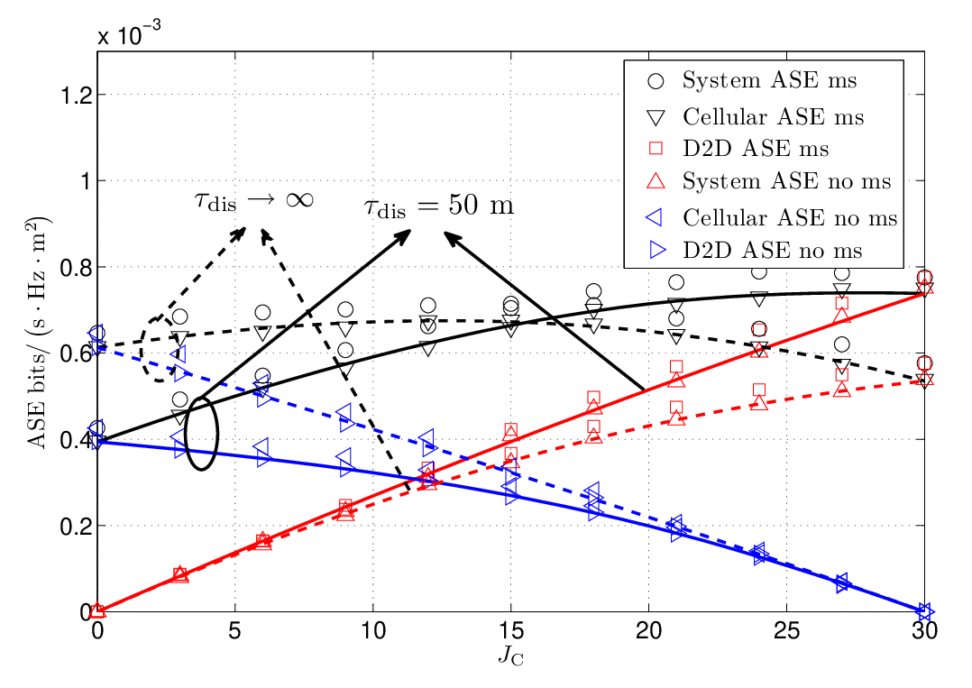
Figure 7: Codebook allocation in D2D overlaid cellular network. System parameters are set as λBS=5×10⁻⁵​BSs/m2\lambda_{\mathrm{BS}}=5\times 10^{-5}\>\mathrm{BSs/\mathrm{m}^{2}}, λU=1×10⁻³​users/m2\lambda_{\mathrm{U}}=1\times 10^{-3}\>\mathrm{users/\mathrm{m}^{2}} and λD=2.5×10⁻³​users/m2\lambda_{\mathrm{D}}=2.5\times 10^{-3}\>\mathrm{users/\mathrm{m}^{2}}. In (b), we set τdis→∞\tau_{\mathrm{dis}}\rightarrow\infty such that all D2D users select D2D mode for data transmission.

We finally investigate the performance of the D2D overlaid cellular network when different codebook allocation schemes are applied in Fig. 7. Fig. 7a shows the cellular network ASE, D2D network ASE and system ASE as a function of the number of codebooks allocated to cellular network. It is shown that allocating more codebooks to cellular (D2D) network would enhance the ASE of the corresponding network. This is due to the resource allocation rule introduced in Section II-C. In particular, each cellular (D2D) user is randomly assigned with one of the available codebooks. If more codebooks are allocated, one codebook will be reused by less users, thereby resulting in less interference over one codebook. Meanwhile, Fig. 7b shows the utility function defined in (26) as a function of the number of codebooks allocated to cellular users JC∗J_{\mathrm{C}}^{*}. It is shown from the comparison between numerical results and simulation results that JC∗J_{\mathrm{C}}^{*} obtained in Theorem 3 is of high accuracy.

VI Conclusion

In this paper, we have presented a stochastic geometry based framework to investigate the performance of SCMA in D2D and cellular hybrid network, considering underlaid mode and overlaid mode. In the underlaid mode, we analytically compared SCMA with OFDMA from the perspective of ASE and quantified the ASE gain of SCMA over OFDMA in closed form. Though approximations are used, it has been shown that high accuracy can be provided. More importantly, we concluded via the comparison results that SCMA is capable of supporting massive D2D connections, as well as significantly enhancing system ASE especially in the heavily loaded network. Therefore, SCMA can be considered as a candidate of effective multiple access schemes in future 5G wireless networks. In addition, spectrum sharing in the two coexisting modes has been studied. Specifically, the optimal D2D activated probability has been derived in the underlaid mode and the optimal codebook allocation rule has been obtained in the overlaid mode. In both cases, the optimization targets are to maximize the proportional fairness utility function. The results can serve as a guide to help tune system design parameters in SCMA enhanced D2D and cellular hybrid network.
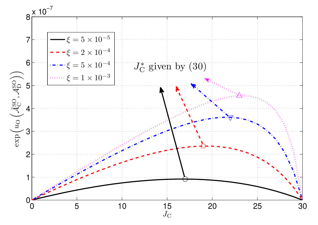
Appendix A *

A-A Proof for Proposition 1

According to (10), we have

CPBSOU\displaystyle\mathrm{CP}_{\mathrm{BS}}^{\mathrm{OU}} =ℙ{PU​rU,0−α​‖hBS0,U0‖2IC,CO+IC,DO>τBS}=ℙ{‖hBS0,U0‖2>τBS​rU,0αPU(IC,CO+IC,DO)}\displaystyle=\mathbb{P}\left\{\frac{P_{\mathrm{U}}r_{\mathrm{U},0}^{-\alpha}\left\|h_{\mathrm{BS}_{0},\mathrm{U}_{0}}\right\|^{2}}{I_{\mathrm{C},\mathrm{C}}^{\mathrm{O}}+I_{\mathrm{C},\mathrm{D}}^{\mathrm{O}}}>\tau_{\mathrm{BS}}\right\}=\mathbb{P}\left\{\left\|h_{\mathrm{BS}_{0},\mathrm{U}_{0}}\right\|^{2}>\frac{\tau_{\mathrm{BS}}r_{\mathrm{U},0}^{\alpha}}{P_{\mathrm{U}}}\left(I_{\mathrm{C},\mathrm{C}}^{\mathrm{O}}+I_{\mathrm{C},\mathrm{D}}^{\mathrm{O}}\right)\right\}
=(a)​ℒIC,CO​(sBSO)​ℒIC,DO​(sBSO),\displaystyle\overset{\left(\mathrm{a}\right)}{=}\mathcal{L}_{I_{\mathrm{C},\mathrm{C}}^{\mathrm{O}}}\left(s_{\mathrm{BS}}^{\mathrm{O}}\right)\mathcal{L}_{I_{\mathrm{C},\mathrm{D}}^{\mathrm{O}}}\left(s_{\mathrm{BS}}^{\mathrm{O}}\right), (34)

where (a) follows due to ‖hBS0,U0‖2∼exp⁡(1)\left\|h_{\mathrm{BS}_{0},\mathrm{U}_{0}}\right\|^{2}\sim\exp\left(1\right). ℒIC,CO​(sBSO)\mathcal{L}_{I_{\mathrm{C},\mathrm{C}}^{\mathrm{O}}}\left(s_{\mathrm{BS}}^{\mathrm{O}}\right) and ℒIC,DO​(sBSO)\mathcal{L}_{I_{\mathrm{C},\mathrm{D}}^{\mathrm{O}}}\left(s_{\mathrm{BS}}^{\mathrm{O}}\right), respectively, denote the Laplace transforms of IC,COI_{\mathrm{C},\mathrm{C}}^{\mathrm{O}} and IC,DOI_{\mathrm{C},\mathrm{D}}^{\mathrm{O}} evaluated at sBSO=τBS​rU,0αPUs_{\mathrm{BS}}^{\mathrm{O}}=\frac{\tau_{\mathrm{BS}}r_{\mathrm{U},0}^{\alpha}}{P_{\mathrm{U}}}. We evaluate ℒIC,CO​(sBSO)\mathcal{L}_{I_{\mathrm{C},\mathrm{C}}^{\mathrm{O}}}\left(s_{\mathrm{BS}}^{\mathrm{O}}\right) as

ℒIC,CO​(sBSO)\displaystyle\mathcal{L}_{I_{\mathrm{C},\mathrm{C}}^{\mathrm{O}}}\left(s_{\mathrm{BS}}^{\mathrm{O}}\right) =(a)​𝔼​[∏Ui∈Π~UTO​11+sBSO​PU​‖Ui−BS0‖−α]\displaystyle\overset{\left(\mathrm{a}\right)}{=}\mathbb{E}\left[\underset{\tiny{\mathrm{U}_{i}\in\tilde{\Pi}_{\mathrm{UT}}^{\mathrm{O}}}}{\prod}\frac{1}{1+s_{\mathrm{BS}}^{\mathrm{O}}P_{\mathrm{U}}\left\|\mathrm{U}_{i}-\mathrm{BS}_{0}\right\|^{-\alpha}}\right]
=(b)exp[−2πqUO​λUTK∫rU,0∞l(1−11+sBSO​PU​l−α)dl]\displaystyle\overset{\left(\mathrm{b}\right)}{=}\exp\left[-2\pi\frac{q_{\mathrm{U}}^{\mathrm{O}}\lambda_{\mathrm{UT}}}{K}\int_{r_{\mathrm{U},0}}^{\infty}l\left(1-\frac{1}{1+s_{\mathrm{BS}}^{\mathrm{O}}P_{\mathrm{U}}l^{-\alpha}}\right)dl\right]
=exp⁡[−2​π​qUO​λUT​sBSO​PUK⁡(α−2)​rU,0α−2​F12​(1,1−δ,2−δ,−rU,0−α​sBSO​PU)],\displaystyle=\exp\left[-\frac{2\pi q_{\mathrm{U}}^{\mathrm{O}}\lambda_{\mathrm{UT}}s_{\mathrm{BS}}^{\mathrm{O}}P_{\mathrm{U}}}{K\left(\alpha-2\right)r_{\mathrm{U},0}^{\alpha-2}}{}_{2}F_{1}\left(1,1-\delta,2-\delta,-r_{\mathrm{U},0}^{-\alpha}s_{\mathrm{BS}}^{\mathrm{O}}P_{\mathrm{U}}\right)\right], (35)

where (a) follows due to ‖hBS0,Ui‖2∼exp⁡(1)\left\|h_{\mathrm{BS}_{0},\mathrm{U}_{i}}\right\|^{2}\sim\exp\left(1\right) and (b) follows due to the probability generating functional (PGFL) of PPP and cellular association rule that U0\mathrm{U}_{0} connects to the nearest BS so that interfering cellular users are at least r0r_{0} away. Therefore, ℒIC,CO​(τBS​rU,0αPU)\mathcal{L}_{I_{\mathrm{C},\mathrm{C}}^{\mathrm{O}}}\left(\frac{\tau_{\mathrm{BS}}r_{\mathrm{U},0}^{\alpha}}{P_{\mathrm{U}}}\right) can be obtained by substituting sBSO=τBS​rU,0αPUs_{\mathrm{BS}}^{\mathrm{O}}=\frac{\tau_{\mathrm{BS}}r_{\mathrm{U},0}^{\alpha}}{P_{\mathrm{U}}} into (35). Following similar approach, it is easy to derive ℒIC,DO​(τBS​rU,0αPU)=exp⁡[−2​π2​λDT​(τBS​PDPU)δ​rU,02K​α​sin⁡(2​πα)]\mathcal{L}_{I_{\mathrm{C},\mathrm{D}}^{\mathrm{O}}}\left(\frac{\tau_{\mathrm{BS}}r_{\mathrm{U},0}^{\alpha}}{P_{\mathrm{U}}}\right)=\exp\left[-\frac{2\pi^{2}\lambda_{\mathrm{DT}}\left(\frac{\tau_{\mathrm{BS}}P_{\mathrm{D}}}{P_{\mathrm{U}}}\right)^{\delta}r_{\mathrm{U},0}^{2}}{K\alpha\sin\left(\frac{2\pi}{\alpha}\right)}\right].

Due to the association rule of cellular users, the CDF of rU,0r_{\mathrm{U},0} can be obtained according to the contact distribution [19], i.e., FrU,0​(x)=1−exp⁡(−π​λBS​x2)F_{r_{\mathrm{U},0}}\left(x\right)=1-\exp\left(-\pi\lambda_{\mathrm{BS}}x^{2}\right) (x≥0)\left(x\geq 0\right). Thus, the PDF of rU,0r_{\mathrm{U},0} can be accordingly obtained as frU,0​(x)=2​π​λBS​x​exp⁡(−π​λBS​x2)f_{r_{\mathrm{U},0}}\left(x\right)=2\pi\lambda_{\mathrm{BS}}x\exp\left(-\pi\lambda_{\mathrm{BS}}x^{2}\right) (x≥0)\left(x\geq 0\right). Combining ℒIC,CO​(τBS​rU,0αPU)\mathcal{L}_{I_{\mathrm{C},\mathrm{C}}^{\mathrm{O}}}\left(\frac{\tau_{\mathrm{BS}}r_{\mathrm{U},0}^{\alpha}}{P_{\mathrm{U}}}\right) and ℒIC,DO​(τBS​rU,0αPU)\mathcal{L}_{I_{\mathrm{C},\mathrm{D}}^{\mathrm{O}}}\left(\frac{\tau_{\mathrm{BS}}r_{\mathrm{U},0}^{\alpha}}{P_{\mathrm{U}}}\right) and taking the expectation of rU,0r_{\mathrm{U},0}, we derive the coverage probability at the typical cellular BS. Using similar approach, we have

CPDROU=exp⁡[−2​π2​τDRδ​rD,02K​α​sin⁡(2​πα)​(λDT+qUO​λUT​(PUPD)δ)].\mathrm{CP}_{\mathrm{DR}}^{\mathrm{OU}}=\exp\left[-\frac{2\pi^{2}\tau_{\mathrm{DR}}^{\delta}r_{\mathrm{D},0}^{2}}{K\alpha\sin\left(\frac{2\pi}{\alpha}\right)}\left(\lambda_{\mathrm{DT}}+q_{\mathrm{U}}^{\mathrm{O}}\lambda_{\mathrm{UT}}\left(\frac{P_{\mathrm{U}}}{P_{\mathrm{D}}}\right)^{\delta}\right)\right]. (36)

By taking the expectation of rD,0r_{\mathrm{D},0} in (36) according to the PDF given in (1), we derive the coverage probability at the typical D2D receiver. Note that rD,0∈[0,τdis]r_{\mathrm{D},0}\in\left[0,\tau_{\mathrm{dis}}\right], since mode selection is applied by D2D transmitters.

A-B Proof for Proposition 2

We denote ∑m=1NC​‖hBS0,U0,m‖2\underset{m=1}{\overset{N_{\mathrm{C}}}{\sum}}\left\|h_{\mathrm{BS}_{0},\mathrm{U}_{0},m}\right\|^{2} by GBS0,U0G_{\mathrm{BS}_{0},\mathrm{U}_{0}}. Since ‖hBS0,U0,m‖2∼exp⁡(1)\left\|h_{\mathrm{BS}_{0},\mathrm{U}_{0},m}\right\|^{2}\sim\exp\left(1\right), GBS0,U0G_{\mathrm{BS}_{0},\mathrm{U}_{0}} follows Gamma distribution, i.e., GBS0,U0∼Gamma⁡(NC,1)G_{\mathrm{BS}_{0},\mathrm{U}_{0}}\sim\mathrm{Gamma}\left(N_{\mathrm{C}},1\right), which makes it difficult to derive the explicit-form result of CPBSSU\mathrm{CP}_{\mathrm{BS}}^{\mathrm{SU}}. In order to provide analytical tractability, we use a random variable WBS0,U0W_{\mathrm{BS}_{0},\mathrm{U}_{0}} with mean NCN_{\mathrm{C}}, i.e., WBS0,U0∼exp⁡(NC−1)W_{\mathrm{BS}_{0},\mathrm{U}_{0}}\sim\exp\left(N_{\mathrm{C}}^{-1}\right) to approximate GBS0,U0G_{\mathrm{BS}_{0},\mathrm{U}_{0}}. Note that GBS0,U0G_{\mathrm{BS}_{0},\mathrm{U}_{0}} and WBS0,U0W_{\mathrm{BS}_{0},\mathrm{U}_{0}} have the same first moment. Therefore, we have the approximation

CPBSSU\displaystyle\mathrm{CP}_{\mathrm{BS}}^{\mathrm{SU}} ≈ℙ{PU†​rU,0−α​WBS0,U0IC,CS+IC,DS>τBS}=ℒIC,CS(sBSS)ℒIC,DS(sBSS),\displaystyle\approx\mathbb{P}\left\{\frac{P_{\mathrm{U}}^{\dagger}r_{\mathrm{U},0}^{-\alpha}W_{\mathrm{BS}_{0},\mathrm{U}_{0}}}{I_{\mathrm{C},\mathrm{C}}^{\mathrm{S}}+I_{\mathrm{C},\mathrm{D}}^{\mathrm{S}}}>\tau_{\mathrm{BS}}\right\}=\mathcal{L}_{I_{\mathrm{C},\mathrm{C}}^{\mathrm{S}}}\left(s_{\mathrm{BS}}^{\mathrm{S}}\right)\mathcal{L}_{I_{\mathrm{C},\mathrm{D}}^{\mathrm{S}}}\left(s_{\mathrm{BS}}^{\mathrm{S}}\right), (37)

where ℒIC,CS​(sBSS)\mathcal{L}_{I_{\mathrm{C},\mathrm{C}}^{\mathrm{S}}}\left(s_{\mathrm{BS}}^{\mathrm{S}}\right) and ℒIC,DS​(sBSS)\mathcal{L}_{I_{\mathrm{C},\mathrm{D}}^{\mathrm{S}}}\left(s_{\mathrm{BS}}^{\mathrm{S}}\right), respectively, denote the Laplace transforms of IC,CSI_{\mathrm{C},\mathrm{C}}^{\mathrm{S}} and IC,DSI_{\mathrm{C},\mathrm{D}}^{\mathrm{S}} evaluated at sBSS=τBS​rU,0αNC​PU†s_{\mathrm{BS}}^{\mathrm{S}}=\frac{\tau_{\mathrm{BS}}r_{\mathrm{U},0}^{\alpha}}{N_{\mathrm{C}}P_{\mathrm{U}}^{\dagger}}. We denote ∑m=1NC​‖hBS0,Ui,m‖2\overset{N_{\mathrm{C}}}{\underset{m=1}{\sum}}\left\|h_{\mathrm{BS}_{0},\mathrm{U}_{i},m}\right\|^{2} as GBS0,UiG_{\mathrm{BS}_{0},\mathrm{U}_{i}} and calculate ℒIC,CS​(sBSS)\mathcal{L}_{I_{\mathrm{C},\mathrm{C}}^{\mathrm{S}}}\left(s_{\mathrm{BS}}^{\mathrm{S}}\right) as

ℒIC,CS​(sBSS)\displaystyle\mathcal{L}_{I_{\mathrm{C},\mathrm{C}}^{\mathrm{S}}}\left(s_{\mathrm{BS}}^{\mathrm{S}}\right) =𝔼⁡[exp⁡(−∑Ui∈Π~UTS​sBSS​PU†​GBS0,Ui​‖Ui−BS0‖−α)]\displaystyle=\mathbb{E}\left[\exp\left(-\underset{\tiny{\mathrm{U}_{i}\in\tilde{\Pi}_{\mathrm{UT}}^{\mathrm{S}}}}{\sum}s_{\mathrm{BS}}^{\mathrm{S}}P_{\mathrm{U}}^{\dagger}G_{\mathrm{BS}_{0},\mathrm{U}_{i}}\left\|\mathrm{U}_{i}-\mathrm{BS}_{0}\right\|^{-\alpha}\right)\right]
=(a)​𝔼​[∏Ui∈Π~UTS​1(1+sBSS​PU†​‖Ui−BS0‖−α)NC]\displaystyle\overset{\left(\mathrm{a}\right)}{=}\mathbb{E}\left[\underset{\tiny{\mathrm{U}_{i}\in\tilde{\Pi}_{\mathrm{UT}}^{\mathrm{S}}}}{\prod}\frac{1}{\left(1+s_{\mathrm{BS}}^{\mathrm{S}}P_{\mathrm{U}}^{\dagger}\left\|\mathrm{U}_{i}-\mathrm{BS}_{0}\right\|^{-\alpha}\right)^{N_{\mathrm{C}}}}\right]
=exp[−2πqUS​λUTJ∫rU,0∞l(1−1(1+sBSS​PU†​l−α)NC)dl]\displaystyle=\exp\left[-2\pi\frac{q_{\mathrm{U}}^{\mathrm{S}}\lambda_{\mathrm{UT}}}{J}\int_{r_{\mathrm{U},0}}^{\infty}l\left(1-\frac{1}{\left(1+s_{\mathrm{BS}}^{\mathrm{S}}P_{\mathrm{U}}^{\dagger}l^{-\alpha}\right)^{N_{\mathrm{C}}}}\right)dl\right]
=exp⁡[−π​qUS​λUTrU,0−2​J​(F12​(NC,−δ,1−δ,−rU,0−α​sBSS​PU†)−1)],\displaystyle=\exp\left[-\frac{\pi q_{\mathrm{U}}^{\mathrm{S}}\lambda_{\mathrm{UT}}}{r_{\mathrm{U},0}^{-2}J}\left({}_{2}F_{1}\left(N_{\mathrm{C}},-\delta,1-\delta,-r_{\mathrm{U},0}^{-\alpha}s_{\mathrm{BS}}^{\mathrm{S}}P_{\mathrm{U}}^{\dagger}\right)-1\right)\right], (38)

where (a) is due to the PGFL of PPP. Likewise, we calculate ℒIC,DS​(sBSS)\mathcal{L}_{I_{\mathrm{C},\mathrm{D}}^{\mathrm{S}}}\left(s_{\mathrm{BS}}^{\mathrm{S}}\right) as

ℒIC,DS​(sBSS)\displaystyle\mathcal{L}_{I_{\mathrm{C},\mathrm{D}}^{\mathrm{S}}}\left(s_{\mathrm{BS}}^{\mathrm{S}}\right) =𝔼⁡[exp⁡(−∑DTj∈ΠDTS​sBSS​PD†​GBS0,DTi​‖DTj−BS0‖−α)]\displaystyle=\mathbb{E}\left[\exp\left(-\underset{\tiny{\mathrm{DT}_{j}\in\Pi_{\mathrm{DT}}^{\mathrm{S}}}}{\sum}s_{\mathrm{BS}}^{\mathrm{S}}P_{\mathrm{D}}^{\dagger}G_{\mathrm{BS}_{0},\mathrm{DT}_{i}}\left\|\mathrm{DT}_{j}-\mathrm{BS}_{0}\right\|^{-\alpha}\right)\right]
=𝔼⁡[∏DTj∈ΠDTS​1(1+sBSS​PD†​‖DTi−BS0‖−α)NC]\displaystyle=\mathbb{E}\left[\underset{\tiny{\mathrm{DT}_{j}\in\Pi_{\mathrm{DT}}^{\mathrm{S}}}}{\prod}\frac{1}{\left(1+s_{\mathrm{BS}}^{\mathrm{S}}P_{\mathrm{D}}^{\dagger}\left\|\mathrm{DT}_{i}-\mathrm{BS}_{0}\right\|^{-\alpha}\right)^{N_{\mathrm{C}}}}\right]
=(a)exp[−2πλDTJ∫0∞l(1−1(1+sBSS​PD†​l−α)NC)dl]\displaystyle\overset{\left(\mathrm{a}\right)}{=}\exp\left[-2\pi\frac{\lambda_{\mathrm{DT}}}{J}\int_{0}^{\infty}l\left(1-\frac{1}{\left(1+s_{\mathrm{BS}}^{\mathrm{S}}P_{\mathrm{D}}^{\dagger}l^{-\alpha}\right)^{N_{\mathrm{C}}}}\right)dl\right]
=exp⁡[−2​π2​λDT​(sBSS​PD†)δJ​α​sin⁡(2​πα)​∏n=2⁡NC⁡​(2(n−1)​α+1)],\displaystyle=\exp\left[-\frac{2\pi^{2}\lambda_{\mathrm{DT}}\left(s_{\mathrm{BS}}^{\mathrm{S}}P_{\mathrm{D}}^{\dagger}\right)^{\delta}}{J\alpha\sin\left(\frac{2\pi}{\alpha}\right)}\underset{{}_{n=2}}{\overset{{}_{N_{\mathrm{C}}}}{\prod}}\left(\frac{2}{\left(n-1\right)\alpha}+1\right)\right], (39)

where (a) follows because all D2D transmitters are active.

Substituting sBSS=τBS​rU,0αNC​PU†s_{\mathrm{BS}}^{\mathrm{S}}=\frac{\tau_{\mathrm{BS}}r_{\mathrm{U},0}^{\alpha}}{N_{\mathrm{C}}P_{\mathrm{U}}^{\dagger}} into (38) and (39), we have

ℒIC,CS​(τBS​rU,0αNC​PU†)=exp⁡[−π​qUS​λUTJ​rU,02​(F12​(NC,−δ,1−δ,−τBSNC)−1)].\mathcal{L}_{I_{\mathrm{C},\mathrm{C}}^{\mathrm{S}}}\left(\frac{\tau_{\mathrm{BS}}r_{\mathrm{U},0}^{\alpha}}{N_{\mathrm{C}}P_{\mathrm{U}}^{\dagger}}\right)=\exp\left[-\pi\frac{q_{\mathrm{U}}^{\mathrm{S}}\lambda_{\mathrm{UT}}}{J}r_{\mathrm{U},0}^{2}\left({}_{2}F_{1}\left(N_{\mathrm{C}},-\delta,1-\delta,-\frac{\tau_{\mathrm{BS}}}{N_{\mathrm{C}}}\right)-1\right)\right]. (40)
ℒIC,DS​(τBS​rU,0αNC​PU†)=exp⁡[−2​π2​λDT​(τBS​PD†NC​PU†)δ​rU,02J​α​sin⁡(2​πα)​∏n=2⁡NC⁡​(2(n−1)​α+1)].\mathcal{L}_{I_{\mathrm{C},\mathrm{D}}^{\mathrm{S}}}\left(\frac{\tau_{\mathrm{BS}}r_{\mathrm{U},0}^{\alpha}}{N_{\mathrm{C}}P_{\mathrm{U}}^{\dagger}}\right)=\exp\left[-\frac{2\pi^{2}\lambda_{\mathrm{DT}}\left(\frac{\tau_{\mathrm{BS}}P_{\mathrm{D}}^{\dagger}}{N_{\mathrm{C}}P_{\mathrm{U}}^{\dagger}}\right)^{\delta}r_{\mathrm{U},0}^{2}}{J\alpha\sin\left(\frac{2\pi}{\alpha}\right)}\underset{{}_{n=2}}{\overset{{}_{N_{\mathrm{C}}}}{\prod}}\left(\frac{2}{\left(n-1\right)\alpha}+1\right)\right]. (41)

The PDF of rU,0r_{\mathrm{U},0} can be obtained in Appendix A-A. Therefore, we derive the approximate coverage probability at the typical BS by combining the results of (40) and (41) into (37) and taking the expectation of rU,0r_{\mathrm{U},0}.

Using similar approach, we approximate the coverage probability at the typical D2D receiver and then complete the proof. The detail of derivation steps is omitted due to space limitation.

References

  • [1] Cisco, “Global mobile data traffic forecast update,” white paper, Feb. 2011.
  • [2] Ericsson, “More than 50 billion connected devices,” white paper, Feb. 2011.
  • [3] D. Feng, L. Lu, Y. Yuan-Wu, G. Li, S. Li, and G. Feng, “Device-to-device communications in cellular networks,” IEEE Commun. Mag., vol. 52, no. 4, pp. 49–55, Apr. 2014.
  • [4] A. Asadi, Q. Wang, and V. Mancuso, “A survey on device-to-device communication in cellular networks,” IEEE Commun. Surveys Tuts., vol. 16, no. 4, pp. 1801–1819, Fourthquarter 2014.
  • [5] L. Lei, Z. Zhong, C. Lin, and X. Shen, “Operator controlled device-to-device communications in LTE-advanced networks,” IEEE Wireless Commun., vol. 19, no. 3, pp. 96–104, Jun. 2012.
  • [6] X. Lin, J. Andrews, and A. Ghosh, “Spectrum sharing for device-to-device communication in cellular networks,” IEEE Trans. Wireless Commun., vol. 13, no. 12, pp. 6727–6740, Dec. 2014.
  • [7] M. Sheng, J. Liu, Y. Zhang, H. Sun, and J. Li, “On transmission capacity region of D2D integrated cellular networks with interference management,” IEEE Trans. Commun., vol. 63, no. 4, pp. 1383–1399, Apr. 2015.
  • [8] N. Lee, X. Lin, J. Andrews, and R. Heath, “Power control for D2D underlaid cellular networks: Modeling, algorithms, and analysis,” IEEE J. Sel. Areas Commun., vol. 33, no. 1, pp. 1–13, Jan. 2015.
  • [9] C.-H. Yu, K. Doppler, C. Ribeiro, and O. Tirkkonen, “Resource sharing optimization for device-to-device communication underlaying cellular networks,” IEEE Trans. Wireless Commun., vol. 10, no. 8, pp. 2752–2763, Aug. 2011.
  • [10] Y. Pei and Y. chang Liang, “Resource allocation for device-to-device communications overlaying two-way cellular networks,” IEEE Trans. Wireless Commun., vol. 12, no. 7, pp. 3611–3621, Jul. 2013.
  • [11] S. Zhang, J. Liu, N. Kato, H. Ujikawa, and K. Suzuki, “Average rate analysis for a D2D overlaying two-tier downlink cellular network,” in Proc. IEEE ICC, London, UK, Jun. 2015, pp. 3376–3381.
  • [12] C. Y. Wong, R. Cheng, K. Lataief, and R. Murch, “Multiuser OFDM with adaptive subcarrier, bit, and power allocation,” IEEE J. Sel. Areas Commun., vol. 17, no. 10, pp. 1747–1758, Oct. 1999.
  • [13] H. Nikopour and H. Baligh, “Sparse code multiple access,” in Proc. IEEE PIMRC, London, UK, Sep. 2013, pp. 332–336.
  • [14] M. Taherzadeh, H. Nikopour, A. Bayesteh, and H. Baligh, “SCMA codebook design,” in Proc. IEEE VTC Fall, Vancouver, Canada, Sep. 2014, pp. 1–5.
  • [15] M. Ni, L. Zheng, F. Tong, J. Pan, and L. Cai, “A geometrical-based throughput bound analysis for device-to-device communications in cellular networks,” IEEE J. Sel. Areas Commun., vol. 33, no. 1, pp. 100–110, Jan. 2015.
  • [16] K. Zhu and E. Hossain, “Joint mode selection and spectrum partitioning for device-to-device communication: A dynamic stackelberg game,” IEEE Trans. Wireless Commun., vol. 14, no. 3, pp. 1406–1420, Mar. 2015.
  • [17] F. Baccelli, J. Li, T. Richardson, S. Shakkottai, S. Subramanian, and X. Wu, “On optimizing CSMA for wide area ad hoc networks,” Queueing Syst., vol. 72, no. 1-2, pp. 31–68, Oct. 2012. [Online]. Available: http://dx.doi.org/10.1007/s11134-012-9289-7
  • [18] H. ElSawy, E. Hossain, and M.-S. Alouini, “Analytical modeling of mode selection and power control for underlay D2D communication in cellular networks,” IEEE Trans. Commun., vol. 62, no. 11, pp. 4147–4161, Nov. 2014.
  • [19] D. Stoyan, W. S. Kendall, J. Mecke, and L. Ruschendorf, Stochastic geometry and its applications. Wiley Chichester, 1995, vol. 2.
  • [20] R. Hoshyar, F. Wathan, and R. Tafazolli, “Novel low-density signature for synchronous CDMA systems over AWGN channel,” IEEE Trans. Signal Process., vol. 56, no. 4, pp. 1616–1626, Apr. 2008.
  • [21] M.-S. Alouini and A. Goldsmith, “Area spectral efficiency of cellular mobile radio systems,” IEEE Trans. Veh. Technol., vol. 48, no. 4, pp. 1047–1066, Jul. 1999.
  • [22] A. Sakr and E. Hossain, “Cognitive and energy harvesting-based D2D communication in cellular networks: Stochastic geometry modeling and analysis,” IEEE Trans. Commun., vol. 63, no. 5, pp. 1867–1880, May 2015.
  • [23] H. ElSawy and E. Hossain, “Two-tier HetNets with cognitive femtocells: Downlink performance modeling and analysis in a multichannel environment,” IEEE Trans. Mobile Comput., vol. 13, no. 3, pp. 649–663, Mar. 2014.
  • [24] B. Stephen and V. Lieven, Convex optimization. Cambridge Univ. Press, 2004.
  • [25] K. Huang, V. Lau, and Y. Chen, “Spectrum sharing between cellular and mobile ad hoc networks: transmission-capacity trade-off,” IEEE J. Sel. Areas Commun., vol. 27, no. 7, pp. 1256–1267, Sep. 2009.