Radiative and mechanical feedback into the molecular gas in the Large Magellanic Cloud. I. N159WThanks: Herschel is an ESA space observatory with science instruments provided by European-led Principal Investigator consortia and with important participation from NASA.
Abstract
We present Herschel SPIRE Fourier Transform Spectrometer (FTS) observations of N159W, an active star-forming region in the Large Magellanic Cloud (LMC). In our observations, a number of far-infrared cooling lines including CO to , CI 609 m and 370 m, and NII 205 m are clearly detected. With an aim of investigating the physical conditions and excitation processes of molecular gas, we first construct CO spectral line energy distributions (SLEDs) on 10 pc scales by combining the FTS CO transitions with ground-based low- CO data and analyze the observed CO SLEDs using non-LTE radiative transfer models. We find that the CO-traced molecular gas in N159W is warm (kinetic temperature of 153–754 K) and moderately dense (H2 number density of (1.1–4.5) 103 cm-3). To assess the impact of the energetic processes in the interstellar medium on the physical conditions of the CO-emitting gas, we then compare the observed CO line intensities with the models of photodissociation regions (PDRs) and shocks. We first constrain the properties of PDRs by modelling Herschel observations of OI 145 m, CII 158 m, and CI 370 m fine-structure lines and find that the constrained PDR components emit very weak CO emission. X-rays and cosmic-rays are also found to provide a negligible contribution to the CO emission, essentially ruling out ionizing sources (ultraviolet photons, X-rays, and cosmic-rays) as the dominant heating source for CO in N159W. On the other hand, mechanical heating by low-velocity C-type shocks with 10 km s-1 appears sufficient enough to reproduce the observed warm CO.
Key Words.
ISM: molecules – galaxies: individual: Magellanic Clouds – galaxies: ISM – Infrared: ISM1 Introduction
Star formation exclusively occurs in molecular clouds, the densest component of the interstellar medium (ISM) (e.g., Kennicutt & Evans 2012). The main constituent of these molecular clouds is molecular hydrogen (H2), which is, unfortunately, not directly observable in the typical conditions of cold molecular gas due to its symmetric, homonuclear nature. The strong rotational transitions of carbon monoxide (12CO; simply CO hereafter) at mm and sub-mm wavelengths have instead been used as common tracers of molecular gas. In particular, CO rotational lines have a wide range of critical densities, making them accessible probes of the physical conditions of molecular gas in diverse environments (e.g., kinetic temperature 10–1000 K and hydrogen density 103–108 cm-3).
The diagnostic power of CO rotational transitions has been considerably further exploited since the advent of the ESA Herschel Space Observatory (Pilbratt et al. 2010). In combination with ground-based telescope data, Photodector Array Camera and Spectrometer (PACS; Poglitsch et al. 2010), Spectral and Photometric Imaging Receiver (SPIRE; Griffin et al. 2010), and Heterodyne Instrument for the Far Infrared (HIFI; de Graauw et al. 2010) spectroscopic observations have enabled us to construct CO spectral line energy distributions (SLEDs) from the upper level = 1 to 50. In the past several years, Herschel-based CO SLEDs have been extensively examined for a wide range of Galactic (e.g., photodissociation regions (PDRs): Habart et al. 2010; Köhler et al. 2014; Pon et al. 2014; Stock et al. 2015; protostars: Larson et al. 2015) and extragalactic sources (e.g., infrared (IR)-bright galaxies: Rangwala et al. 2011; Kamenetzky et al. 2012; Meijerink et al. 2013; Pellegrini et al. 2013; Greve et al. 2014; Lu et al. 2014; Papadopoulos et al. 2014; Rosenberg et al. 2014; Schirm et al. 2014; Mashian et al. 2015; Wu et al. 2015b; Seyfert galaxies: van der Werf et al. 2010; Hailey-Dunsheath et al. 2012; Israel et al. 2014), revealing the ubiquitous presence of warm molecular gas ( 100 K). Various heating sources, e.g., ultraviolet (UV) photons, X-rays, and cosmic-rays, have been invoked to explain the properties of this warm molecular gas and the emerging picture is that non-ionizing sources such as mechanical heating (e.g., shocks driven by merging activities, stellar winds, and supernova explosions) must play a critical role.


In this paper, we aim at probing the physical conditions and excitation processes of molecular gas traced by CO emission in detail on individual molecular cloud scales. To do so, we study N159W, an active star-forming region in the Large Magellanic Cloud (LMC), largely based on Herschel PACS and SPIRE observations. The LMC is an excellent laboratory for our study for the following reasons. First of all, the proximity of the LMC (distance of 50 kpc; e.g., Pietrzyński et al. 2013) enables us to perform high-resolution observations of spatially-resolved molecular clouds. In addition, the LMC is located at high Galactic latitude and has an almost face-on orientation (inclination angle of 35∘; e.g., van der Marel & Cioni 2001), providing a view with less confusion and low interstellar extinction.
N159W is one of the three prominent molecular clouds in the HII region complex N159 (Figure 1) and its stellar and gas contents have been extensively studied at multiple wavelengths. For example, previous optical and near IR studies have identified a large number of O- and B-type stars, embedded young stellar objects (YSOs), and ultracompact HII regions (e.g., Jones et al. 2005; Fariña et al. 2009; Chen et al. 2010; Carlson et al. 2012), suggesting that N159W is one of the most intense star-forming regions in the LMC. As the brightest CO(1–0) peak in the LMC (e.g., Johansson et al. 1994; Fukui et al. 1999; Wong et al. 2011), N159W has been frequently targeted for radio, mm, and sub-mm observations as well. The Australia Telescope Compact Array (ATCA) and the Atacama Large Millimeter/submillimeter Array (ALMA) have provided the sharpest view of molecular gas so far (Seale et al. 2012; Fukui et al. 2015), revealing the complex filamentary distributions of CO(2–1), 13CO(2–1), HCO+(1–0), and HCN(1–0). The presence of high excitation molecular gas was hinted by CO(4–3), CO(6–5), and CO(7–6) observations by Bolatto et al. (2005), Pineda et al. (2008), Mizuno et al. (2010), and Okada et al. (2015).
Besides the extensive observations at multiple wavelengths, the presence of various energetic sources makes N159W an ideal target for our study. As described in the previous paragraph, numerous OB-type stars and YSOs exist in the region and they can produce UV photons and strong stellar outflows. In addition, the nearby black hole binary LMC X-1, the most luminous X-ray source in the LMC (X-ray luminosity of 1038 erg s-1; Schlegel et al. 1994), can have a substantial influence on the surrounding ISM. Compared to UV photons, X-rays penetrate deeper into molecular clouds while dissociating fewer molecules. As a result, X-rays produce larger column densities of warm molecular gas for a given irradiation energy (e.g., Meijerink & Spaans 2005). The supernova remnant (SNR) J0540.0–6944 and its expanding shell are located just 75 pc from N159W (e.g., Chu et al. 1997; Williams et al. 2000) and can be another source of heating. Last but not least, a number of studies have indicated that the “molecular ridge” where N159W is located may have been exposed to large-scale energetic events driven by multiple supernova explosions, tidal force, and/or ram pressure. The molecular ridge is the largest molecular concentration in the LMC, comprising 30% of the total molecular mass in the galaxy (e.g., Mizuno et al. 2001). The distribution of star formation across the ridge is quite intriguing, increasing from south to north toward the starbursting 30 Doradus region, and this has led several authors to suggest sequential star formation. For example, de Boer et al. (1998) proposed that the motion of the LMC through the hot halo gas of the Milky Way created bow shocks at the leading edge, consequently triggering the sequential star formation. This leading edge of the LMC corresponds to the southeastern HI overdensity region, which appears to merge into the Small Magellanic Cloud (SMC) through the Magellanic Bridge connecting the two Magellanic Clouds (e.g., Kim et al. 1998; Putman et al. 2003). Since the Magellanic Bridge has been considered to be formed through gravitational interactions between the two Magellanic Clouds (e.g., Bekki & Chiba 2007; Besla et al. 2012), this hints that the tidal force could be at work in the HI overdensity region. The HI overdensity region has also been shown to harbour several supergiant and giant HI shells (e.g, Kim et al. 1998; Kim et al. 1999), suggesting that powerful supernova explosions from multiple OB associations have injected a large amount of mechanical energy into the surrounding ISM. In Figure 1, we present three-color composite and HI column density images of N159W and its surrounding regions.
This paper is organized in the following way. First, we provide a description of the multiwavelength datasets used in our study (Section 2). Next, we discuss spectral line detection in our Herschel SPIRE Fourier Transform Spectrometer (FTS) observations (Section 3) and derive the physical properties of molecular gas by modelling CO lines with the non-LTE radiative transfer code RADEX (van der Tak et al. 2007) (Section 4). We then employ theoretical models of PDRs and shocks to examine the excitation conditions of CO in N159W (Section 5) and finally summarize our conclusions (Section 6).
2 Data
In this section, we describe the data in our study and summarize their main parameters (e.g., rest wavelength, FWHM, 1 uncertainty in the integrated intensity, luminosity, etc.) (Table 1).


2.1 Herschel SPIRE Spectroscopic Data
2.1.1 Observations
N159W was observed with the SPIRE FTS in the high spectral resolution ( 1.2 GHz), intermediate spatial sampling mode. The FTS has two spectrometer arrays, SPIRE Long Wavelength (SLW) and SPIRE Short Wavelength (SSW), which cover wavelength ranges of 303–671 m and 194–313 m respectively. The FTS beam profile changes with wavelength and cannot be characterized by a simple Gaussian function due to the multi-moded nature of feedhorn coupled detectors (Makiwa et al. 2013). The FTS beam size varies from 17′′ to 42′′ (corresponding to 4–10 pc at the distance of the LMC; Wu et al. 2015b) and is presented in Table 1. The SLW and SSW arrays consist of 19 and 37 detectors respectively, which are arranged in a hexagonal pattern covering a 3′ 3′ area. In the intermediate spatial sampling mode, the SLW and SSW are moved to four jiggling positions with 28′′ and 16′′ spacings respectively. The locations of all detectors are shown in Figures 1 and 3. Note that our final maps are sub-Nyquist sampled because of the detector spacing that roughly corresponds to the FTS beam size. The observations were performed on January 8, 2013 with a total integration time of 5707s (Obs. ID: 1342259066; PI: S. Hony).
2.1.2 Data Processing and Map-making
We process the FTS data using the Herschel Interactive Processing Environment (HIPE) version 11.0.2825 and the SPIRE calibration version 11.0 (Fulton et al. 2010; Swinyard et al. 2014). The calibration was obtained from measurements of Uranus and its uncertainty was estimated to be 10% (SPIRE Manual)11 1 http://herschel.esac.esa.int/Docs/SPIRE/html/spire_om.html


To derive integrated intensity images and their uncertainties, we employ the data reduction script by Wu et al. (2015b), which was recently used to successfully generate FTS cubes for M83. We first start off by performing line measurement of point source calibrated spectra for each transition. As an example, the spectra from the central SLW and SSW detectors are presented in Figure 2, with the locations of the spectral lines observed with the SPIRE FTS. In our line measurement, a combination of parabola (continuum) and sinc (emission) functions is used to fit a spectral line for the frequency range of GHz, where is the rest frequency of the line. The continuum subtracted spectra are then projected onto a common grid covering a 5′ 5′ area with a pixel size of 15′′ (roughly corresponding to the jiggle spacing of the SSW observations) to construct a spectral cube. The spectrum for each pixel is calculated as the (1/)-weighted sum of overlapping spectra, where is the 1 uncertainty provided by the pipeline. The overlapping spectra are scaled in proportion to their covering areas in the pixel before the summation. Finally, the integrated intensity (, , or ) is derived by performing line measurement of the constructed spectral cube and its uncertainty () is obtained by adding two errors in quadrature, = , where is the statistical error based on the residual from line measurement and is the calibration error of 10%.


In this paper, we combine the FTS data with other tracers of gas and dust (Sections 2.2, 2.3, and 2.4). To compare them at a common resolution, we smooth the FTS maps to 42′′ resolution (10 pc at the LMC distance), which corresponds to the FWHM for the CO(4–3) transition, by convolving with proper kernels. These kernels were generated by Wu et al. (2015b) based on the fitting of a two-dimensional Hermite-Gaussian function to the FTS beam profiles, essentially following the method by Gordon et al. (2008). In addition, we rebin the smoothed maps to have a final pixel size of 30′′, which roughly corresponds to the jiggle spacing of the SLW observations. We present the resulting integrated intensity images in Figure 3 and Appendix A and refer to Wu et al. (2015b) for details on the map-making procedure.
Finally, to cross-check our map-making procedure, we compare the FTS CO(4–3) integrated intensity image with NANTEN2 CO(4–3) observations at 38′′ resolution (Mizuno et al. 2010). For the comparison, we convolve the NANTEN2 data with a Gaussian kernel to have a final resolution of 42′′ and find that the FTS and NANTEN2 data are consistent within 1 uncertainties: the ratio of the FTS to NANTEN2 data ranges from 0.7 to 1.2, suggesting that our map-making procedure is accurate.
2.2 Herschel PACS Spectroscopic Data
N159W was observed with the PACS spectrometer on May 24, 2011, as part of the Herschel guaranteed time key project SHINING (PI: E. Sturm). The four fine-structure lines, [CII] 158 m, [OI] 63 m, [OI] 145 m, and [OIII] 88 m, were mapped in the unchoped scan mode (Obs. IDs: 1342222075 to 1342222084). As described in Poglitsch et al. (2010), the PACS spectrometer is an integral field spectrometer that consists of 25 (spatial) 16 (spectral) pixels. The spectrometer covers a wavelength range of 51–220 m with a projected footprint of 5 5 spatial pixels (“spaxels”) on the sky (corresponding to a 47′′ 47′′ field-of-view). The FWHM depends on wavelengths, ranging from 10′′ at 60 m to 12′′ at 160 m (PACS Manual)22 2 http://herschel.esac.esa.int/Docs/PACS/html/pacs_om.html.
The PACS spectroscopic data are first reduced with the HIPE version 12.0.0 (Ott 2010) from Level 0 to Level 1. The Level 1 cubes (calibrated in both flux and wavelength) are then exported and processed with PACSman (Lebouteiller et al. 2012) to create integrated intensity images. Each spectrum is fitted with a combination of polynomial (baseline) and Gaussian (line) functions and the line fluxes of all spaxels are projected onto a grid with a size of 1′ 2′. The pixel size of 3′′ (corresponding to 1/3 of the spaxel size) is chosen to recover the best spatial resolution possible. For the 1 error in the integrated intensity, the uncertainty from map projection/line measurement (; provided by PACSman) and the calibration uncertainty of 22% (; 10% for spaxel-to-spaxel variations and 12% for absolute calibration) are added in quadrature. We present final integrated intensity maps and a sample of PACS spectra in Figures 4 and 5 and refer to Lebouteiller et al. (2012) and Cormier et al. (2015) for details on the data reduction and map-making procedures.
The limited spatial coverage of the PACS data, unfortunately, results in only several pixels to work with when the maps are smoothed and regridded to match the FTS resolution (42′′) and pixel size (30′′). The common region between the PACS and FTS data at 42′′ resolution has a size of 1.0′ 1.5′ (e.g., Figure 13) and all fine-structure transitions are clearly detected with the statistical signal-to-noise ratio S/Ns (integrated intensity divided by ) > 5 (our threshold for line detection; Section 3.1).


2.3 Ground-based CO Data
2.3.1 Mopra CO(1–0) Data
We use the CO(1–0) data from the MAGellanic Mopra Assessment (MAGMA) survey (Wong et al. 2011). This survey targeted bright CO complexes that were previously identified from the NANTEN survey (Mizuno et al. 2001) and observed them with the 22 m Mopra telescope on 45′′ scales. To estimate the CO(1–0) integrated intensity, each data cube was first smoothed to 90′′ resolution and a mask was generated based on the 3 level. The generated mask was then applied to the original cube and the CO(1--0) emission within the mask was integrated from33 3 In this paper, all velocities are quoted in the Local Standard of Rest (LSR) frame. = 200 km s-1 to 305 km s-1. The uncertainty in the integrated intensity was derived by multiplying the root-mean-square (rms) noise per channel by the square root of the number of channels that contribute to the intensity map at that position. To take a systematic error into account, we combine this uncertainty with the calibration uncertainty of 25% (T. Wong, personal communication) and add them in quadrature. For the area that overlaps with the FTS coverage (2.5′ 2.5′ in size; Figure 7), the final uncertainty at 45′′ resolution has a median of 5.3 K km s-1 (Table 1) and the CO(1–0) transition is detected everywhere with S/Ns > 5.
2.3.2 ASTE CO(3–2) Data
We use the CO(3–2) data obtained by Minamidani et al. (2008). Minamidani et al. (2008) observed N159 with the 10 m Atacama Submillimeter Telescope Experiment (ASTE) telescope at 22′′ resolution. In order to derive the integrated intensity, we integrate the CO(3–2) emission from = 220 km s-1 to 250 km s-1. This velocity range is slightly different from that used to estimate the CO(1–0) integrated intensity, but the discrepancy would not make a significant impact on the CO(3–2) integrated intensity considering that the spectra contain essentially noise beyond the velocity range of 220–250 km s-1 (e.g., Figure 2 of Minamidani et al. 2008). The final uncertainty in the integrated intensity is then estimated in the same way as we do for CO(1–0): add the statistical error derived from the rms noise per channel and the calibration error of 20% (Minamidani et al. 2008) in quadrature. When smoothed to 42′′ resolution and regridded to match the FTS data, the CO(3–2) observations have a median uncertainty of 5.9 K km s-1 (Table 1) and S/Ns > 5 is achieved everywhere.
| Species | Transition | Rest Wavelengtha | FWHMc | Luminosityf,g | ||||
|---|---|---|---|---|---|---|---|---|
| (m) | (K) | (cm-3) | (′′) | (10-11 W m-2 sr-1) | (10-11 W m-2 sr-1) | (L⊙) | ||
| 12CO | =1–0 | 2600.8 | 6 | 4.7 102 | 45 | 0.1 | 0.8 | 0.90.1 |
| 12CO | =3–2 | 867.0 | 33 | 1.5 104 | 22 | 1.4 | 25.1 | 33.51.9 |
| 12CO | =4–3 | 650.3 | 55 | 3.7 104 | 42 | 15.3 | 29.4 | 67.82.2 |
| 12CO | =5–4 | 520.2 | 83 | 7.2 104 | 34 | 11.6 | 34.6 | 88.52.6 |
| 12CO | =6–5 | 433.6 | 116 | 1.3 105 | 29 | 6.6 | 36.9 | 101.53.0 |
| 12CO | =7–6 | 371.7 | 155 | 2.0 105 | 33 | 6.3 | 32.5 | 86.52.6 |
| 12CO | =8–7 | 325.2 | 199 | 2.9 105 | 33 | 17.2 | 29.4 | 71.52.6 |
| 12CO | =9–8 | 289.1 | 249 | 4.0 105 | 19 | 14.7 | 22.6 | 48.71.7 |
| 12CO | =10–9 | 260.2 | 304 | 5.3 105 | 18 | 18.3 | 22.7 | 33.41.5 |
| 12CO | =11–10 | 236.6 | 365 | 7.0 105 | 17 | 20.6 | 23.2 | 24.31.3 |
| 12CO | =12–11 | 216.9 | 431 | 9.0 105 | 17 | 17.9 | 23.2 | 18.91.1 |
| 12CO | =13–12 | 200.3 | 503 | 1.1 106 | 17 | 27.1 | 27.9 | – |
| CI | – | 609.1 | 24 | 4.9 102 | 38 | 17.9 | 20.0 | 18.81.2 |
| CI | – | 370.4 | 62 | 9.3 102 | 33 | 6.3 | 17.4 | 48.81.5 |
| CII | – | 157.7 | 91 | 2.7 103 | 12 | 368.8 | 9439.1 | 3907.2399.9 |
| OI | – | 145.5 | 327 | 1.5 105 | 12 | 88.1 | 622.7 | 250.325.4 |
| OI | – | 63.2 | 228 | 9.7 105 | 10 | 354.5 | 6444.5 | 2435.1248.9 |
| OIII | – | 88.4 | 163 | 5.0 102 | 10 | 544.8 | 1.1 104 | 5460.5600.8 |
| NII | – | 205.2 | 70 | 4.5 101 | 17 | 27.5 | 42.5 | 99.23.5 |
| – | 60–200 | – | – | 42 | – | 3.9 104 | (3.30.1) 105 | |
| – | 3–1000 | – | – | 42 | – | 8.1 104 | (7.50.1) 105 |
a Data from Leiden Atomic and Molecular Database
(except for [NII] and [OIII], whose data come from Carilli & Walter 2013).
b Critical density (CO data from Walker et al. 2015 and the rest from Tielens 2005).
For the CO, [CI], [CII], and [OI] lines, the critical densities are evaluated at the kinetic temperature of 100 K.
c Angular resolution of the original data.
d Median in the integrated intensity at 42′′ resolution ( = statistical 1 uncertainty).
e Median in the integrated intensity at 42′′ resolution
( = final 1 uncertainty; statistical and calibration errors added in quadrature).
f Luminosity derived by integrating over all pixels with S/Ns > 5 at 42′′ resolution.
g Except for CO(1–0) at 45′′ resolution.
h For CO(1–0) and CO(3–2), the conversion factors of 1.6 10-12 and 4.2 10-11
are used to convert K km s-1 into W m-2 sr-1.
d,e,f Different spatial areas are considered for the estimates:
1.0′ 1.5′ for the [CII], [OI], and [OIII] transitions
and 2.5′ 2.5′ for the rest.
2.4 Derived Dust and IR Continuum Properties
We use the dust and IR continuum properties of N159W estimated following Galametz et al. (2013). To derive these properties, Galametz et al. (2013) applied the dust spectral energy distribution (SED) model by Galliano et al. (2011) to Spitzer (3.6, 4.5, 5.8, 8, 24, and 70 m) and Herschel (100, 160, 250, 350, and 500 m) photometric data (Meixner et al. 2006, 2013). The amorphous carbon (AC) composition was used for this purpose, as it was designed to consistently reproduce the Herschel broadband emission of the LMC. It is more emissive than the standard Draine & Li (2007) model. In essence, Galliano et al. (2011)’s approach is twofold: (1) modelling of dust SED for a single mass element of the ISM with uniform illumination and (2) synthesizing several mass elements to account for the variations in illumination conditions. In the SED fitting procedure, independent free parameters are the total dust mass (), PAH-to-dust mass ratio (), index for the power-law distribution of starlight intensities (), lower cut-off for the power-law distribution of starlight intensities (), range of starlight intensities (), and mass of old stars (). Based on these free parameters, the following properties can also be estimated (Figure 6 and Table 1): far IR luminosity (60–200 m; ), total IR luminosity (3–1000 m; ), and dust temperature (). Galametz et al. (2013) derived all these parameters at 36′′ resolution and estimated their uncertainties by performing MC simulations where the measured IR fluxes were perturbed based on 1 errors and the SED fitting was repeated 20 times. In our study, we use the parameters estimated on 42′′ scales to match the FTS resolution. We refer to Galametz et al. (2013) and Galliano et al. (2011) for details on dust SED modelling.


3 Results
3.1 FTS Line Detection
We show the FTS spectra in Figure 3 and Appendix 19 and focus on CO and CI line detection in this section. A detailed analysis on the physical properties and excitation conditions of the CO-emitting gas will be presented in Sections 4 and 5. Throughout this paper, we apply a threshold of S/Ns > 5 for line detection and categorize the CO transitions into three groups (e.g., Köhler et al. 2014): low- for 5, intermediate- for 6 9, and high- for 10 where is the upper level .
In N159W, FTS CO transitions with = 4–12 are detected. These rotational lines have upper level energies of 55–431 K and critical densities of 104–106 cm-3 (Table 1; Yang et al. 2010), suggesting that they are valuable probes of molecular gas over a range of density and temperature. To estimate the total CO luminosity, we add up the integrated intensities at 42′′ resolution over all pixels with S/Ns > 5 and provide the results in Table 1. We find the total CO luminosity of = (575.56.8) L⊙ (including = 1, 3, 4, …, 12), which is 8 10-4 of the total IR luminosity. This total CO luminosity is dominated by the rotational lines with 4 8 (low- and intermediate-) and the largest contribution (20%) comes from the CO(6–5) transition. Note, however, that our estimate is limited up to = 12. Considering that the observed CO SLEDs are relatively flat up to = 12 for some pixels (Section 4.1), hinting at more CO emission at 13, the actual total CO luminosity is likely higher. To be specific, our non-LTE radiative transfer modelling (Section 4.2) suggests that high- transitions with 13 could contribute up to 8% of the total CO luminosity.44 4 This estimate is based on the assumption that there is no additional warm component emitting at 13.
Both atomic carbon fine-structure lines at 609 m and 370 m are detected in N159W. Their upper levels lie 24 K and 62 K above the ground state and their critical densities are low with 102–103 cm-3 (Table 1; Launay & Roueff 1977). Under the typical conditions of PDRs (density 0.5–107 cm-3 and temperature 10–8000 K; e.g., Hollenbach & Tielens 1997; Tielens 2005), the two CI lines therefore can be easily excited and thermalized. In N159W, the ratio of the 370 m to 609 m lines is 1.5–2.3 for the regions where both lines are detected, which indicates optically thin emission (e.g., Pineda et al. 2008; Okada et al. 2015). As we do for the CO lines, we then estimate the total CI luminosity of = (67.61.8) L⊙ by summing up the measured integrated intensities at 42′′ resolution for the pixels with S/Ns > 5 (Table 1 for the luminosity of each transition). This corresponds to 9 10-5 of the total IR luminosity. In comparison with CO, we find that the CI emission is much weaker. To be specific, the total CO-to-[CI] luminosity ratio varies from 5 to 18 with a median of 9.
3.2 Spatial Distribution of the Neutral Gas Traced by the CO and CI Emission
In this section, we examine the spatial distribution of the neutral gas probed by the CO and CI emission on 42′′ scales (10 pc at the LMC distance). First of all, we find that the CO and CI integrated intensities peak at comparable locations, (R.A.,decl.) (05h39m40s,69∘45′30′′). These peaks are adjacent to the peak of the Spitzer 24 m emission (Figure 7), which traces the warm dust heated by young stars. To quantify the spatial distribution of neutral gas, we derive a radial profile for each CO and CI transition and measure the radius at which the profile reaches half its maximum. As examples, CO(1–0) and CO(6–5) radial profiles are presented in Figure 7. We show individual pixel values as gray circles, while overplotting (1/)-weighted values as red circles when there is more than one data point in each angular distance bin. In general, we find that intermediate- and high- transitions are more compact than low- transitions. To be specific, the width at half maximum is 42′′–60′′ for the low- CO lines ( 5), while not resolved ( 42′′) for the intermediate- and high- CO lines ( 6). Similar results were found in the FTS observations of Galactic PDRs, Orion Bar and NGC 7023 (Habart et al. 2010; Köhler et al. 2014). We also find that the CI 609 m and 370 m transitions are as compact as the CO lines with 6. Note, however, that our radial profile analysis is somewhat limited due to the incomplete coverage of the FTS maps (e.g., blank pixels at the edge) and large-scale observations are hence required to study the spatial distribution of the CO and CI emission more accurately.

4 Physical Properties of the CO-emitting Gas
4.1 Observed CO SLEDs
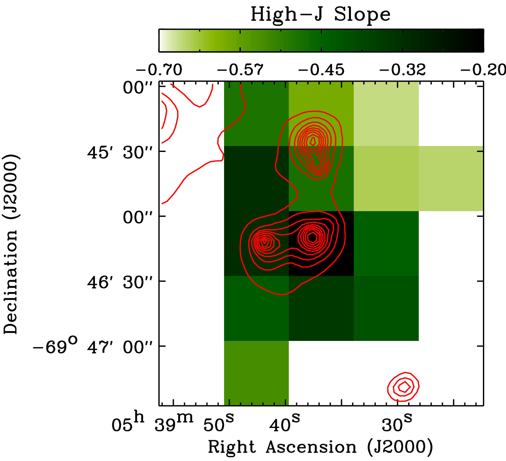
We present the observed CO SLEDs from = 1 to 13 ( = 2 not included) in Figure 8. To construct the CO SLED on a pixel-by-pixel basis, we use the integrated intensity images smoothed to the common resolution of 42′′ and apply a threshold of S/Ns > 5 for line detection. Our CO SLED image clearly shows regional variations in the shape of the CO SLEDs, indicating different physical conditions of the CO-emitting gas. For example, the location of the peak and the slope beyond the peak are sensitive to the density and temperature, while the CO column density determines the line intensity magnitude. In N159W, most of the observed CO SLEDs peak at 6 (gray in Figure 8; 10 pixels at = 6 and 1 pixel at = 7), while some show peaks that are uncertain due to non-detections (red; 2 pixels) or occur at the transitions lower than = 6 (green; 1 pixel at = 5 and 2 pixels at = 4). It is interesting to notice that the CO SLEDs with peaks at 5 are all located at the edge of our FTS maps, some distance away from the active star-forming regions. In addition, the slope of each CO SLED beyond its peak spatially changes. To quantify how different the slopes are, we compute the “high- slope” by = () ()/(), where () is the integrated intensity of the peak transition and () is the integrated intensity of the transition (Figure 9). By definition, the high- slope is always negative and a smaller value represents a steeper decrease. The transition is chosen here to calculate the high- slope for all pixels except for those two whose peaks are uncertain. We find that the high- slope changes by a factor of 3 across N159W. In particular, the two pixels corresponding to the active star-forming regions at (R.A.,decl.) (05h39m40s,46′10′′) (traced by the Spitzer 24 m emission in Figure 9) have the flattest CO SLEDs with 0.3 while the pixels at the northwest edge of our FTS maps show the steepest decrease with 0.7. A similar approach was recently adopted in Rosenberg et al. (2015), where the parameter = (=11–10) + (=12–11) + (=13–12)/ (=5–4) + (=6–5) + (=7–6) was used to categorize the CO SLEDs of 29 (ultra)luminous infrared galaxies ((U)LIRGs). Almost an order of magnitude variation in the parameter was found, confirming the diverse CO SLEDs found for many Galactic and extragalactic sources (e.g., Habart et al. 2010; van der Werf et al. 2010; Köhler et al. 2014; Kamenetzky et al. 2014; Mashian et al. 2015).
4.2 Non-LTE Modelling
We analyze the observed CO SLEDs using the non-LTE radiative transfer code RADEX (van der Tak et al. 2007). To compute the intensities of atomic and molecular lines, RADEX solves the radiative transfer equation based on the escape probability method. By assuming that the spectral lines are produced in an isothermal and homogeneous medium, this simple model can then be used to constrain the physical conditions of the medium, e.g., kinetic temperature, density, and column density of each species.
To model the intensity of each CO transition, we consider a grid of the following input parameters: kinetic temperature = 10–103 K, H2 density = 102–105 cm-3, CO column density (CO) = 1015–1020 cm-2, and beam filling factor = 10-3–1. These input parameters are sampled uniformly in log space with 50 points, except for (CO) where 100 points are used. In addition, we use the cosmic microwave background radiation temperature of 2.73 K and the FWHM linewidth of 10 km s-1 (based on Pineda et al. (2008) and Mizuno et al. (2010), where CO transitions up to =7–6 were spectrally resolved for N159W). In our modelling, we compare the observed integrated intensities () with RADEX predictions scaled by the beam filling factor () and find the best-fit model with the minimum where is defined as
| (1) |
Here is the uncertainty in the observed integrated intensity and the summation is done for the CO transitions from = 1 to 13 ( = 2 not included) with S/Ns > 5. We start with fitting the CO lines with a single temperature component, which is simplistic considering that multiple ISM phases are likely mixed at our spatial resolution of 10 pc. Nevertheless, using one component would still provide average physical conditions of the phases in the beam.


| Parameter | Minimum | Maximum | Median | |||
|---|---|---|---|---|---|---|
| All | Sub | All | Sub | All | Sub | |
| (K)a | 153 | 49 | 754 | 569 | 429 | 153 |
| (103 cm-3)a | 1.1 | 1.9 | 4.5 | 32.4 | 2.2 | 4.5 |
| (CO) (1017 cm-2)a | 0.4 | 0.9 | 10.7 | 13.5 | 3.4 | 7.6 |
| (10-1)a | 0.2 | 0.2 | 4.9 | 2.4 | 1.4 | 0.9 |
| (105 K cm-3)b | 3.6 | 3.6 | 12.6 | 16.0 | 9.5 | 8.7 |
| <> (1016 cm-2)b | 1.6 | 2.0 | 5.6 | 8.9 | 3.0 | 4.0 |
We determine the best-fit RADEX models for individual pixels and show them with the observed CO SLEDs in Figure 8. To illustrate how to estimate the uncertainties in the best-fit parameters, we then show the histograms of “good” parameters for the central pixel of our FTS maps ( in Figure 8) in Figure 10. To derive these histograms, we apply a threshold of minimum + 4.7 to the calculated distribution: = 4.7 is chosen for the 1 confidence interval with four parameters (, (H2), (CO), and ; Press et al. 1992). In addition to the histograms of the four primary parameters, those of secondary parameters, thermal pressure = (H2) and beam-averaged CO column density <> = (CO), are presented. We calculate the upper and lower error bounds by measuring the standard deviation of each “good” parameter distribution in log space, while noting that the distributions of “good” parameters are not always symmetric around the best-fit values. Since the primary parameters are degenerate in our modelling ( with and (CO) with )55 5 Higher temperatures and lower densities can produce the same intensity as lower temperatures and higher densities. The same thing applies to CO column densities and beam filling factors., their products, and <>, are better constrained in general. The images of the best-fit parameters are presented in Figure 11 and their ranges and 1 uncertainties are summarized in Table 2.
4.3 Spatial Distributions of the Best-fit Parameters
Figure 11 shows how the properties of the CO-emitting gas vary across N159W. We summarize our findings as follows.
Primary parameters: and (H2) show quite uniform distributions (only a factor of 2 variations around the median values of 429 K and 2.2 103 cm-3), while (CO) and change by a factor of 30 across the entire 40 pc 40 pc region. For example, varies from 0.02 to 0.5, but again mostly around the median of 0.1 (Figure 11). The estimated beam filling factor of 0.1 suggests that the CO clumps in N159W are on average 9′′ in size (2 pc at the LMC distance). This is consistent with what high-resolution ALMA observations of 13CO(1–0), 13CO(2–1), and 12CO(2–1) in N159W found (Fukui et al. 2015): the spatially resolved CO structures are roughly 10′′ in size.
An interesting trend is that the pixels with high kinetic temperatures (500–754 K) and beam filling factors (0.1–0.2) coincide with the data points with the flattest CO SLEDs (Figure 9), essentially tracing the massive star-forming regions. On the other hand, the CO column density distribution shows the opposite: the peak ((0.6–1) 1018 cm-2) instead occurs at the southeast and northwest edges of our FTS coverage. We note, however, that the primary parameters are degenerate in our RADEX modelling and have relatively large 1 uncertainties (e.g., Table 2), limiting our ability to examine the spatial distributions of the parameters more accurately.
Secondary parameters: Since the primary parameters are not independent of each other, it is therefore their products that can be better constrained and interpreted more straightforwardly. We find that both the thermal pressure and beam-averaged CO column density distributions are quite uniform with only a factor of 4 variations over our whole coverage. Their median values are 9.5 105 K cm-3 and 3.0 1016 cm-2 respectively.
Conclusion: The excellent agreement between the RADEX models and our CO SLEDs (Figure 8) suggests that the CO lines up to =12–11 observed on 10 pc scales are on average produced by a single temperature component. Our modelling shows that this component can be characterized by high thermal pressures of 9.5 105 K cm-3 and moderate beam-averaged CO column densities of 3.0 1016 cm-2 whose distributions are uniform across the 40 pc 40 pc region. Considering the good fit with the single temperature component, we do not attempt to add extra components in our RADEX modelling, since it would then introduce additional uncertainties, e.g., how different components are mixed and contribute to each CO transition. One component fitting has been done for both Galactic (e.g., Köhler et al. 2014) and extragalactic (e.g., Meijerink et al. 2013; Wu et al. 2015b) sources, while multiple components (up to three) have been used only in those cases where a single component clearly fails to reproduce the full CO SLEDs (e.g., Rangwala et al. 2011; Kamenetzky et al. 2012; Pellegrini et al. 2013; Israel et al. 2014; Kamenetzky et al. 2014; Papadopoulos et al. 2014; Rosenberg et al. 2014; Stock et al. 2015). In Section 5.4, however, we discuss the possible presence of a second component in the context of the origin of the CO emission.
4.4 Other General Properties
In this section, we discuss several of the general properties deduced from RADEX modelling.
Sub-thermalized CO: The average H2 densities of (H2) 2.2 103 cm-3 are much lower than the critical densities of 104–106 cm-3 (Table 1; Yang et al. 2010), suggesting that the FTS CO lines are sub-thermalized in N159W. In the optically thin case, their intensities depend on the kinetic temperature and density squared. For optically thick lines, the CO column density mainly determines the intensity. In our RADEX modelling, CO lines with = 3, 4, 5, and 6 are generally optically thick with 1 10.
High ratio of the CO to dust temperatures: We find that the CO and dust temperatures have generally similar distributions (Spearman’s rank correlation coefficient of 0.8): both peak at the location of the main star-forming regions, (R.A.,decl.) (05h39m40s,46′10′′), and decrease toward the edge of our FTS coverage. An absolute comparison, however, shows that the dust temperature is always lower than the CO temperature with a narrow range of 25–33 K. In the ISM, gas and dust are not in thermodynamical equilibrium, except for very dense ((H2) 106 cm-3) regions where the gas and dust temperatures become comparable due to the strong gas-dust coupling (e.g., Goldsmith 2001). The relatively uniform dust temperature results in a wide range of / 6–24. On average, the CO-to-dust temperature ratio is high with 14 being the median value and this is reflected in the unusually high / of 8 10-4 for N159W, which could hint at shock excitation (Section 5.3.4 for details).
Impact of the warm molecular gas on the surrounding ISM: The CO-emitting gas in N159W is almost isobaric with the thermal pressure of 9.5 105 K cm-3, which seems high enough to be important for the dynamics of HII regions. Recently, Lopez et al. (2014) measured several types of pressures exerted on the shells of 32 HII regions in the Magellanic Clouds (N159W not included) by analyzing radio, IR, optical, UV, and X-ray observations. These pressures were associated with direct stellar radiation, dust-processed IR radiation, warm ionized gas, and hot X-ray gas and the authors found that the warm ionized gas generally dominates over the other terms with the thermal pressure of (1–10) 106 K cm-3. The pressure of the CO-emitting gas in N159W is indeed comparable with the warm ionized gas pressure, suggesting that the energy and momentum associated with the warm CO could also play a significant role in the evolution of HII regions.

| Parameter | Locationa | This Work | Nikolić07d | Pineda08e | Mizuno10f | |
|---|---|---|---|---|---|---|
| Allb | Subc | |||||
| (K) | [0,2] | 324 | 72 | 15–95 | ||
| [0,1] | 471 | 126 | 80 | 70 | ||
| (103 cm-3) | [0,2] | 2.9 | 16.0 | 10 | ||
| [0,1] | 2.2 | 7.9 | 10 | 4 | ||
| (CO) (1017 cm-2) | [0,2] | 3.4 | 8.5 | 6–12 | ||
| [0,1] | 2.7 | 8.5 | 10g | 35 | ||
| (10-1) | [0,2] | 1.6 | 1.0 | 0.9–7.0 | ||
| [0,1] | 2.1 | 1.0 | 2 | |||
a Pixel location (Figure 8).
0,2 and 0,1 correspond to (05h39m36.8s,45′12.6′′) and
(05h39m36.8s,45′42.6′′).
b “All”: RADEX solutions determined using all available CO transitions (Section 4.2).
c “Sub”: RADEX solutions for CO transitions only up to =7–6 (Section 4.5).
d CO(1–0), CO(2–1), CO(3–2), 13CO(1–0), and 13CO(2–1) lines were modelled with the non-LTE radiative transfer model by Jansen et al. (1994).
e CO ( = 1, 4, and 7), 13CO ( = 1 and 4), and CI (609 m and 370 m) transitions were analyzed
using the escape probability radiative transfer model by Stutzki & Winnewisser (1985).
f CO ( = 1, 2, 3, 4, and 7) and 13CO ( = 1, 2, 3, and 4) data were combined with
the large velocity gradient (LVG) model by Goldreich & Kwan (1974).
d,e,f All analyses were done on 45′′ scales.
g CO linewidth of 10 km s-1 is used for this estimate.
4.5 Comparison with Previous Studies
A number of authors have also studied the physical conditions of the CO-emitting gas in N159W (e.g., Bolatto et al. 2005; Nikolić et al. 2007; Pineda et al. 2008; Minamidani et al. 2008; Mizuno et al. 2010). In this section, we compare our results with three of the most recent high-resolution studies: Nikolić et al. (2007), Pineda et al. (2008), and Mizuno et al. (2010). These studies analyzed mainly CO (up to =7–6) and 13CO (up to =4–3) transitions using various radiative transfer models and their results on 45′′ scales are presented in Table 3. To make a comparison, we list our RADEX results for the pixels that are the closest to the pointings analyzed in the previous studies (“All” in Table 3).
The comparison between our work and the previous studies shows a large difference, particularly in and (CO): we estimate a much higher (300–500 K vs. 100 K) and a much lower (CO) (3 1017 cm-2 vs. (10–40) 1017 cm-2). This large discrepancy most likely arises from the fact that high- CO transitions are included in our study and we test this hypothesis by performing RADEX modelling following what we do in Section 4.2 but using CO lines only up to CO(7–6) (the highest transition in the previous studies). The best-fit models are shown in Figure 12 and are summarized in Tables 2 and 3 (“Sub”).
As shown in Figure 12, a single temperature component fits the CO SLEDs quite well up to =7–6 but deviates from =8–7. Excluding high- CO transitions affects all RADEX parameters, particularly , (H2), and (CO). The re-derived is much lower than what we estimate in Section 4.2, while (H2) and (CO) increase in our re-modelling. The secondary parameters, and <(CO)>, and the beam filling factor are relatively less affected. We find that the new parameters are indeed in reasonably good agreement with the results from the previous studies (Table 3). Limiting the number of CO transitions, however, substantially increases the uncertainties in RADEX modelling and our original and newly-derived parameters are in fact consistent within 1 errors except for . Even for , only 3 out of the total 16 pixels show statistically significant differences. All these results suggest that including high- lines (beyond the CO SLED peak transition) is critical to characterize the physical conditions of CO emission with better accuracy.

5 Heating Sources in N159W
To understand the origin of the warm CO in N159W, we consider four primary heating sources: UV photons, X-rays, cosmic-rays, and mechanical heating.
5.1 UV Photons and X-rays
As one of the active star-forming regions in the LMC, N159W harbors massive stars whose intense UV radiation fields have a significant impact on the chemical and thermal structures of the ISM. Figure 13 shows the locations of such UV sources (massive YSOs from Chen et al. 2010 and OB stars from Fariña et al. 2009) on the integrated intensity image of CO(6–5), the transition where most of the observed CO SLEDs peak (Section 4.1). Other than UV photons, X-rays from the nearby LMC X-1, the most powerful X-ray source in the LMC (Section 1; black cross on Figure 13), could be another important source of heating. To probe the impact of UV and X-ray photons on the CO emission in N159W, we perform PDR modelling using an updated version of the Meudon PDR code (version 1.6; Le Petit et al. 2006). The major updates relevant for the present study are the implementation of (1) X-ray physics and (2) photo-electric heating based on the prescription by Weingartner & Draine (2001) and Weingartner et al. (2006) instead of Bakes & Tielens (1994). These updates will be presented in a forthcoming paper (B. Godard et al., in prep.). Finally, the formation rate of H2 is modelled considering the Eley-Rideal and Langmuir-Hinshelwood mechanisms as described in Le Bourlot et al. (2012). For computing time reason, we do not use the most sophisticated model of H2 formation that considers random fluctuations in the dust temperature (Bron et al. 2014).


5.1.1 Meudon PDR Modelling
The Meudon PDR code is a one-dimensional plane-parallel PDR model with one- or two-sided illumination. The model computes the distributions of atomic and molecular species for a slab of gas and dust based on thermal and chemical balance. For details on the chemical and physical processes and numerical computations in the model, we refer the reader to Le Petit et al. (2006).
In our analysis, each of the data points is modelled as a single cloud with a constant thermal pressure , irradiated by a radiation field on two sides. The radiation field has the spectral shape of the interstellar radiation field in the solar neighborhood (Mathis et al. 1983) and its intensity varies with the scaling factor . = 1 corresponds to the integrated energy density of 6.8 10-14 erg cm-3 for 5–13.6 eV. To consider a range of the physical conditions in N159W, a large parameter space of / = (3–3000) 104 K cm-3 and = 10–105 is examined. For two-sided illumination, the varied = 10–105 is incident on only one side, while the fixed = 1 is used for the other side. Other important model parameters include: metallicity , PAH-to-dust mass ratio , -band dust extinction (as a measure of the cloud size), X-ray flux , and cosmic-ray ionization rate . For N159W, = 0.5 and = 2% (constrained by dust SED modelling; Section 2.4) are adopted and a range of values, 0.5, 1, 3, 5, and 10 mag, are tested. To evaluate the impact of X-rays from LMC X-1, two values of = 0 and 10 are then explored ( = 1 corresponds to the integrated energy density of 5.3 10-14 erg cm-3 for 0.2–10 keV). The second value of = 10 is chosen to be the maximum incident X-ray flux we expect for the case where there is no absorption between LMC X-1 and N159W. Consequently, the influence of X-rays is in reality most likely weaker than the = 10 case. As for , the typical value of 3 10-16 s-1 for the diffuse ISM (e.g., Indriolo & McCall 2012) is adopted for the model. Finally, line opacities and intensities are calculated assuming the Doppler broadening of ()1/2, where = ()1/2 is the thermal linewidth ( = mass of the atomic/molecular species) and is the microturbulent linewidth (3.5 km s-1 is adopted in our study).
Our approach for PDR modelling is first to constrain and by comparing the observed line ratios of (OI 145 m + CII 158 m)/FIR luminosity, OI 145 m/CII 158 m, and CII 158 m/CI 370 m with model predictions and then to see if the constrained conditions reproduce the measured CO intensities. For our purpose, the PACS and dust data presented in Sections 2.2 and 2.4 are combined with the ground-based and FTS CO observations. All data sets are smoothed to 42′′ resolution and cast onto the common grid, resulting in five pixels to work with (outlined in green in Figure 13). The five pixels correspond to the main star-forming regions of N159W and this small number of pixels available for our PDR analysis is primarily due to the limited coverage of the PACS images (e.g., Figure 4). Finally, we note that the OI 63 m line is not included in our analysis due to the likely effect of high optical depth. The observed ratio of OI 145 m/OI 63 m is 0.1 over all five pixels, possibly indicating that the OI 63 m transition is optically thick (e.g., Tielens & Hollenbach 1985).
5.1.2 Results
Our PDR modelling is done for all five pixels and we summarize overall findings in this section. The results for one pixel (shown with the green star in Figure 13; 10 pc size) are presented in Figure 14 just as an illustration. First of all, we find that the observed three line ratios are well reproduced by the models with = 0.5 mag. For the models with 0.5 mag, the CII 158 m/CI 370 m ratio does not converge with the other two line ratios (this divergence becomes greater with increasing ), as shown in the bottom panels of Figure 14 for = 1 mag. The best-fit parameters (determined as having the minimum ) for the PDR model with = 0.5 mag and = 0 are (5–20) 105 K cm-3 and 70–120 across all five pixels. Other than and , we can also constrain the beam filling factor 5–7 by comparing the observed CII 158 m intensity with the predicted value. Using other tracers (e.g., OI 145 m and CI 370 m) results in essentially the same beam filling factors and 1 suggests that multiple components exist along each line of sight. In fact, 5–7 clouds whose individual is 0.5 mag are indeed in agreement with what we measure from dust SED modelling, 2–3 mag (probing the total dust abundance along the whole line of sight; Section 2.4). Finally, we find that the best-fit parameters for the models with = 0 and = 10 are comparable, implying that X-rays from the nearby LMC X-1 do not make a significant impact on the PDR tracers used in our analysis.
Now we investigate whether the constrained PDR conditions reproduce the ground-based and FTS CO observations. First, we compare the best-fit PDR solutions with our RADEX modelling results (Section 4.2) and find that the beam filling factor of the PDR tracers is a factor of 40 larger than that of the CO lines, while the constrained pressure is in agreement. This large difference in the beam filling factor could indicate that most of the CO emission in N159W does not originate from PDRs, where UV photons determine the thermal and chemical structures of the ISM. In addition, the kinetic temperature of 70 K for the CO-emitting gas in the PDR model is lower than what we estimate for the CO lines via RADEX modelling (320–750 K for the five pixels in our PDR analysis). The lower kinetic temperature has a substantial influence on CO emission and we indeed find that the predicted CO SLEDs are much fainter than the observed ones, as clearly shown in the top panels of Figure 15. The discrepancy in the CO integrated intensity becomes greater with increasing , e.g., from a factor of 540–950 for CO(1–0) to a factor of (2.9–8.3) 104 for CO(12–11) ( = 0.5 mag and = 0 case), and is particularly significant for the three pixels around the CO(6–5) peak (marked with the green star and circles in Figure 13). In terms of the total CO integrated intensity (CO transitions from =1–0 to =12–11 are summed; =2–1 excluded), the PDR model underestimates by a factor of a few (102–103). The shape of the observed CO SLEDs is also not reproduced by the PDR model. For example, the predicted CO SLEDs peak at either =4–3 or =5–4, while most of the observed CO SLEDs have a peak at =6–5 (e.g., Figure 8). In addition, the predicted CO SLEDs decrease beyond the peaks more steeply than what we measure in N159W, e.g., the ratio of CO(12–11) to CO(6–5) is 0.2–0.4 in the observations, while (0.5–1.2) 10-2 in the PDR model ( = 0.5 mag and = 0 case). The failure of the PDR model to reproduce the shape of the observed CO SLEDs is also clearly shown in the middle panels of Figure 15, where the three CO line ratios, CO(3–2)/CO(1–0), CO(6–5)/CO(3–2), and CO(9–8)/CO(6–5), do not converge to one solution over all parameter space. While the discrepancy we described so far is for the PDR model with = 0.5 mag and = 0, the presence of X-rays only slightly reduces the discrepancy (by only a factor of 2–5 in the case of the total CO integrated intensity). Finally, we note that the PDR models with higher values (up to 10 mag) still do not reproduce the observed CO(3–2)/CO(1–0), CO(6–5)/CO(3–2), and CO(9–8)/CO(6–5) ratios. To illustrate this result, PDR modelling with = 3 mag is presented in the bottom panels of Figure 15. Essentially, as increases, the three CO line ratios go upward in the vs. plot, but never converge to one solution.
Summary: Our modelling of the OI 145 m, CII 158 m, CI 370 m, and FIR data suggests that the PDR component in the main star-forming regions of N159W has the thermal pressure 106 K cm-3 and the incident UV radiation field 100. The CO emission originating from this PDR component is very weak and X-rays make only a minor difference. The majority of the observed CO emission (at least over the 264 pc2 region in our PDR analysis), therefore, must be excited by something other than UV photons and X-rays.
5.2 Cosmic-rays
Low-energy cosmic-rays ( 1–10 MeV) are another important source of heating in the ISM. Cosmic-rays ionize atoms and molecules in collision and the substantial kinetic energy of the resulting primary electrons goes into gas heating (35 eV and 6 eV for the ionized and neutral medium respectively) through secondary ionization or excitation of atoms and molecules (e.g., Grenier et al. 2015). To evaluate the impact of cosmic-rays on the FIR fine-structure and CO lines, we examine one Meudon PDR model with an increased cosmic-ray ionization rate of = 3 10-15 s-1, which is 10 times higher than the typical value we use in Section 5.1.1. This particular PDR model has = 0.5 mag, = 106 K cm-3, = 102, and = 10, the model parameters that well reproduce the observed FIR line ratios. Note that there is only a negligible difference between the PDR models with = 0 and 10. Our examination then reveals that the increased barely affects the FIR fine-structure and CO lines. To be specific, the OI 145 m, CII 158 m, and CI 370 m lines change by 4% at most, while the CO lines (up to =13–12) vary by a factor of 2.
Our exercise with the Meudon PDR model suggests that should be much higher than 3 10-15 s-1 to explain the discrepancy between the PDR model and the CO observations (Section 5.1.2). To quantify the cosmic-ray ionization rate that is required to fully reconcile the discrepancy, we then probe thermal balance in the regions analyzed with the PDR model (Figure 13).
Cooling: For the molecular medium with the warm temperature of 150–750 K and the intermediate density of a few 103 cm-3 (Table 2), H2 is one of the primary coolants (e.g., Neufeld et al. 1995; Kaufman & Neufeld 1996). Based on the calculation of H2 cooling function by Le Bourlot et al. (1999), we find the H2 cooling rate of 10-23–10-22 erg s-1 per molecule. For this estimate, we use the RADEX-based kinetic temperature and ortho-to-para ratio (Section 4.2) and consider two atomic-to-molecular hydrogen ratios, (H0)/(H2) = 10-2 and 1, the values suggested by Le Bourlot et al. (1999) for shocked-outflow and PDR conditions.
Heating: Heating by cosmic-rays can be estimated as (e.g., Wolfire et al. 1995)
| (2) |
where = energy deposited as heat by a primary electron and = (H0) + 2(H2). To derive the cosmic-ray heating rate, we use = 6 eV (appropriate for the neutral medium) and the RADEX-based H2 density (Section 4.2). In addition, we explore two values of (H0)/(H2) = 10-2 and 1, following our estimation of the cooling rate.
Thermal balance: By equating the heating and cooling rates, we are then able to derive 3 10-13 s-1, the cosmic-ray ionization rate that would fully account for the heating of the warm molecular medium in N159W. This estimate is a factor of 1000 higher than the typical value for the diffuse ISM. Fermi observations of the LMC recently showed that the -ray emissivity in the N159W region is roughly 10-26 ph s-1 sr-1 per hydrogen atom at most (Abdo et al. 2010), which is comparable to the value measured for the local diffuse ISM in the Milky Way (Abdo et al. 2009). The cosmic-ray density in N159W is hence most likely not too different from the diffuse ISM value, ruling out cosmic-rays as the main energy source for the warm CO in the regions analyzed with the Meudon PDR model.
5.3 Mechanical Heating
Along with UV photons, X-rays, and cosmic-rays, which primarily arise from the microscopic processes in the ISM, the macroscopic motions of gas can be an important source of heating. For example, energetic events such as stellar explosions (novae and supernovae), stellar winds, expanding HII regions, and converging flows strongly perturb the surrounding ISM and drive shocks. The shocks then accelerate, compress, and heat the medium, effectively converting much of the injected mechanical energy into thermal energy.

5.3.1 Paris-Durham Shock Modelling
In this section, we evaluate the impact of mechanical heating in N159W by comparing the observed CO and fine-structure lines with predictions from the Paris-Durham shock code (Flower & Pineau des Forêts 2015). This code simulates one-dimensional stationary J- or C-type shocks and calculates the dynamical and chemical properties of a multi-fluid medium (neutrals and ions), including densities, temperatures, velocities, and chemical abundances. For our study, we use the modified version by Lesaffre et al. (2013), which enables us to model UV-irradiated shocks, and create a grid of models covering the following input parameters: pre-shock density = 104, 105, and 106 cm-3, magnetic field parameter = 1 (defined as (/G)/, where is the strength of the magnetic field transverse to the direction of shock propagation), metallicity = 1 Z⊙, UV radiation field = 0 and 1 (defined as a scaling factor with respect to the interstellar radiation field by Draine 1978), and shock velocity from 4 km s-1 to 20 km s-1 with 2 km s-1 steps. Given the input densities and magnetic field parameter, our model grid only contains stationary C-type shocks (e.g., Le Bourlot et al. 2002; Flower & Pineau des Forêts 2003). To compare with the observed CO SLEDs, we then employ a post-processing treatment based on the LVG approximation, following the method used in Gusdorf et al. (2012), Anderl et al. (2014), and Gusdorf et al. (2015). In our modelling, the effects of grain-grain interactions (e.g., Guillet et al. 2011; Anderl et al. 2013) are not considered, since these effects play an important role only for high density and shock velocity ( cm-3 and km s-1) cases. Finally, we note that reducing the input metallicity by a factor of 2 to match the LMC value (0.5 ; e.g., Pagel 2003) would not change our main results. While the impact of low metallicity on the propagation of shocks has not been comprehensively examined, our preliminary analysis suggests that the CO and fine-structure line intensities would be affected by less than a factor of 2 in a half solar metallicity environment (Appendix B). Shock models with < 1 Z⊙ are currently under development and we hence focus on solar metallicity models in this study.
5.3.2 Results: CO and Fine-structure Lines
A subset of the Paris-Durham shock models is presented in Figure 16 with the observed CO SLEDs. To take into account the effect of beam dilution, the RADEX-based beam filling factor is applied to the predicted intensities on a pixel-by-pixel basis. We find that the shock models with = 104 cm-3, = 0, and 6–14 km s-1 reproduce our observations relatively well. In these models, gas is initially shocked with Mach and Alfvénic Mach numbers of 40 and 5. For the CO-bright layers ( 2 mag), the temperatures reach up to 180 K and 800 K for = 6 km s-1 and 14 km s-1 respectively and the post-shock densities are intermediate with a few 104 cm-3, which are in reasonably good agreement with our RADEX-based estimates (Section 4.2). On the other hand, the same shock models significantly underestimate the CII 158 m, OI 63 m, and [OI] 145 m intensities by up to a factor of a few 106 for CII 158 m and a factor of a few 102 for OI 63 m and 145 m. Note that this discrepancy persists even if we make an extreme assumption of = 1, e.g., the fine-structure lines entirely fill the 42′′ beam. While the current analyses have several limitations (e.g., only a single shock is considered over a small parameter space and the model parameters are degenerate), our results clearly demonstrate that mechanical heating by shocks can reproduce the observed CO intensities. The shock contributions to the CII 158 m, OI 63 m, and 145 m transitions are small, however, and these fine-structure lines are therefore most likely heated by other sources, e.g., UV photons. This conclusion is consistent with our PDR modelling (Section 5.1.2), where the observed fine-structure line ratios are well reproduced by a single PDR component with 106 K cm-3 and 100.
5.3.3 Results: Energetics
We now study the shock energetics in N159W. Our method follows the procedure presented in Anderl et al. (2014) and Gusdorf et al. (2015), but for the shock parameters that reproduce our CO observations: = 104 cm-3, = 1, = 1 Z⊙, = 0, and 6–14 km s-1. In essence, the Paris-Durham shock code predicts the fluxes of mass, momentum, and energy and we derive the total mass, momentum, and energy per modelled position in N159W by adopting a reasonable estimate for the size of shocked regions. To be specific, we assume a cylindrical shape for the shocked regions along each line of sight and use a circle with a diameter of 30′′ (FTS pixel size; corresponding to 41.5 pc2 at the LMC distance) for the surface area. As for the line of sight depth, we choose it as the length a neutral particle travels for 105 years with a shock velocity of (e.g., 0.2 pc for the model with = 10 km s-1). This timescale of 105 years is the typical time needed for the shocked gas to return to equilibrium after the passage of a shock wave with the characteristics considered in our analysis, as well as a satisfactory upper limit on the age of shocks associated with star formation or supernova remnants (e.g., Wolszczan et al. 1991; Williams et al. 2006; André 2011). Finally, we use the RADEX-based beam filling factor of = 0.1 to scale the predicted energetics, a representative value for the shocked CO clumps in the FTS pixels (Table 2). Bearing the uncertainties in our calculations (e.g., the stationary and one-dimensional model and the simplified cylindrical geometry with the less-known timescale for shocks), we find the total mass of shocked gas per modelled position of (0.9–2) 103 M⊙, which is roughly the mass of small molecular clouds or a small fraction (1–10%) of the mass of typical molecular clouds in the Milky Way (e.g., Dobbs et al. 2014). The total momentum injected by shocks on each modelled position is of the order of (0.6–3) 104 M⊙ km s-1, which is 105 and 103 times higher than that found for the shocks associated with the BHR71 low-mass stellar outflow (Gusdorf et al. 2015) and the relatively old supernova remnant W44 (Anderl et al. 2014) respectively. This large difference in the total momentum mainly results from the fact that the mass of shocked gas is much higher in N159W. Finally, the total energy dissipated by shocks is (0.4–4) 1048 ergs, which can for instance be compared with the typical 1051 ergs released by one supernova explosion (e.g., Hartmann 1999). In our calculations, one of the most uncertain parameters is the timescale of shocks, which can be off from the current value of 105 years by an order of magnitude. Our energetics estimates would then need to be scaled accordingly.

5.3.4 Origin of Shocks
The reasonably good agreement with the Paris-Durham model suggests that shocks are most likely the dominant heating source for the warm CO in N159W. Then what can drive these shocks? There are a few candidates (Figure 17) and we discuss them here.
LMC X-1: Cooke et al. (2007) observed the filamentary nebula surrounding LMC X-1 (N159F; Henize 1956) in several optical lines (H, OI, NII, SII, ArIII, and HeI) and found that all emission lines show a bow shock morphology. This shock structure was seen 4 pc away from LMC X-1 and was attributed to a presently unobserved jet from LMC X-1 (black cross and arrow in Figure 17). The observed line ratios were analyzed using the radiative shock model by Hartigan et al. (1987) and the jet-driven shock velocity of 90 km s-1 was constrained.
SNR J0540.06944: Williams et al. (2000) examined the X-ray emission from SNR J0540.06944 (blue circle in Figure 17) using Chandra observations and found that the SNR has a thick-shelled structure (19 pc in diameter). The observed X-ray structure indicated that SNR J0540.06944 is undergoing Sedov-like expansion and the SNR-driven shock velocity of 240 km s-1 was estimated.
Protostellar outflows: Fukui et al. (2015) recently discovered two molecular outflows, N159W-N and N159W-S (red squares in Figure 17), from their ALMA CO(2–1) observations at 1′′ resolution. This was the first discovery of extragalactic protostellar outflows. The outflows were found to have a velocity span of 10–20 km s-1 and to be associated with two massive YSOs previously studied by Chen et al. (2010). Redshifted and blueshifted lobes were clearly found for N159W-S, while N159W-N shows a blueshifted lobe only. All observed lobes are less than 0.2 pc. Note, however, that the active star-forming region N159W likely contains more stellar outflows, which have not been resolved in previous observations due to a lack of proper spatial and spectral resolution.
Colliding filaments: Interestingly, N159W-S was found at the intersection of two filamentary clouds. The two filaments have a width of 0.5–1 pc and a length of 5–10 pc and are clearly separated based on their blueshifted and redshifted velocities. Fukui et al. (2015) hypothesized that the two filaments collided 0.1 Myr ago with a velocity of 8 km s-1 and triggered the formation of N159W-S. As recently demonstrated by Wu et al. (2015a); Wu et al. (2016) with magnetohydrodynamic simulations, cloud–cloud collisions can drive shocks into the ISM.
Large-scale bubbles: N159W appears to be associated with large-scale bubbles that are considered to be produced by stellar feedback. For example, Jones et al. (2005) proposed that several O-type stars formed at the center of N159 about 1–2 Myr ago, driving a bubble with a radius of 20 pc (pink circle in Figure 17). N159W is at the periphery of this wind-blown bubble. In addition, the systematic search of large HI structures in the LMC by Kim et al. (1999) showed that N159W is located along the western edge of SGS 19 (purple circle in Figure 17). This HI supergiant shell centered at (R.A.,decl.) = (05h41m27s,69∘22′23′′) has a radius of 380 pc and an expansion velocity of 25 km s-1 (Dawson et al. 2013). Several other HI supergiant shells (SGSs 12, 13, 15, 16, 17, 20, and 22) were found surrounding SGS 19 (Figure 1), which may indicate that SGS 19 formed by sequential star formation (Kim et al. 1999). The counterpart shell in H, LMC2 (brightest H SGS in the LMC; Book et al. 2008), was also identified and seen to be confined to the inner edge of SGS 19.
Milky Way–Magellanic Clouds interaction: While the interaction between the Milky Way and the Magellanic Clouds and its impact on the evolution of gas and stars are currently under debate (D’Onghia & Fox 2015), it is most likely that the tidal force and/or ram pressure are at work in the southeastern HI overdensity region in the LMC, where N159W is located (Figure 1). For example, this HI overdensity region corresponds to the leading edge toward the Milky Way halo and de Boer et al. (1998) indeed suggested that a large amount of neutral gas was built up as a result of ram pressure of the hot halo gas on the LMC. In addition, the HI overdensity region appears to be connected with the Magellanic Bridge that exists between the LMC and the SMC (e.g., Kim et al. 1998; Putman et al. 2003), hinting at its tidal origin (e.g., Bekki & Chiba 2007; Besla et al. 2012).
In favor of large-scale shocks: We note that the good agreement with the Paris-Durham model is found for every pixel in Figure 16, which implies that CO is shock-heated across the entire FTS coverage (40 pc 40 pc region). This conclusion is also consistent with the fact that all individual pixels in our analysis have / 10-4. The threshold of / 10-4 is the diagnostic for shocks proposed by Meijerink et al. (2013) based on extensive theoretical modelling of UV and X-ray dominated regions (PDRs and XDRs; Meijerink & Spaans 2005; Meijerink et al. 2007). Essentially, Meijerink et al. (2013) argued that star-forming regions and active galactic nuclei (AGNs) creating PDRs and XDRs heat both gas and dust. On the other hand, shocks do not heat dust as effectively as they do for gas. As a result, CO line-to-TIR continuum ratios are expected to be higher in shocks than in PDRs and XDRs. The measured / is indeed 8 10-4 for the entire N159W, which is comparable to that of other extragalactic sources where mechanical heating was found to be the dominant heating mechanism for CO (e.g., NGC 6240, NGC 1266, Arp 220, M82, and M83; Figure 18). However, the regions of the largest discrepancy with the PDR model (shown as the green star and circles in Figure 13) do not exactly correspond to the pixels with high / values: two other pixels with less discrepancy have higher /. This indicates that the diagnostic power of the -to- ratio needs further investigation.

In summary, while all the candidates we describe can trigger shocks, large-scale physical processes, e.g., powerful stellar winds and supernova explosions that created supergiant bubbles in the LMC and Milky-Way–Magellanic Clouds interactions, are likely the primary drivers of shocks that heat CO in N159W. To test this hypothesis and evaluate how pervasive shocks are in the LMC, multiple CO transitions should be systematically examined over the entire LMC along with other tracers of PDRs and shocks (e.g., FIR fine-structure lines, SiO transitions, etc.). In particular, direct shock tracers such as SiO emission would be critical to constrain the properties of shocks with better accuracy, breaking the model degeneracy.
5.4 Synthesized View
In this section, we provide a synthesized view of the CO and fine-structure lines in N159W. In essence, our PDR and shock modelling indicate the presence of two distinct components: low- and high-extinction media where UV photons and shocks control the thermal and chemical structures of gas respectively. The low-extinction component fills the entire 42′′ beam with 0.5 mag and several clouds of this kind exist along a line of sight providing the total extinction of a few magnitudes. The medium is primarily heated by UV photons up to 70 K and emits very weak CO emission as a consequence of the low temperature and the low CO abundance at 0.5 mag. On the other hand, [OI] 145 m, [CII] 158 m, and [CI] 370 m are bright, explaining the fine-structure line observations of N159W. The second high-extinction component has a much smaller beam filling factor of 0.1 and is shock-heated up to 800 K. This warm medium has 2 mag on average and could be further shielded against dissociating UV photons by the first low-extinction component and other possible pre-shock medium (whose existence can be hinted by the excess of low- CO emission for several pixels compared to the shock model predictions; e.g., [-2,-1] and [-2,0] in Figure 16). As a result, abundant CO molecules can form and survive, reproducing the CO observations of N159W. On the contrary, the [OI] 145 m, [CII] 158 m, and [CI] 370 m fine-structure lines are weak. The two components are roughly in pressure equilibrium with 106 K cm-3.
We note that this interpretation is also compatible with our RADEX modelling. While the two components exist in N159W, the low-extinction, relatively cold one produces little CO emission (mainly at 4). On the other hand, the high-extinction, shock-heated warm medium emits bright in CO. This picture is in agreement with Section 4.2, where we find that the observed CO SLEDs are well reproduced with a single warm component.
6 Conclusions
We present Herschel SPIRE FTS observations of N159W, one of the most active star-forming regions in the LMC. Along with other multiwavelength tracers of gas and dust, the FTS observations are analyzed to examine the physical properties and excitation conditions of molecular gas (42′′ scales; corresponding to 10 pc). Our main results can be summarized as follows.
- 1.
In our FTS observations, CO rotational lines with (upper level ) = 4–12 and CI (609 m and 370 m) and NII (205 m) fine-structure lines are detected across the star-forming region.
- 2.
Intermediate- (6 9) and high- ( 10) CO lines show more compact spatial distributions than low- ( 5) CO lines. To be specific, the measured full width at half maximum is 42′′–60′′ for the low- transitions, while < 42′′ for the intermediate- and high- transitions. The two CI transitions are as compact as the intermediate- CO transitions.
- 3.
Combined with ground-based CO(1–0) and CO(3–2) observations, the FTS CO data are used to construct CO SLEDs on a pixel-by-pixel basis. We find that the peak and slope of the observed CO SLEDs change across the region, implying spatial variations in the physical conditions of the CO-emitting gas.
- 4.
The observed CO SLEDs are modelled with the non-LTE radiative transfer code RADEX and the following parameters are constrained across N159W on 10 pc scales: kinetic temperature = 153–754 K, H2 density (H2) = (1.1–4.5) 103 cm-3, CO column density (CO) = (0.4–10.7) 1017 cm-2, beam filling factor = 0.02–0.5, thermal pressure = (3.6–12.6) 105 K cm-3, and beam-averaged CO column density <(CO)> = (1.6–5.6) 1016 cm-2.
- 5.
We find that excluding CO transitions with > 7 affects all RADEX parameters, in particular , (H2), and (CO) ( underestimated and (H2) and (CO) overestimated along with larger 1 uncertainties, compared to the case where CO transitions up to = 12–11 are modelled). This suggests that high- lines (beyond the SLED peak transition) are crucial to quantify the physical properties of CO-traced molecular gas more accurately.
- 6.
While constraining the properties of PDRs traced by [OI] 145 m, [CII] 158 m, CI 370 m, and far-infrared luminosity (dust extinction 0.5 mag, thermal pressure 106 K cm-3, and incident UV radiation field 100 in the Mathis field units), the Meudon PDR model used in our analysis fails to explain the CO observations. Specifically, both the ampltitude and slope of the observed CO SLEDs are not reproduced, suggesting that the CO-emitting gas in N159W must be excited by something other than UV photons.
- 7.
X-rays from LMC X-1, the most strong X-ray source in the LMC, are found to have only a minor contribution to the CO emission. In addition, cosmic-rays are most likely not abundant enough to reproduce the observed warm CO, ruling out X-rays and cosmic-rays as the dominant heating source for CO in N159W.
- 8.
While only a limited parameter space is searched, our shock modelling with the Paris-Durham code clearly demonstrates that shocks can produce enough energy to excite the warm CO in N159W. On the other hand, the same shocks are faint in CII 158 m, OI 63 m, and 145 m. Several sources are considered as possible shock drivers and large-scale processes involving powerful stellar winds and supernova explosions that carved supergiant shells in the LMC and Milky Way–Magellanic Clouds interactions are likely the primary energy source for CO.
Our study of N159W in the LMC adds further evidence that the warm molecular medium is pervasive and CO rotational transitions are powerful diagnostic tools to probe the physical conditions of the medium. CO lines alone, however, have proven to be insufficient to pin down the origin of this warm molecular component in the ISM and additional tracers have been found to be critical for the analysis. For example, our Meudon PDR modelling shows that FIR fine-structure lines are essential to evaluate the contribution of UV photons to CO heating. In addition, Rosenberg et al. (2014a); Rosenberg et al. (2014b) suggested that dense gas tracers such as HCN, HNC, and HCO+ can be used to differentiate between UV-driven heating and mechanical heating. Molecular ions like H2O+ and OH+ were found particularly valuable to examine X-ray/cosmic-ray-driven heating and chemistry (e.g., van der Werf et al. 2010; Spinoglio et al. 2012).
Our work also supports the emerging picture that mechanical heating plays an important role in the excitation of molecular gas. In general, however, the source of mechanical heating has not been well-constrained, mostly because previous studies have not had high enough angular and spectral resolutions to resolve the drivers of mechanical energy, e.g., stellar winds/outflows, supernova explosions, spiral waves, and galaxy interactions. Systematic studies of various atomic and molecular species at high spatial and spectral resolutions are crucial to probe the driver(s) of mechanical heating and the detailed processes of energy dissipation in the ISM (e.g., Herrera et al. 2012; Larson et al. 2015; Rangwala et al. 2015), which will be possible particularly with ALMA, NOEMA, and JWST.
Acknowledgements.
We would like to thank the anonymous referee for the constructive comments that improved this work. We also thank Julia Kamenetzky, Edward Polehampton, Eric Pellegrini, and Naseem Rangwala for helpful discussions on FTS data reduction and science. M.-Y.L. acknowledges support from the DIM ACAV of the Region Ile de France and the SYMPATICO grant (ANR-11-BS56-0023) of the French Agence Nationale de la Recherche. SH acknowledges financial support from DFG programme HO 5475/2-1. PACS has been developed by a consortium of institutes led by MPE (Germany) and including UVIE (Austria); KU Leuven, CSL, IMEC (Belgium); CEA, LAM (France); MPIA (Germany); INAF-IFSI/OAA/OAP/OAT, LENS, SISSA (Italy); IAC (Spain). This development has been supported by the funding agencies BMVIT (Austria), ESA-PRODEX (Belgium), CEA/CNES (France), DLR (Germany), ASI/INAF (Italy), and CICYT/MCYT (Spain). SPIRE has been developed by a consortium of institutes led by Cardiff University (UK) and including Univ. Lethbridge (Canada); NAOC (China); CEA, LAM (France); IFSI, Univ. Padua (Italy); IAC (Spain); Stockholm Observatory (Sweden); Imperial College London, RAL, UCL-MSSL, UKATC, Univ. Sussex (UK); and Caltech, JPL, NHSC, Univ. Colorado (USA). This development has been supported by national funding agencies: CSA (Canada); NAOC (China); CEA, CNES, CNRS (France); ASI (Italy); MCINN (Spain); SNSB (Sweden); STFC, UKSA (UK); and NASA (USA).References
- Abdo et al. (2009) Abdo, A. A., Ackermann, M., Ajello, M., et al. 2009, ApJ, 703, 1249
- Abdo et al. (2010) Abdo, A. A., Ackermann, M., Ajello, M., et al. 2010, A&A, 512, A7
- Anderl et al. (2013) Anderl, S., Guillet, V., Pineau des Forêts, G., & Flower, D. R. 2013, A&A, 556, A69
- Anderl et al. (2014) Anderl, S., Gusdorf, A., & Güsten, R. 2014, A&A, 569, A81
- André (2011) André, P. 2011, in Encyclopedia of Astrobiology, ed. M. Gargaud, R. Amils, J. C. Quintanilla, H. J. J. Cleaves II, W. M. Irvine, D. L. Pinti, & M. Viso (Springer Berlin Heidelberg), 1549–1553
- Bakes & Tielens (1994) Bakes, E. L. O. & Tielens, A. G. G. M. 1994, ApJ, 427, 822
- Bekki & Chiba (2007) Bekki, K. & Chiba, M. 2007, PASA, 24, 21
- Besla et al. (2012) Besla, G., Kallivayalil, N., Hernquist, L., et al. 2012, MNRAS, 421, 2109
- Bolatto et al. (2005) Bolatto, A. D., Israel, F. P., & Martin, C. L. 2005, ApJ, 633, 210
- Book et al. (2008) Book, L. G., Chu, Y.-H., & Gruendl, R. A. 2008, ApJS, 175, 165
- Bron et al. (2014) Bron, E., Le Bourlot, J., & Le Petit, F. 2014, A&A, 569, A100
- Carilli & Walter (2013) Carilli, C. L. & Walter, F. 2013, ARA&A, 51, 105
- Carlson et al. (2012) Carlson, L. R., Sewiło, M., Meixner, M., Romita, K. A., & Lawton, B. 2012, A&A, 542, A66
- Chen et al. (2010) Chen, C.-H. R., Indebetouw, R., Chu, Y.-H., et al. 2010, ApJ, 721, 1206
- Chu et al. (1997) Chu, Y.-H., Kennicutt, R. C., Snowden, S. L., et al. 1997, PASP, 109, 554
- Cooke et al. (2007) Cooke, R., Kuncic, Z., Sharp, R., & Bland-Hawthorn, J. 2007, ApJ, 667, L163
- Cormier et al. (2015) Cormier, D., Madden, S. C., Lebouteiller, V., et al. 2015, A&A, 578, A53
- Dawson et al. (2013) Dawson, J. R., McClure-Griffiths, N. M., Wong, T., et al. 2013, ApJ, 763, 56
- de Boer et al. (1998) de Boer, K. S., Braun, J. M., Vallenari, A., & Mebold, U. 1998, A&A, 329, L49
- de Graauw et al. (2010) de Graauw, T., Helmich, F. P., Phillips, T. G., et al. 2010, A&A, 518, L6
- Dobbs et al. (2014) Dobbs, C. L., Krumholz, M. R., Ballesteros-Paredes, J., et al. 2014, Protostars and Planets VI, 3
- D’Onghia & Fox (2015) D’Onghia, E. & Fox, A. J. 2015, ArXiv e-prints [arXiv:1511.05853]
- Draine (1978) Draine, B. T. 1978, ApJS, 36, 595
- Draine & Li (2007) Draine, B. T. & Li, A. 2007, ApJ, 657, 810
- Fariña et al. (2009) Fariña, C., Bosch, G. L., Morrell, N. I., Barbá, R. H., & Walborn, N. R. 2009, AJ, 138, 510
- Flower & Pineau des Forêts (2003) Flower, D. R. & Pineau des Forêts, G. 2003, MNRAS, 343, 390
- Flower & Pineau des Forêts (2015) Flower, D. R. & Pineau des Forêts, G. 2015, A&A, 578, A63
- Fukui et al. (2015) Fukui, Y., Harada, R., Tokuda, K., et al. 2015, ApJ, 807, L4
- Fukui et al. (1999) Fukui, Y., Mizuno, N., Yamaguchi, R., et al. 1999, PASJ, 51, 745
- Fulton et al. (2010) Fulton, T. R., Baluteau, J.-P., Bendo, G., et al. 2010, in Society of Photo-Optical Instrumentation Engineers (SPIE) Conference Series, Vol. 7731, Society of Photo-Optical Instrumentation Engineers (SPIE) Conference Series
- Galametz et al. (2013) Galametz, M., Hony, S., Galliano, F., et al. 2013, MNRAS, 431, 1596
- Galliano et al. (2011) Galliano, F., Hony, S., Bernard, J.-P., et al. 2011, A&A, 536, A88
- Goldreich & Kwan (1974) Goldreich, P. & Kwan, J. 1974, ApJ, 189, 441
- Goldsmith (2001) Goldsmith, P. F. 2001, ApJ, 557, 736
- Gordon et al. (2008) Gordon, K. D., Engelbracht, C. W., Rieke, G. H., et al. 2008, ApJ, 682, 336
- Grenier et al. (2015) Grenier, I. A., Black, J. H., & Strong, A. W. 2015, ARA&A, 53, 199
- Greve et al. (2014) Greve, T. R., Leonidaki, I., Xilouris, E. M., et al. 2014, ApJ, 794, 142
- Griffin et al. (2010) Griffin, M. J., Abergel, A., Abreu, A., et al. 2010, A&A, 518, L3
- Guillet et al. (2011) Guillet, V., Pineau Des Forêts, G., & Jones, A. P. 2011, A&A, 527, A123
- Gusdorf et al. (2012) Gusdorf, A., Anderl, S., Güsten, R., et al. 2012, A&A, 542, L19
- Gusdorf et al. (2015) Gusdorf, A., Riquelme, D., Anderl, S., et al. 2015, A&A, 575, A98
- Habart et al. (2010) Habart, E., Dartois, E., Abergel, A., et al. 2010, A&A, 518, L116
- Hailey-Dunsheath et al. (2012) Hailey-Dunsheath, S., Sturm, E., Fischer, J., et al. 2012, ApJ, 755, 57
- Hartigan et al. (1987) Hartigan, P., Raymond, J., & Hartmann, L. 1987, ApJ, 316, 323
- Hartmann (1999) Hartmann, D. H. 1999, Proceedings of the National Academy of Science, 96, 4752
- Henize (1956) Henize, K. G. 1956, ApJS, 2, 315
- Herrera et al. (2012) Herrera, C. N., Boulanger, F., Nesvadba, N. P. H., & Falgarone, E. 2012, A&A, 538, L9
- Hollenbach & Tielens (1997) Hollenbach, D. J. & Tielens, A. G. G. M. 1997, ARA&A, 35, 179
- Indriolo & McCall (2012) Indriolo, N. & McCall, B. J. 2012, ApJ, 745, 91
- Israel et al. (2014) Israel, F. P., Güsten, R., Meijerink, R., et al. 2014, A&A, 562, A96
- Jansen et al. (1994) Jansen, D. J., van Dishoeck, E. F., & Black, J. H. 1994, A&A, 282, 605
- Johansson et al. (1994) Johansson, L. E. B., Olofsson, H., Hjalmarson, A., Gredel, R., & Black, J. H. 1994, A&A, 291, 89
- Jones et al. (2005) Jones, T. J., Woodward, C. E., Boyer, M. L., Gehrz, R. D., & Polomski, E. 2005, ApJ, 620, 731
- Kamenetzky et al. (2012) Kamenetzky, J., Glenn, J., Rangwala, N., et al. 2012, ApJ, 753, 70
- Kamenetzky et al. (2014) Kamenetzky, J., Rangwala, N., Glenn, J., Maloney, P. R., & Conley, A. 2014, ApJ, 795, 174
- Kaufman & Neufeld (1996) Kaufman, M. J. & Neufeld, D. A. 1996, ApJ, 456, 611
- Kennicutt & Evans (2012) Kennicutt, R. C. & Evans, N. J. 2012, ARA&A, 50, 531
- Kim et al. (1999) Kim, S., Dopita, M. A., Staveley-Smith, L., & Bessell, M. S. 1999, AJ, 118, 2797
- Kim et al. (1998) Kim, S., Staveley-Smith, L., Dopita, M. A., et al. 1998, ApJ, 503, 674
- Köhler et al. (2014) Köhler, M., Habart, E., Arab, H., et al. 2014, A&A, 569, A109
- Larson et al. (2015) Larson, R. L., Evans, II, N. J., Green, J. D., & Yang, Y.-L. 2015, ApJ, 806, 70
- Launay & Roueff (1977) Launay, J. M. & Roueff, E. 1977, A&A, 56, 289
- Le Bourlot et al. (2012) Le Bourlot, J., Le Petit, F., Pinto, C., Roueff, E., & Roy, F. 2012, A&A, 541, A76
- Le Bourlot et al. (1999) Le Bourlot, J., Pineau des Forêts, G., & Flower, D. R. 1999, MNRAS, 305, 802
- Le Bourlot et al. (2002) Le Bourlot, J., Pineau des Forêts, G., Flower, D. R., & Cabrit, S. 2002, MNRAS, 332, 985
- Le Petit et al. (2006) Le Petit, F., Nehmé, C., Le Bourlot, J., & Roueff, E. 2006, ApJS, 164, 506
- Lebouteiller et al. (2012) Lebouteiller, V., Cormier, D., Madden, S. C., et al. 2012, A&A, 548, A91
- Lesaffre et al. (2013) Lesaffre, P., Pineau des Forêts, G., Godard, B., et al. 2013, A&A, 550, A106
- Lopez et al. (2014) Lopez, L. A., Krumholz, M. R., Bolatto, A. D., et al. 2014, ApJ, 795, 121
- Lu et al. (2014) Lu, N., Zhao, Y., Xu, C. K., et al. 2014, ApJ, 787, L23
- Makiwa et al. (2013) Makiwa, G., Naylor, D. A., Ferlet, M., et al. 2013, Appl. Opt., 52, 3864
- Mashian et al. (2015) Mashian, N., Sturm, E., Sternberg, A., et al. 2015, ApJ, 802, 81
- Mathis et al. (1983) Mathis, J. S., Mezger, P. G., & Panagia, N. 1983, A&A, 128, 212
- Meijerink et al. (2013) Meijerink, R., Kristensen, L. E., Weiß, A., et al. 2013, ApJ, 762, L16
- Meijerink & Spaans (2005) Meijerink, R. & Spaans, M. 2005, A&A, 436, 397
- Meijerink et al. (2007) Meijerink, R., Spaans, M., & Israel, F. P. 2007, A&A, 461, 793
- Meixner et al. (2006) Meixner, M., Gordon, K. D., Indebetouw, R., et al. 2006, AJ, 132, 2268
- Minamidani et al. (2008) Minamidani, T., Mizuno, N., Mizuno, Y., et al. 2008, ApJS, 175, 485
- Mizuno et al. (2001) Mizuno, N., Yamaguchi, R., Mizuno, A., et al. 2001, PASJ, 53, 971
- Mizuno et al. (2010) Mizuno, Y., Kawamura, A., Onishi, T., et al. 2010, PASJ, 62, 51
- Neufeld et al. (1995) Neufeld, D. A., Lepp, S., & Melnick, G. J. 1995, ApJS, 100, 132
- Nikolić et al. (2007) Nikolić, S., Garay, G., Rubio, M., & Johansson, L. E. B. 2007, A&A, 471, 561
- Okada et al. (2015) Okada, Y., Requena-Torres, M. A., Güsten, R., et al. 2015, A&A, 580, A54
- Ott (2010) Ott, S. 2010, in Astronomical Society of the Pacific Conference Series, Vol. 434, Astronomical Data Analysis Software and Systems XIX, ed. Y. Mizumoto, K.-I. Morita, & M. Ohishi, 139
- Pagel (2003) Pagel, B. E. J. 2003, in Astronomical Society of the Pacific Conference Series, Vol. 304, CNO in the Universe, ed. C. Charbonnel, D. Schaerer, & G. Meynet, 187
- Papadopoulos et al. (2014) Papadopoulos, P. P., Zhang, Z.-Y., Xilouris, E. M., et al. 2014, ApJ, 788, 153
- Pellegrini et al. (2013) Pellegrini, E. W., Smith, J. D., Wolfire, M. G., et al. 2013, ApJ, 779, L19
- Pietrzyński et al. (2013) Pietrzyński, G., Graczyk, D., Gieren, W., et al. 2013, Nature, 495, 76
- Pilbratt et al. (2010) Pilbratt, G. L., Riedinger, J. R., Passvogel, T., et al. 2010, A&A, 518, L1
- Pineda et al. (2008) Pineda, J. L., Mizuno, N., Stutzki, J., et al. 2008, A&A, 482, 197
- Poglitsch et al. (2010) Poglitsch, A., Waelkens, C., Geis, N., et al. 2010, A&A, 518, L2
- Pon et al. (2014) Pon, A., Johnstone, D., Kaufman, M. J., Caselli, P., & Plume, R. 2014, MNRAS, 445, 1508
- Press et al. (1992) Press, W. H., Teukolsky, S. A., Vetterling, W. T., & Flannery, B. P. 1992, Numerical recipes in FORTRAN. The art of scientific computing (Cambridge University Press)
- Putman et al. (2003) Putman, M. E., Staveley-Smith, L., Freeman, K. C., Gibson, B. K., & Barnes, D. G. 2003, ApJ, 586, 170
- Rangwala et al. (2011) Rangwala, N., Maloney, P. R., Glenn, J., et al. 2011, ApJ, 743, 94
- Rangwala et al. (2015) Rangwala, N., Maloney, P. R., Wilson, C. D., et al. 2015, ApJ, 806, 17
- Rigopoulou et al. (2013) Rigopoulou, D., Hurley, P. D., Swinyard, B. M., et al. 2013, MNRAS, 434, 2051
- Rosenberg et al. (2014a) Rosenberg, M. J. F., Kazandjian, M. V., van der Werf, P. P., et al. 2014a, A&A, 564, A126
- Rosenberg et al. (2014b) Rosenberg, M. J. F., Meijerink, R., Israel, F. P., et al. 2014b, A&A, 568, A90
- Rosenberg et al. (2015) Rosenberg, M. J. F., van der Werf, P. P., Aalto, S., et al. 2015, ApJ, 801, 72
- Schirm et al. (2014) Schirm, M. R. P., Wilson, C. D., Parkin, T. J., et al. 2014, ApJ, 781, 101
- Schlegel et al. (1994) Schlegel, E. M., Marshall, F. E., Mushotzky, R. F., et al. 1994, ApJ, 422, 243
- Seale et al. (2012) Seale, J. P., Looney, L. W., Wong, T., et al. 2012, ApJ, 751, 42
- Spinoglio et al. (2012) Spinoglio, L., Pereira-Santaella, M., Busquet, G., et al. 2012, ApJ, 758, 108
- Stock et al. (2015) Stock, D. J., Wolfire, M. G., Peeters, E., et al. 2015, A&A, 579, A67
- Stutzki & Winnewisser (1985) Stutzki, J. & Winnewisser, G. 1985, A&A, 144, 13
- Swinyard et al. (2010) Swinyard, B. M., Ade, P., Baluteau, J.-P., et al. 2010, A&A, 518, L4
- Tielens (2005) Tielens, A. G. G. M. 2005, The Physics and Chemistry of the Interstellar Medium (Cambridge University Press)
- Tielens & Hollenbach (1985) Tielens, A. G. G. M. & Hollenbach, D. 1985, ApJ, 291, 722
- van der Marel & Cioni (2001) van der Marel, R. P. & Cioni, M.-R. L. 2001, AJ, 122, 1807
- van der Tak et al. (2007) van der Tak, F. F. S., Black, J. H., Schöier, F. L., Jansen, D. J., & van Dishoeck, E. F. 2007, A&A, 468, 627
- van der Werf et al. (2010) van der Werf, P. P., Isaak, K. G., Meijerink, R., et al. 2010, A&A, 518, L42
- Walker et al. (2015) Walker, K. M., Song, L., Yang, B. H., et al. 2015, ApJ, 811, 27
- Weingartner & Draine (2001) Weingartner, J. C. & Draine, B. T. 2001, ApJS, 134, 263
- Weingartner et al. (2006) Weingartner, J. C., Draine, B. T., & Barr, D. K. 2006, ApJ, 645, 1188
- Williams et al. (2006) Williams, B. J., Borkowski, K. J., Reynolds, S. P., et al. 2006, ApJ, 652, L33
- Williams et al. (2000) Williams, R. M., Petre, R., Chu, Y.-H., & Chen, C.-H. R. 2000, ApJ, 536, L27
- Wolfire et al. (1995) Wolfire, M. G., Hollenbach, D., McKee, C. F., Tielens, A. G. G. M., & Bakes, E. L. O. 1995, ApJ, 443, 152
- Wolszczan et al. (1991) Wolszczan, A., Cordes, J. M., & Dewey, R. J. 1991, ApJ, 372, L99
- Wong et al. (2011) Wong, T., Hughes, A., Ott, J., et al. 2011, ApJS, 197, 16
- Wu et al. (2016) Wu, B., Tan, J. C., Nakamura, F., et al. 2016, ArXiv e-prints [arXiv:1606.01320]
- Wu et al. (2015a) Wu, B., Van Loo, S., Tan, J. C., & Bruderer, S. 2015a, ApJ, 811, 56
- Wu et al. (2015b) Wu, R., Madden, S. C., Galliano, F., et al. 2015b, A&A, 575, A88
- Yang et al. (2010) Yang, B., Stancil, P. C., Balakrishnan, N., & Forrey, R. C. 2010, ApJ, 718, 1062
Appendix A FTS CO, [CI], [NII] Integrated Intensity Images
We present the FTS CO, [CI], and [NII] integrated intensity images of N159W (Section 2.1.2 for details on how we derive these images). All images have a resolution of 42′′ (10 pc at the LMC distance) and a pixel size of 30′′. For CO(4–3) and CO(9–8), the first CO transitions in the SLW and SSW, the SLW and SSW arrays are shown as the blue and green crosses, except the central detectors for the first jiggle observation (SLWC3 and SSWD4) in yellow and orange. The spectra with S/Ns > 5 (“detections”) are overlaid in red, while those with S/Ns 5 (“non-detections”) are in blue. To show the -axis (in GHz) and -axis (in 10-18 W m-2 Hz-1 sr-1 except for CO(13–12), which is in 10-19 W m-2 Hz-1 sr-1) ranges, the spectrum of the pixel observed with SLWC3 and SSWD4 is presented in the bottom right corner of each figure. Finally, the 2′ unvignetted field-of-view for FTS observations is indicated as the black dashed circle.


Appendix B Paris-Durham Shock Models with Half Solar Metallicity
We present some of the results from the shock models with 0.5 Z⊙. To simulate the propagation of shocks in the half solar metallicity ISM, we run the Paris-Durham code as we do for 1 Z⊙, but with metal (C, N, O, Mg, Si, S, and Fe), grain, and PAH abundances reduced by half. The geometrical properties of grains and PAHs remain the same. For our test runs, the shock parameters that reproduce the CO observations of N159W are used (Section 5.3.2): = 104 cm-3, = 1, = 0, and = 6, 10, and 14 km s-1. Note that this is the first attempt to run the Paris-Durham code with < 1 Z⊙.
We find that the difference between the two models in terms of the CO (up to =13–12) and fine-structure line ([CII] 158 m, [OI] 63 m, and [OI] 145 m) intensities is less than a factor of 2 (e.g., Figure 21). This small difference arises from the fact that shocks have similar thermal structures in the 1 Z⊙ and 0.5 Z⊙ models. As a result, the difference in the line intensities primarily comes from the difference in atomic/molecular abundances (e.g., less than a factor of 2 for CO at CO-bright shocked layers).
