Statistical analysis of m/n = 2/1 locked and quasi-stationary modes with rotating precursors at DIII-D
Abstract
A database has been developed to study the evolution, the nonlinear effects on equilibria, and the disruptivity of locked and quasi-stationary modes with poloidal and toroidal mode numbers and at DIII-D. The analysis of 22,500 discharges shows that more than 18% of disruptions are due to locked or quasi-stationary modes with rotating precursors (not including born locked modes). A parameter formulated by the plasma internal inductance divided by the safety factor at 95% of the poloidal flux, , is found to exhibit predictive capability over whether a locked mode will cause a disruption or not, and does so up to hundreds of milliseconds before the disruption. Within 20 ms of the disruption, the shortest distance between the island separatrix and the unperturbed last closed flux surface, referred to as , performs comparably to in its ability to discriminate disruptive locked modes. Out of all parameters considered, also correlates best with the duration of the locked mode. Disruptivity following a locked mode as a function of the normalized beta, , is observed to peak at an intermediate value, and decrease for high values. The decrease is attributed to the correlation between and in the DIII-D operational space. Within 50 ms of a locked mode disruption, average behavior includes exponential growth of the perturbed field, which might be due to the 2/1 locked mode. Surprisingly, even assuming the aforementioned 2/1 growth, disruptivity following a locked mode shows little dependence on island width up to 20 ms before the disruption. Separately, greater deceleration of the rotating precursor is observed when the wall torque is large. At locking, modes are often observed to align at a particular phase, which is likely related to a residual error field. Timescales associated with the mode evolution are also studied and dictate the response times necessary for disruption avoidance and mitigation. Observations of the evolution of during a locked mode, the effects of poloidal beta on the saturated width, and the reduction in Shafranov shift during locking are also presented.
1 Introduction
Rotating and non-rotating ("locked") neoclassical tearing modes (NTMs) are known to degrade confinement and cause disruptions in tokamak plasmas under certain plasma conditions, and thus represent a concern for ITER [1].
NTMs can rotate at the local plasma rotation velocity, apart from a small offset of the order of the electron or ion diamagnetic velocity [2]. In present tokamaks with strong torque injection, this corresponds to rotation frequencies of several kHz. Magnetic islands can also steadily rotate at frequencies of the order of the inverse resistive-wall time (tens of Hz, typically), if a stable torque balance can be established at that frequency. In this case, they are called Quasi Stationary Modes (QSMs) [3].
There are also NTMs that do not rotate at all, called Locked Modes (LMs). Some of these are the result of an initially rotating NTM ("rotating precursor") decelerating and locking to the residual error field. The deceleration might be due to the magnetic braking experienced by the rotating island in its interaction with the eddy currents that it induces in the resistive wall [4]. Other modes are "born locked", i.e. they form without a rotating precursor, as a result of resonant error field penetration.
It will be important to understand the onset, growth, saturation, and stabilization of all these categories of rotating and non-rotating NTMs, in order to maintain good confinement and prevent disruptions in ITER. Here we present an extensive analysis of QSMs and LMs with rotating precursors, which we will sometimes refer to as "initially rotating locked modes", or IRLMs. The analysis was carried over approximately 22,500 DIII-D [5] plasma discharges, and restricted to poloidal/toroidal mode numbers m/n=2/1, because these are the mode numbers that are most detrimental to plasma confinement in DIII-D and most other tokamaks [6]. QSMs and LMs of different (for example 3/2, occasionally observed at DIII-D) and LMs not preceded by rotating precursors are not considered here and will be the subject of a separate work.
Previous works have described classical [7, 8] and neoclassical [9, 6, 10] tearing modes (TMs), and the torques acting on TMs [4]. Effects of TMs on confinement are described theoretically [11]. Summaries of error-field-penetration locked modes in DIII-D [12], disruption phenomenology in JET [13], and disruption observations across many machines [14] have been reported.
Statistics regarding the role of plasma equilibrium parameters, and MHD stability limits on disruptions have been reported at JET [15], and one work includes a detailed accounting of the instabilities preceding the disruptions [16]. A comprehensive study of disruptivity as a function of various equilibrium parameters was conducted at NSTX [17] followed by a work on disruption prediction including locked mode parameters [18]. A study of various disruption types on JT-60U, including those caused by tearing modes, has been reported [19]. A brief study of disruptivity as a function of the safety factor and the normalized plasma beta on DIII-D has been reported [20].
Machine learning approaches to disruption prediction have shown rather high levels of success at ASDEX Upgrade [21, 22], JET [23], and JT-60U [24], and a predictor tuned on JET was ported to ASDEX Upgrade [25]. Similarly, neural networks have been used for disruption prediction at TEXT [26], and ADITYA [27], and for predicting ideal stability boundaries on DIII-D [28]. Discriminant analysis for disruption prediction was tested at ASDEX Upgrade [29].
A statistical work on MAST investigated the differences between disruptive and non-disruptive LMs as a function of normalized plasma beta and the safety factor [30]. Recently a locked mode thermal quench threshold has been proposed based on equilibrium parameters from studies on JET, ASDEX Upgrade, and COMPASS [31]. The automatic detection of locked modes with rotating precursors makes the disruption statistics presented here unique. In addition, this work includes basic observations of locked modes and their effects on equilibria.
During the first discharges in this database, DIII-D was equipped with one poloidal and four toroidal arrays of Mirnov probes and saddle loops [33]. During the time spanned by the database, additional sensors were added for increased 3D resolution [34]. However, a limited set of six saddle loop sensors (external to the vessel) and three poloidal sensors (inside the vessel) are used for simplicity, and for consistency of the analysis across all shots, spanning the years 2005-2014.
An example of the 2/1 IRLMs considered here is illustrated in figure 1. The poloidal field amplitude of the rotating precursor is detected by the toroidal array of Mirnov probes around 1800 ms. The mode simultaneously grows and slows down until it locks at 1978.5 ms. Due to the finite time binning used in the Fourier analysis during the rotating phase, the rotating signal is lost at low frequency, and is instead measured by a set of large saddle loops (ESLDs: external saddle loops differenced). The response of the saddle loops increases when , where ms is the characteristic wall time for DIII-D. As shown in Fig.1, it is not uncommon for the amplitude of an IRLM to oscillate due to minor disruptions, and to grow prior to disruption (this will be investigated in section 6.2).
Three interesting results of this work are introduced now. First, it will be shown that the island width cannot be used to distinguish disruptive from non-disruptive IRLMs 20 ms or more ahead of the disruption time. Similarly, the island width shows little correlation with the IRLM survival time.
Second, the plasma internal inductance divided by the safety factor, , distinguishes IRLMs that will disrupt from those that will not. The predictive capability of might be related to the energy available to drive nonlinear island growth.
Finally, a spatial parameter which couples the radius and the island width, referred to as (see section 5 for definition), also distinguishes disruptive from non-disruptive IRLMs well within 20 ms of the disruption. It also correlates best with the IRLM survival time. The predictive capability of is believed to be related to the physics of the thermal quench.
The paper is organized as follows. Section 2 explains the method of detection of disruptions, of rotating tearing modes, and of LMs. Section 3 provides some general statistics of IRLM occurrences in DIII-D. Section 4 quantifies the timescales of interest before locking. Section 5 investigates the time available to intervene before an IRLM causes a disruption. Section 6 discusses the width and phase behavior at locking, and the exponential growth of the field before the disruption. Section 7 details the interdependence between IRLMs and plasma ( where is the average pressure and is the average total field strength). Section 8 decouples the influence of , , and on IRLM disruptivity, and investigates the effectiveness of , the island width, and as disruption predictors. A discussion section follows which offers possible explanations of the physical relevance of and . Finally, two appendices are dedicated to the mapping from radial magnetic field measurements to the perturbed island current, and from the perturbed current to an island width.
2 Method
2.1 Detection of disruptions
To categorize disruptive and non-disruptive modes, a clear definition of disruption is needed. The plasma current decay-time is used to differentiate disruptive and non-disruptive plasma discharges. The decay-time is defined as the shortest interval over which 60% of the flat-top current is lost, divided by 0.6. In cases where the monotonic decrease of extends beyond 60%, the entire duration of the current decrease is used, with proper normalization. The disruption time is defined as the beginning of the current quench, which is usually preceded by a thermal quench, a few milliseconds prior.
The criterion 40 ms used to identify DIII-D disruptions was formulated as follows.
A histogram of all decay-times is shown in figure 2, and features of the distribution are used to define three populations. The first group peaks near =0 and extends up to =40 ms. These are rapid losses of and confinement, quicker than typical energy and particle confinement times. Discharges in this group are categorized as major disruptions, either occuring during the flat-top, or occurring during a partial controlled ramp-down of less than 40% of the flat-top value. The sudden loss of current during the partial ramp-down cases must be fast enough to normalize to an equivalent 40 ms or less full current quench. It is worth noting that of the 5,783 disruptions detected, 666 occurred within the first second (in the ramp-up phase), none of which were caused by a 2/1 IRLM. At the opposite limit, group iii, with > 200 ms, contains mostly () non-disruptive discharges, in which the plasma current decays at a steady rate for at least 80% of the ramp-down. Population ii has in the range 40 ms < < 200 ms, and mostly consists of shots that disrupted during the current ramp-down with “long decay” times relative to population i disruptions.
Note that while the stringent threshold of < 40 ms will prevent falsely categorizing non-disruptive discharges as disruptive, it may also categorize some disruptions with slightly longer decay times into group ii. However, the thresholds are chosen to protect against false positives better than false negatives; they are chosen to compromise missing a number of disruptive shots in exchange for ensuring the validity of all disruptive discharges. In the remainder of this work, we will focus on groups i and iii only.
In a manual investigation of 100 discharges in group i, 85 disruptions occurred during the current flat-top, and 15 disruptions occurred during the current ramp-down phase. Therefore, the majority of disruptions studied in this work (i.e. ) occur during a current flat-top.
In section 3, disruptivity will be studied over the entire database, including shots that did not contain IRLMs. We will refer to disruptivity in this context as global disruptivity (i.e. the number of disrupted discharges divided by all discharges).
In all sections following section 3, disruptivity will be studied on shots that contained IRLMs only. In most cases, we will be interested in studying what differentiates a disruptive IRLM from a non-disruptive IRLM, and therefore we define IRLM disruptivity as the number of disruptive IRLMs divided by the total number of IRLMs (where the total is the sum of disruptive and non-disruptive IRLMs). In one case, it will be useful to discuss IRLM shot disruptivity, which is the number of disruptive IRLMs divided by the total number of discharges with IRLMs (note that a non-disruptive discharge can have many non-disruptive IRLMs, making this distinction non-trivial).
2.2 IRLM Disruptivity during current flat-tops
For all IRLM disruptivity studies, disruptions that occur during ramp-downs are limited to of the studied set. ramp-downs are characterized by major changes of the plasma equilibrium, and are expected to greatly impact the locked mode evolution. Namely, key parameters such as , , and evolve during an ramp-down, complicating the interpretation of their effect on IRLM disruptivity. Moreover, flat-tops will be longer and longer in ITER and DEMO, and thus disruptivity during ramp-down will become less and less important. Eventually, in a steady-state powerplant, only flat-top disruptivity should matter.
Out of 1,113 shots which disrupted due to an IRLM, 105 contained an additional IRLM distinct in time from the final disruptive one. As these additional IRLMs decayed or spun-up benignly, yet occurred in plasmas that ultimately disrupted, they are considered neither disruptive nor non-disruptive, and are excluded from the IRLM disruptivity studies. Similarly, a small number of discharges disrupt without an IRLM present, but contain an IRLM 100 ms before the disruption or earlier. In these cases, it is not clear whether the IRLM indirectly caused the disruption or not, and therefore these cases are also excluded.
2.3 Detection of rotating modes of even and =1
Detection of a rotating mode is performed in two stages. For each shot, the signals from a pair of toroidally displaced outboard midplane magnetic probes are analyzed by the newspec Fourier analysis code [33], in search of =1 activity. Genuine =1 magnetohydrodynamic (MHD) activity is distinguished from =1 noise by searching for both an =1 amplitude sustained above a chosen threshold, as well as requiring the corresponding =1 frequency to be "smooth". An adaptive threshold is used to accept both large amplitude, short duration modes, as well as small amplitude, long duration modes. Once detected, this activity is analyzed by a simplified version of the modal analysis eigspec code, based on stochastic subspace identification [32]. Here eigspec uses 9 outboard mid-plane and 1 inboard mid-plane Mirnov probes to isolate and determine whether is even or odd. Selecting modes of even and rejects false positives due to 1/1 sawtooth activity, and other odd and activity. Modes with =1 and even are predominantly 2/1. Provided is sufficiently high, they might in principle be 4/1 or 6/1 modes, but these modes are rare. Manual analysis of 20 automatically detected modes of even and =1 found only 2/1 modes.
2.4 Detection of locked modes
Locked modes are detected using difference pairs of the integrated external saddle loops (ESLDs). A toroidal array of six external saddle loops is available. Differencing of loops positioned 180∘ apart toroidally eliminates all even modes, including the equilibrium fields. A least squares approach is then used to fit the and toroidal harmonics [33]. This approach assumes that the contributions of odd are negligible.
Each pair-differenced signal is compensated for pickup of the non-axisymmetric coils, using a combination of analog and digital techniques. The accuracy of the coil compensations was assessed using vacuum shots from 2011-2014. Residual coil pickup peaks at G, but a conservative threshold of 5 G is chosen for identification of LMs to avoid false positives. Small LMs that produce signals less than 5 G are not considered in this work.
Analog integrators are known to add linear drifts to the saddle loop signals. In addition, asymmetries in the plasma equilibrium can also produce background noise.
A simple yet robust algorithm was developed to subtract this background. The algorithm works on the principle that times exist during which it is impossible for a LM to exist, and the =1 "locked mode signal" at those times must be zero. These times include the beginning and end of every shot, and times at which modes are known, from Mirnov probe analysis, to rotate too rapidly to be QSMs or LMs. As LMs cause a significant decrease in (as will be discussed in Section 7), the time when is maximized is also highly unlikely to have a coincident LM, and therefore, this time is also used. A piecewise linear function with nodes at each identified "2/1 LM free" time is fit to each ESLD signal independently and subtracted to produce a signal with minimal effects from integrator drift and non-axisymmetric equilibrium pickup.
Fifty shots automatically identified to have LMs with signals in excess of 5 G were manually analyzed. This analysis confirmed that in most cases the automatic identification was accurate, with a percentage of false positives for LMs with rotating precursors of . The identification of locked modes without rotating precursors (born locked modes), on the other hand, exhibited a percentage of false positives . Greater accuracy is achieved for LMs with rotating precursors because the fast rotating precursor provides a LM free background subtraction just prior to locking. In addition, locked modes with rotating precursors require two subsequent events: the appearance of a rotating tearing mode followed by an locked mode. Due to the high percentage of false positives in the identification of born LMs, they are not considered in this work, but will be the topic of future work.
During the locked phase, no poloidal harmonic analysis is performed. It is assumed that the confirmed rotating mode present immediately before locking is likely a 2/1 mode, and upon locking, the mode maintains its poloidal structure. In addition, it is assumed that the locked signal measured by the ESLDs is predominantly due to the 2/1 mode, such that this field measurement can be used to infer properties of the mode. A set of 63 disruptive IRLMs, occurring in plasmas with T, were investigated using the 40 channel electron cyclotron emission (ECE) diagnostic [35] to validate these assumptions. Only plasmas with T are considered to ensure that ECE channels cover a plasma region extending from the core through the last closed flux surface on the outboard midplane. Among these 63 IRLMs, 26 exhibited QSM characteristics, making full toroidal rotations, allowing the island O-point to be observed by the toroidally localized ECE diagnostic. In all 26 cases, a flattening of the electron temperature profile is evident at the surface, and no surfaces with show obvious profile flattening, suggesting that higher modes are not present, or are too small to resolve with ECE channels separated by cm.
As the gradient in the electron temperature tends to approach zero near the core, confirming the presence or absence of a mode is difficult. Despite the mode existence being unknown, island widths derived from the radial field measured by the ESLDs, where the signal is assumed to be a result of the mode only, are calibrated to within cm with the flattened profiles as measured by ECE (see Appendix B). We conclude that in the majority of cases, the locked modes are 2/1 and the inferred island widths are reasonably accurate. The minority of cases where this is not true are not expected to affect the statistical averages presented in this work.
The locked mode analysis includes a check for the existence of a surface, which is a necessary condition for the existence of a 2/1 IRLM. In 114 disruptive discharges, reconstructed equilibrium data are absent for 80% or more of the locked phase, during which time the existence of a surface cannot be confirmed. The majority of these omitted discharges have locked phases lasting less than 20 ms, which is the time-resolution of equilibrium reconstructions, and therefore no equilibrium data exist after the mode locks (note that although 20 ms is a relatively short timescale, significant changes in the equilibrium are expected upon mode locking). All 114 discharges were manually analyzed, and approximately 40% were identified as vertical displacement events or operator induced disruptions, such as discharges terminated by massive gas or pellet injection. About 15% lack necessary data to manually identify the cause of the disruption. The remaining 53 disruptive discharges are considered valid 2/1 IRLM disruptions. These discharges are not included in the majority of the figures and discussion herein, but will be discussed in the disruption prediction section (section 8.5) as they are expected to modestly decrease the performance of the predictors.
2.5 Perturbed currents associated with the islands
The mode amplitudes will sometimes be reported in terms of the total perturbed current carried by the island . is a quantity that is local to the surface, and its calculation accounts for toroidicity. The wire filament model used in [36] was shown to reproduce experimental magnetics signals well and was adapted for this calculation. An analytic version of this model was developed which simulates the island current perturbation with helical wire filaments that trace out a torus of circular cross-section. The torus has the major and minor radii of the surface informed by experimental EFIT MHD equilibrium reconstructions [37], which use magnetics signals and Motional Stark Effect measurements [38] to constrain the reconstruction. An analytic expression is found for as a function of the experimental measurement of from the ESLDs, and and from EFIT reconstructions. The model and the resulting analytic expression are detailed in Appendix A.
3 Incidence of locking and global disruptivity on DIII-D
To motivate the importance of study of these = 2/1 modes, figure 3 shows how often initially rotating 2/1 locked modes (IRLMs) occur in DIII-D plasmas. When considering all plasma discharges, 25% contain a 2/1 rotating NTM, 41% of which lock. Shots with IRLMs end in a major disruption 76% of the time (using only the red and green portions of figure 3a, and excluding the blue portion). Approximately 18% of all disruptions are a result of an IRLM, in good agreement with the % reported on JET [16], and this statistic rises to 28% for shots with peak > 1.5 (figure 3b). The correlation between high and rate of occurrence of IRLMs will be detailed in section 7.2.
The blue slices show the number of IRLMs excluded from the disruptivity studies, which consist of IRLMs in type ii disruptions (long decay disruptions), IRLMs that terminate during a non-disruptive current ramp-down, or IRLMs that cease to exist prior to a major disruption. The “other discharges” do not contain IRLMs, and include long decay disruptions and non-disruptive discharges.
While the vast majority of rotating NTMs lock before causing a disruption, there were approximately 23 instances of the rotating 2/1 mode growing large enough to disrupt before locking.
4 Timescales of locking
In this Section we present two timescales indicative of the time available for intervention before locking. These timescales are useful for disruption avoidance and mitigation techniques.
Figure 4 shows the duration of all rotating =even, =1 modes that locked. A broad peak exists between 50 and 400 ms. The rotating duration can depend on several different factors, such as the plasma rotation frequency, applied Neutral Beam Injection (NBI) torque, the island moment of inertia, and viscous torques. The spread of values gives an indication of the time available to prevent locking, if an intervention is triggered upon rotating mode detection.

The time taken for a mode rotating at 2 kHz to slow down and lock is referred to here as the slow-down time. The threshold of 2 kHz was chosen empirically, as modes that decelerate to this frequency are often observed to lock. It is probable that at this frequency, the decelerating wall torque is stronger than the accelerating viscous torque, and causes the mode to lock. Figure 5a shows 66% of of slow-down times between 5 and 45 ms, with the peak of the distribution at ms; this is an indication of the time available to prevent locking if measures are taken when the mode reaches 2 kHz.
Figure 5b shows that modes which experience a larger wall torque generally slow down quicker than those with smaller wall torques. At low electromagnetic torque, the spread of slow-down times in figure 5b suggests that other effects, such as the NBI torque, also become important.
The toroidal electromagnetic torque between the rotating mode and the wall is expressed as follows [4],
| (1) |
where and are the poloidal and toroidal harmonics, is the minor radius of the surface, with being the island width, is the perturbed radial field at the surface, is the minor radius of the resistive wall, and is the rotation frequency of the NTM co-rotating with the plasma. This form of the electromagnetic torque comes from a cylindrical approximation. The maximum of this torque occurs at the rotation frequency where , and is the quantity plotted on the horizontal axis of figure 5b.

5 Time between locking and disruption
The survival time is defined as the interval between locking and disruption (note this is only defined for disruptive IRLMs). Figure 6 is a histogram of the survival times of all disruptive IRLMs. Two groups can be observed, peaking at less than 60 ms and at 270 ms. The first group consists of 55 large rotating modes that lock and disrupt almost immediately, as opposed to the latter spread of LMs that reach a meta-stable state before disrupting. These short-lived modes, though dangerous and undesirable, could not be studied with the automated analysis as necessary equilibrium data do not exist. These discharges are the same omitted discharges mentioned previously in the end of section 2.4. Recall that these discharges are not included in the majority of the figures and discussion herein, but will be discussed in the disruption prediction section (section 8.5) as they are expected to modestly decrease the performance of the predictors.
While 75% of the population (excluding the 55 transient modes) survive between 150 to 1010 ms, the most frequent survival time is 270 60 ms, an indication of the time available to avoid disruption when a mode locks.

Gaining predictive capability over how long a disruptive locked mode is expected to survive might guide the best course of action to take, e.g. whether to stabilize the mode, or directly deploy disruption mitigation techniques.
Figure 7 shows the survival time plotted against the poloidal beta , the distance , and the perturbed island current . is a quantity that measures the shortest distance between the island separatrix and the unperturbed plasma separatrix: where is the minor radius of the unperturbed plasma separatrix, is the minor radius of the surface, and is the island width.

| Parameter | Correlation with |
|---|---|
| 0.47 | |
| -0.42 | |
| -0.39 | |
| 0.36 | |
| 0.34 | |
| -0.15 | |
| -0.11 | |
| 0.10 | |
| -0.01 |
In figure 7, the survival time shows some correlation with and , but not with . The correlation coefficients for these, and other parameters are listed in table 1. The lack of correlation between survival time and is consistent with the lack of correlation with the island width . This suggests that large islands will not necessarily disrupt quickly, but islands which extend near to the unperturbed separatrix (i.e. islands with small ) tend to disrupt quickly. The correlation of with survival time suggests that it is pertinent to the physics of the thermal quench. Other works have found that parameters similar to appear to cause the onset of the thermal quench [39, 40, 41] (see section 9 for details).
The best correlations in the table are considered moderate (i.e. moderate correlations are in the range , where is the correlation coefficient). The correlations in table 1 do not provide significant predictive capability. A macroscopic timescale like the survival time likely depends on many variables, and on the nonlinear evolution of the plasma under the influence of the locked mode. Note that of the disruptive IRLMs in this survival time study terminate during a plasma current ramp-down, and might have survived longer, had they not been interrupted.
6 Mode amplitude and phase evolution
6.1 Distributions of IRLM toroidal phase at locking
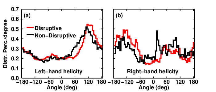
As a rotating mode is slowing down and about to lock, it tends to align with existing = 1 fields. In most cases, this will be the residual error field, defined as the vector sum of the intrinsic error field and the applied = 1 error field correction. Figure 8 shows a histogram of all locked mode phase data, normalized by mode duration and total number of modes in the given set: each mode contributes a total of , where is the total number of disruptive or non-disruptive modes; and further normalized by the binsize of 5 degrees. A clear distribution is observed in figure 8a (left-hand helicity discharges), with a peak at for disruptive modes and for non-disruptive modes. Figure 8b shows right-hand helicity discharges. The disruptive distribution shows an component, though an component is also clearly visible. The non-disruptive distribution shows a strong component. The presence of might be due to occurrences of both over and under correction of the intrinsic error field. Alternatively, the distribution might arise from the presence of both locked and quasi-stationary modes. Locked modes are expected to align with the residual, whereas quasi-stationary modes are expected to move quickly past the residual, spending the most time in the anti-aligned phase. Similar analysis on subsets of these data shows consistent results, suggesting that these distributions are not specific to a certain experimental campaign.
The intrinsic error field in DIII-D has been characterized by in vessel apparatuses [42, 43] and the errors attributed to poloidal field coil misalignments and ellipticity, and the toroidal field buswork. It is found that the intrinsic error is well parameterized by the plasma current and the toroidal field ; "standard error field correction" in the DIII-D plasma control system calculates correction fields based on these. The majority of DIII-D plasmas are run with in the counter-clockwise direction and in the clockwise direction when viewed from above, referred to as the "normal" directions. Taking ranges for and expected to encompass the majority of left-hand helicity discharges (i.e. to 1.5 MA and to -2.1 T), the standard error field correction algorithm applies correction fields between and . The preferential locking angles shown in figure 8a might be due to a residual EF, resulting from the vector addition of the intrinsic EF and an imperfect correction field.
Figures 8c-d show how residual fields can arise from changing intrinsic and/or correction fields. Figures 8e-f illustrate how the distributions in 8a-b might look if the residual is reproducible, or not. In the former case, a narrow, peaked distribution is expected, whereas in the latter case, a broad, flat distribution is expected. This might explain the distributions in figures 8a-b. In addition, quasi-stationary modes are also present in these data, and contribute to the broadening.
6.2 Change in field at locking and growth before disruption
Figure 9 shows the change in mode width as the NTM slows from rotating at kHz to 50 ms after locking. To within the cm errors on the width estimate from magnetics, a significant growth or decay at locking is not observed for the majority of modes. Only 10% of locked modes appear above the top diagonal dashed line, indicating a growth at locking beyond error.
It has been observed across the database that the radial field measured by the ESLDs tends to grow before disruption. This growth is distinct from the dynamics of the locking process, as it often occurs hundreds of milliseconds after locking. Figure 10a shows the behavior before disruption for five randomly chosen disruptive IRLMs. A general period of growth occurs between and 5 ms prior to the disruption, followed by a sharp rise in within milliseconds of the current quench, marked by the transient rise in . Although interesting in its own right, we will not investigate the details of the spike occurring near the current quench, as we are interested in the dynamics leading up to the thermal quench.
Histograms in radial field are plotted in figure 10b, at times before disruption, to study the average evolution. The field in a single case often follows a complicated trajectory, as evidenced by figure 10a, but these histograms reveal global trends. In Figure 10b, the centers of the distributions shift to higher values of as the disruption is approached. The median is chosen to be the representative point in the analysis that follows. The median is the point on the distribution which divides the area under the curve equally.
The median is plotted in figure 10c as a function of time (note the vertical axis is logarithmic). The median major radial field is about 7 G at saturation (i.e. 50 ms after locking). Later in the lifetime of the mode, and approximately 50 ms prior to the disruption, the median grows consistent with an exponential from the saturated value, reaching a final value of G at ms before the disruption. This time is approximately coincident with the onset of the thermal quench. From the slope of the dashed line, in figure 10c, an exponential -folding time for in the range ms is found.
The present analysis is not sufficient to discern between possible sources of this increased . Out of the 26 IRLMs for which 2/1 modes can be clearly seen on ECE (see discussion in section 2.4), less than 10 of these provide a view of the island O-point during the disruption. One such case is shot 157247 shown in figure 11 which disrupted at ms. A significant flattening of the profile is seen at each time slice, confirming that a 2/1 island with cm is present. The solid horizontal bars show the calculated island position (from EFIT) and width (derived from , see Appendix B). The solid line in figure 11b shows the toroidal location of the island O-point on the outboard side in the midplane, and it is seen to intersect the location of the ECE diagnostic (dashed horizontal) at ms. The vertical dashed lines show the times of the profiles in figure 11a. Note that the worst toroidal alignment for O-point viewing occurs for , where the X-point is aligned with the ECE. The horizontal bar at 3710 ms (green in online version) looks to over predict the island width by cm, though the island toroidal alignment with the ECE is intermediate between the O and X-points, where the flattened region is expected to be smaller. EFIT data do not exist for the last two timeslices.
In all shots where magnetics predict O-point alignment with ECE during the disruption, a clear flattening of the profile like that shown in figure 11 is observed. We conclude that the assumption of the presence of an island during the disruption is accurate, and in the shots where ECE data are available, the predicted island widths are reasonable.

If we assume that the increase in the field measured by the ESLDs is due to growth of the 2/1 island, we can estimate how much the island width would increase. We assume a constant , , and during the ms of growth, where the field increases from 7 to 11 G. Therefore, from equation 17, we expect the island width to increase by . With an average saturated width for disruptive islands of cm (this will be shown in section 8), a disruptive island would be expected to grow cm during the exponential growth. With a channel spacing of 1-2 cm for ECE measurements, and with less than 10 disruptive IRLMs whose O-points are well aligned with the ECE diagnostic during this time interval, validating this small change in island width would be difficult.
As the poloidal harmonic of this exponentially growing field is unknown, in principle it is possible that the 2/1 island is unchanging, while an or instability is appearing and growing. Coupling of the 2/1 and 3/1 modes has been observed on ASDEX-Upgrade [44] and investigated in numerical studies [45], while coupling of the 2/1 and has been observed on TEXTOR [46], the RTP Tokamak [14], and studied in simulations [41]. Although might be a candidate for this growth in some shots, it will be shown in section 8 that more than half of the disruptive discharges have , so it could only explain a minority of cases. Similarly, out of 13 IRLMs that occur in plasmas with , at least 7 show a clear disruptive growth, in which the or modes are the only candidates for this growth.
Note that although we have chosen to characterize the final disruptive growth prior to the final thermal quench here, a single mode might undergo multiple growths and minor disruptions, as shown in figure 1.
7 Interdependence of locked modes and
7.1 Effect of locked mode on and equilibrium
A common sign of the existence of a LM is a reduction in plasma . Here we investigate as it has been shown to affect NTM onset thresholds [47] ( is the plasma minor radius and is usually taken to be the toroidal field on axis).
Figure 12a shows at locking as a function of at mode onset. Raw data for disruptive modes are shown in red and purple. The purple disruptive modes are preceded by an earlier LM, while the red are not. The majority of the red points are observed to lie below the dashed diagonal. This observation is reiterated by the light blue points, showing the average and standard deviation also lying predominantly below the diagonal, meaning that decreases from NTM onset to locking.
Notice that a significant population of purple points lie above the dashed line for at rotating onset < 1.5. The rotating phase of these IRLMs begins with frequency (locked), at which point they spin up. In these cases, has suffered a large degradation from the previous locked mode. In most of these cases, the at the following locking is greater than the degraded at the time of spin up, and therefore the points lie above the dashed line.

The light blue and black averages from figure 12a are replotted in figures 12b and 12c in the form of percent changes in at each stage, relative to the at rotating onset. These plots show how changes from the rotating onset to locking, to saturation, and to mode termination. The time of saturation is taken to be 200 ms after locking (found empirically, in approximate agreement with twice the typical DIII-D energy confinement time, ms), and the time of mode termination is taken to be 50 ms before disruption or disappearance of the mode. Except for the initial phase with at rotating onset < 1.5, a continuous decrease in is observed during successive phases of the IRLM.
On average, the disruptive modes cause a larger degradation of than non-disruptive modes during all three phases. For at rotating onset > 1.6, disruptive modes cause 20-50% reduction during the rotating phase, 50-70% reduction by saturation, and 50-80% reduction within 50 ms of the disruption. Of course a further, complete loss of occurs at disruption (not shown).
With the reduction in in figure 12, and assuming constant and (which is accurate for most modes occurring during the flattop), a similar reduction in is expected as well. The reduction in causes a reduction in the Shafranov shift. Figure 13 shows the linear dependence of on during the first 200 ms after locking. A linear fit to the disruptive data provides a shift ratio of cm. Most modes reduce the Shafranov shift by 0-3 cm. This reduction of the shaping reduces toroidal coupling of the and modes, the and modes, and other and mode combinations [48]. The larger scatter in the non-disruptive population can be explained at least in part by significant shape changes, such as the transition from diverted to wall limited. For this reason, the linear fit is performed only on the disruptive data.

7.2 Effect of on the saturated width, IRLM rate of occurrence, and disruptivity
As NTMs are the result of helical perturbations to the bootstrap current [10], we expect the island width to depend on terms that drive the bootstrap current. The Modified Rutherford Equation (MRE) has been shown in previous works to describe 3/2 [6, 49] as well as 2/1 [50, 51] tearing mode saturation well. The saturated modes of interest here have an average width cm and a standard deviation cm. Being that small island terms in the MRE start to become small for cm (assuming cm [10]), small island effects are ignored. A steady state expression of the MRE (i.e. ) is given as follows,
| (2) |
where is the classical stability index, is an ad hoc accounting for the stabilizing effect of field curvature ( for typical DIII-D parameters), is the local inverse aspect ratio, is the length scale of the safety factor profile, is the length scale of the electron pressure profile ( as defined), is the electron poloidal beta, and is the vacuum island width driven by the error field ( cm in DIII-D). Note that usually a cosine term appears on the term involving [52], but it is set to unity here, which assumes the most destabilizing alignment of the locked mode with the error field.
We take to be of the form [8]. With this definition of , equation 2 is a nontrivial cubic equation in . However, an approximate solution was found by approximating (with , , found to be accurate to within 15% over the domain ). The resulting equation is quadratic, of straightforward solution. The approximate saturated width expression is given by,
| (3) |
The data in figure 14 show the normalized island width as a function of . The parameters and are difficult to acquire with automated analysis, and therefore are not available in the database. Therefore, a direct fitting of equation 3 is not appropriate, but the conclusion that increases with is evident. A correlation of is found between and for plasmas with . Plasmas with show a weaker correlation with . This correlation suggests that locked modes in DIII-D are driven at least in part by the bootstrap current.
A one dimensional study of IRLM frequency (or prevalence) versus appears to suggest that intermediate shots are the most prone to IRLMs, as shown in figure 15. The fraction of shots containing an IRLM increases with up to 2.75.
The fraction of shots with IRLMs decreases significantly for . A manual investigation of the 38 shots in the bin reveals that these discharges often have (1) , or (2) high neutral beam torques of Nm, or both. In both cases, a low occurrence of IRLMs might be expected due to a weak wall torque (see equation 1): (1) the surface is far from the wall in discharges with high , and (2) shots with high injected torque likely exhibit high plasma rotation, where the wall torque goes like , and is therefore relatively small. A three-dimensional analysis of IRLM frequency versus , , and NBI torque might be more informative. These data are not populated for all shots in the database, so this analysis is reserved for future work.


The IRLM shot disruptivity as a function of and is plotted in figure 16. The IRLM shot disruptivity is defined as the "number of shots with disruptive IRLMs" divided by the "number of shots with IRLMs". Considering IRLM shot disruptivity as a function of only, the histogram at the right of figure 16a shows a peaked distribution, with the highest values for . Similar results were obtained for the global disruptivity as a function of at NSTX [17] (the NSTX study is not limited to locked modes, and disruptivity is normalized by the amount of time spent at the given value). Reduced locked mode disruptivity at high was also observed at MAST [30].
The IRLM shot disruptivity dependence on can be explained in part by the reduced number of discharges with when is high. To see this, we bin the data in figure 16a into five windows, denoted , , . First, note that figure 16b shows a general decrease in IRLM disruptivity as is increased, across all windows. Next, figure 16c shows the percent distribution of values in each of these windows. The two highest values of (purple and green) have the lowest percentage of discharges with , and the highest percentage of discharges with between 4.5 and 5. This distribution of reduces the number of disruptive discharges, with the net result that the higher discharges appear less disruptive.
As is shown here to affect IRLM shot disruptivity, fixing removes one variable, and allows us to more closely inspect the dependence of IRLM shot disruptivity on . Figure 16b shows IRLM shot disruptivity across five windows in (denoted by color), for five values of (separated by vertical gray lines). In all windows, there is either no significant dependence on , or a lower IRLM shot disruptivity at higher , particularly in the window . Although larger islands are expected at higher , it will be shown in the next section that IRLM disruptivity depends very weakly on island width (refer to figure 18), which in turn might explain the weak dependence on . It should be noted that only is fixed here. Other parameters that are correlated with (e.g. NBI torque, ion and electron temperatures, and possibly others) are not fixed, and might affect the apparent IRLM disruptivity scaling.
8 IRLM disruptivity
8.1 Decoupling the effects of , , and on IRLM disruptivity
Figure 17a shows the normalized radius of the surface and at the mode end, defined here to be 100 ms prior to the termination of the mode. The data are from equilibrium reconstructions constrained by both the external magnetics, and the Motional Stark Effect (MSE) diagnostic. On the right and below figure 17a are histograms of IRLM disruptivity as a function of and respectively. The histogram shows the expected result that lower is more disruptive, as was also seen in figure 16b. The total disruptivity (i.e. not limited to IRLM disruptions) is observed to increase as is decreased in DIII-D [20]. This is in agreement with, but not limited to, observations from JET [15], NSTX [17], and MAST [30]. The histogram in has a qualitatively similar shape, with the highest IRLM disruptivity at large , and the lowest at small .
The raw data show an expected correlation between and . In a circular cross-section, cylindrical plasma, can be defined as follows,
| (4) |
where is the total toroidal current enclosed by the surface, and is the total toroidal current outside of the surface. Note that the quotient behaves similar to the inverse plasma internal inductance : when is large, is small, and vice versa. The lack of one-to-one relationship between and in the raw data of figure 17a may therefore be attributed in part to variations in . Toroidal geometry and plasma shaping may also introduce variations in the relationship between and .
Empirically, we find a high correlation () between and , suggesting a relationship of the form,
| (5) |
where , and . This equation suggests that specifies , or vice versa. We begin by studying the effects of , , and on IRLM disruptivity individually. Then, we investigate IRLM disruptivity as a function of and , which despite the high correlation between the two, reveals that distinguishes disruptive IRLMs better than .
First, to decouple the effect of and on IRLM disruptivity, we fix one and study the dependence on the other in figure 17. We approximately fix by considering only data that lie in small windows of denoted , , , and ( covers a relatively large window in as data become sparse, but IRLM disruptivity appears constant throughout the window). IRLM disruptivity as a function of in the windows is shown in figure 17b. Neither the trace corresponding to nor show a significant trend with IRLM disruptivity beyond error. Both and show a possible decrease in IRLM disruptivity for , but appear constant for .
The same study is performed on by choosing windows in (or safety factor) denoted SF1, SF2, and SF3 (figure 17c). The three safety factor windows agree within statistical error on an increasing linear trend, with IRLM disruptivity for , and for .
From equation 5, we see that fixing and varying (as in figure 17b) implies a variation of as well. The weak or absent trend in IRLM disruptivity as a function of might be explained by competing effects of and .
Similarly, equation 5 shows that fixing and varying (as in figure 17c) also implies varying . The strong dependence of IRLM disruptivity on thus suggests that either , , or both have a strong effect on IRLM disruptivity.

To help isolate the individual effects of , , and , we compare how well they separate disruptive and non-disruptive IRLMs single-handedly.
In order to quantify separation of the distributions in one-dimension, we employ the Bhattacharyya Coefficient (BC) [53]. This coefficient was developed to measure the amount of overlap between two statistical distributions, and is commonly used in image processing, particularly for measuring overlap of color histograms for pattern recognition and target tracking [54]. For two discrete probability distributions and parameterized by , the Bhattacharyya Coefficient is given by,
| (6) |
The metric varies over the range , where a value of 1 indicates that and are identical and perfectly overlapping. A value of 0 implies they are completely distinct (no overlap)
Figure 18 shows the 1D separation of disruptive and non-disruptive modes for six parameters at 100 ms before mode termination, and reports the value for each. Of the three interdependent parameters (i.e. , , and ), is observed both visually, and by the value to best separate the two populations. The parameters and produce less separation with coefficients of and respectively. All BC values reported in figure 18 have an error bar of .

Disruptivity is found to scale strongly with plasma shaping in NSTX [17]. The effects of shaping on IRLM disruptivity in DIII-D will be included in a future work.
8.2 Decoupling effects of and on IRLM disruptivity
In the previous section, it is assumed that and are effectively equivalent, as suggested by equation 5. However, here we show that has a stronger effect on IRLM disruptivity. Figure 19 shows all disruptive and non-disruptive IRLMs plotted in the 2D space of and at 100 ms prior to mode termination.
The data in the region where show a clear vertical separation, rather than a horizontal one. For instance, choosing a threshold of as the definition of a non-disruptive IRLM results in 7% mis-categorized disruptive IRLMs, and 24% mis-categorized non-disruptive IRLMs. To capture a similar number of correctly identified non-disruptive IRLMs using , a value of is used and results in 14% mis-categorized disruptive IRLMs, and 25% mis-categorized non-disruptive IRLMs. This confirms the result of figures 18b-c that categorizes disruptive and non-disruptive IRLMs better than .
To reduce mis-categorized disruptive modes, a threshold of can be used which produces only 3% mis-categorized disruptive IRLMs. However, the mis-categorized non-disruptive IRLMs increase to 42%.
8.3 discriminates disruptive IRLMs within 20 ms of disruption
In this subsection and subsection 8.4, it is assumed that the exponential growth in (figure 10c) is due to growth of the 2/1 island. It will be shown here that is as effective as at discriminating disruptive IRLMs within 20 ms of the disruption. A possible physical interpretation will be given in section 9.
Figure 20 shows the island half-width as a function of the distance between the surface and the unperturbed plasma separatrix, . The shortest perpendicular distance from the black dashed line representing the unperturbed last closed flux surface (LCFS) to a given point is what we have called . In other words, a point appearing near the solid black line represents an island whose radial extent reaches near the unperturbed LCFS. Due to the perturbing field of the locked mode, we expect kinking of the LCFS. This kinking of the LCFS is not accounted for in our calculation of .
is shown to separate disruptive and non-disruptive modes as effectively as at 100 ms prior to disruption in figure 18 (recall the error bar on all BC values). Within 20 ms of the disruption, separates the two populations better with a BC value of 0.61 (compare the dotted red and solid black distributions for in figure 18a). The better separation is due to the exponential growth of the field that occurs in the final 50 ms before disruption: that growth of , and thus of , decreases without affecting . Note that evaluating at 20 ms prior to the disruption implicitly attributes the exponential growth to a growing 2/1 island, but the validity of this assumption does not affect the discrimination ability of .
Choosing a threshold of cm evaluated 20 ms before the disruption (blue dashed line in figure 20), we find 8% mis-categorized disruptive IRLMs, and 28% mis-categorized non-disruptive IRLMs. This is comparable with the 7% and 24% found for , though is evaluated 80 ms earlier (these thresholds on and correctly categorize 195 and 194 non-disruptive IRLMs respectively). A more conservative threshold of cm produces 3% mis-categorized disruptive IRLMs, and 58% mis-categorized non-disruptive IRLMs.
8.4 Weak dependence of IRLM disruptivity on island width
The island width alone is found to be a poor discriminator of disruptive IRLMs at times 20 ms before the disruption or earlier (figure 18f). From the time of saturation until ms prior to the disruption, disruptive and non-disruptive island widths are similar, with a slight tendency for non-disruptive modes to be larger at the earlier times. IRLM disruptivity as a function of the island half-width is shown in the histogram on the right of figure 20. For the majority of islands with half-widths between 2 and 5 cm, IRLM disruptivity does not change significantly, and might be constant within statistical error.
The region below the curved dashed line in figure 20 shows the approximate mode detection limit due to typical signal-to-noise-ratio discussed in section 2.4. Modes appearing in this region were once above the detection limit, and are still measured due to the asymmetry in onset and disappearance thresholds used in the analysis. It is possible that undetected modes in this region might affect the resulting IRLM disruptivity.

8.5 IRLM disruption prediction
Thus far we have discussed percent mis-categorizations, separation of disruptive and non-disruptive distributions measured by the BC coefficient, and IRLM disruptivity all at specific points in time. Although useful for understanding the physics of IRLM disruptions, single time-slice analysis is not sufficient for disruption prediction. Prediction during the locked phase requires establishing a parameter threshold that will never be exceeded by a non-disruptive IRLM, but will be exceeded by a disruptive IRLM at some point before the current quench.
We consider and separately as IRLM disruption predictors. These predictors are intended to be used only in the presence of a detected locked mode. Table 2 shows the percent missed disruptions and percent false alarms for the given thresholds, and for the given warning times. The percent missed disruptions is defined as the number of disruptive IRLMs that do not exceed the threshold within ms of the disruption, divided by the total number of disruptive IRLMs. The percent false alarms is defined as the number of shots where at least one non-disruptive IRLM exceeds the threshold at any time during its lifetime, divided by all issued alarms. Note that a single non-disruptive discharge can have multiple non-disruptive IRLMs, but only one alarm.
If all IRLMs are considered disruptive, no IRLM disruptions are missed, but the percent false alarms increases to . This case is shown as the third row of table 2, labeled “none”, as no additional condition is required before issuing an alarm. Declaring an IRLM disruptive when it locks provides a warning time that depends on the survival time of the IRLM. The distribution of survival times, and therefore also of warning times for this disruption prediction criterion, are shown in figure 6.
| Condition | (%) Missed | (%) False | ||
|---|---|---|---|---|
| with IRLM | disruptions | alarms | ||
| with warning | with warning | |||
| 100ms | 20ms | 100ms | 20ms | |
| cm | ||||
| None | 0 | |||
Despite the seemingly short warning timescale, 20 ms is a sufficient amount of time to deploy massive gas injection in DIII-D [56].
Out of the 53 disruptive discharges omitted due to insufficient equilibrium data (see section 2.4), 17 of them might contribute to increasing the missed disruption percentages associated with the criterion reported in table 2 by up to , with negligible effect on the percent false alarms. Also, out of the remaining disruptive discharges that satisfy , 32 exhibit survival times around 20 ms, and thus the warning time for these modes is no longer than 20 ms. The increase in missed disruptions can be reduced to 1.5% by considering discharges with only, as 9 of the 17 discharges contributing to the increased percent missed disruptions satisfy this criterion (only 40 discharges with 2/1 IRLMs in the entire database satisfy this criterion). The effects of these omitted discharges on the prediction criterion are expected to be similar to those just discussed for the prediction criterion.
8.6 evolution
The evolution of between locking and mode end, provides insight into the evolution of both and . Figure 21a shows that tends to increase by between locking and mode end. This is noticeable by the clustering of points above the dashed diagonal. Equation 5 suggests that an increase in at fixed implies an increase in . As , , and plasma shaping are fixed via feedback in most DIII-D discharges, the assumption of constant is very reasonable. The increase in during locked modes agrees with earlier works [12, 13, 14].

9 Discussion
The physical significance of might be related to the potential energy available for tearing growth (i.e. to the island width dependent classical stability index ).
A one-dimensional simulation including both MHD evolution and transport has shown that the constraint enforced by the sawtooth instability has a significant effect on the current profile, resulting in a steepening of the current gradient between the and surfaces as the edge value is decreased [57]. A steepened current profile on the core-side of the 2/1 island is classically destabilizing, and thus, is shown to increase as the edge decreases.
A three-dimensional simulation [58] later corroborated the classically destabilizing phenomenon found in [57]. Citing these works, a study followed [55], where stability was investigated as a function of the current profile shape, with fixed axial and edge values. In that study, monotonically decreasing current profiles with were varied in search of a stable profile, and a limit in and space was found where no stable solution exists (see figure 6 of [55]). That limit is similar to the empirical IRLM disruption limit shown by the cyan dashed line in figure 22. These three works together [57, 58, 55] provide a theoretical basis for the hypothetical connection between and .
might be responsible for the pre-thermal quench growth shown in figure 10, and it might also influence the evolution of MHD during and after the thermal quench.
Separately, it is interesting that at high density, a high value of is itself unstable, causing radiative contraction of the temperature and current profiles [13], which further increases . Since is approximately fixed via feedback, increasing implies increasing .
Alternatively, the physical significance of might be related to an excess of radiative losses in the island, overcoming the Ohmic heating, resulting in exponential growth [59]. Figure 22 shows good separation of disruptive and non-disruptive IRLMs in the and space used in reference [13] to identify density limit disruptions. Although the plasmas discussed herein are expected to be far from the density limit [60] as a result of the degraded confinement, they are likely near the radiative tearing instability limit which is theorized as the fundamental mechanism causing the density limit [61]. This radiative tearing instability limit is expected qualitatively to scale with .
and are both good IRLM disruption predictors and are both correlated with (the former by equation 5, and the latter by definition). Although this does imply some common underlying physics, and differ from by capturing information on the -profile shape and the island width respectively. Both discriminate disruptive from non-disruptive IRLMs better than alone, and do so by leveraging different physics. We conjecture that is a proxy for , as discussed earlier in this section and supported by earlier publications. The success of the parameter might suggest a position-dependent critical 2/1 island width, where criticality depends on proximity to the unperturbed last closed flux surface. Alternatively, if the field is the result of multiple islands and not just the 2/1 island, as implicitly assumed in the definition of , then island overlap might result from islands of becoming closer and larger as decreases. Island overlap is known to cause stochastic fields [62], and their effect on confinement might be sufficient to induce a disruption. Commonalities and differences between and will be the subject of future work.
Other works have found parameters similar to to be relevant to the onset of the thermal quench, and are briefly listed here. In reference [40], a stable Alcator C-Mod equilibrium is used as an initial condition for a numerical simulation of massive gas injection. It is found that by uniformly distributing a high-Z gas in the edge, a 2/1 island is driven unstable and upon intersecting with the high-Z gas (i.e. when becomes small), the 2/1 grows rapidly followed by a 1/1 tearing mode that leads to a complete thermal quench. Similarly, a limited plasma is simulated in reference [41] with a current profile unstable to the 2/1 island, and the plasma current is ramped up to drive the 2/1 island towards the plasma edge. It is found that when the 2/1 island comes into contact with the limiter or a cold edge region (i.e. in both cases, when is small), a rapid growth of the 2/1 ensues followed by a 1/1 kink displacement of the core, ending in a disruption. Similarly, experimental results of disruptions induced by EF penetration modes on COMPASS-C [39] are attributed to exceeding a threshold of , where and are the 2/1 island width and minor radius. This observation is thought to be due to the 2/1 island interacting with a 3/1 island.
Large 3-D fields at the plasma separatrix cause radial deformations of the edge plasma, leading to edge flux-surfaces (like the when is small) intersecting the vessel [63]. Further, some works suggest the existence of a stochastic layer within the LCFS [64, 65], which might facilitate stochastization of the island when is sufficiently small.
Separately, the radiation drive of tearing modes is sensitive to edge proximity [59], causing island growth which reduces , and could then lead to the thermal quench through one of the above mechanisms. Again, recall that our interpretation of at 20 ms prior to the disruption requires the exponential growth observed in the signal to be due to the 2/1 island growth, which is plausible but not confirmed due to lack of poloidal harmonic analysis in the locked phase. Regardless of the theoretical interpretation, is a useful IRLM disruption predictor within 20 ms of the disruption for DIII-D.
Summary and conclusions
Approximately 22,500 DIII-D plasma discharges were automatically analyzed for the existence of initially rotating 2/1 locked modes (IRLMs). The results of this analysis permits statistical analysis of timescales, mode amplitude dynamics, effects of plasma and major radius , and disruptivity as a function of plasma and mode properties.
Timescales investigated suggest that a rotating 2/1 NTM that will eventually lock rotates for ms, decelerates from kHz to locked in ms, and survives as a locked mode for ms (these values all represent the most frequent value in their respective histograms). These timescales provide insight into how to respond to a mode locking event, whether with a disruption avoidance approach (such as fast controlled shut-down, mode spin-up, or mode stabilization) or a disruption mitigation system (such as massive gas injection), depending on the response times of different systems and approaches.
Prior to disruption, the median perturbed field grows consistent with exponential with an -folding time between ms, which might be due to exponential growth of the 2/1 IRLM.
The parameter is shown to have a strong ability to discriminate between disruptive and non-disruptive IRLMs, up to hundreds of milliseconds before the disruption. As an example, the criterion in the presence of a detected IRLM misses only 7% of disruptions and produces 11% false alarms, with at least 100 ms of warning time. might be related to the free energy available to drive tearing growth.
performs comparably to in its ability to discriminate disruptive IRLMs. A threshold below which IRLMs are considered disruptive of cm produces 4% missed disruptions and 12% false alarms, with at least 20 ms of warning time. is also observed to exhibit the best correlation with the IRLM survival time. might be a fundamental trigger of the thermal quench, supported by similar observations by other authors [39, 41, 40, 63].
Future work will attempt to validate thermal quench onset mechanisms in plasmas with locked modes, with the goal of a fundamental understanding of locked mode disruptions, and thus how to avoid them.
10 Acknowledgements
This work was conducted in part under the DOE Grant DE-SC0008520. In addition, this work is supported by the U.S. Department of Energy, Office of Science, Office of Fusion Energy Sciences, using the DIII-D National Fusion Facility, a DOE Office of Science user facility under awards, DE-FG02-04ER547611, DE-FC02-04ER546982, and DE-FG02-92ER541393. DIII-D data shown in this paper can be obtained in digital format by following the links at https:fusion.gat.comglobal.D3D_DMP.
The authors would like to thank E.J. Strait and R.J. Buttery for carefully reading the manuscript, and A. Cole, J. Hanson, E. Kolemen, M. Lanctot, L. Lao, C. Paz-Soldan, D. Shiraki, and R. Wilcox for fruitful conversations that contributed to this work. The authors would also like to thank S. Flanagan and D. Miller for their computer expertise in developing this database, and M. Brookman for assistance in preparing the electron cyclotron emission data.
References
References
- [1] T.C. Hender, J.C. Wesley, et al. Nucl. Fusion, 47:S128–S202, 2007.
- [2] R.J. La Haye et al. Phys. Plasmas, 10(9), 2003.
- [3] J.A. Snipes et al. Nucl. Fusion, 28(6), 1988.
- [4] R. Fitzpatrick. Nucl. Fusion, 33(7), 1993.
- [5] J.L. Luxon. Nucl. Fusion, 42:614–633, 2002.
- [6] R.J. Buttery et al. Plasma Phys. Contr. Fusion, 42:B61–B73, 2000.
- [7] P.H. Rutherford. Phys. Fluids, 16(11), 1973.
- [8] R.B. White, D.A. Monticello, and M.N. Rosenbluth. Phys. Rev. Lett., 39(25), 1977.
- [9] Z. Chang, J.D. Callen, E.D. Fredrickson, et al. Phys. Rev. Lett., 74(23), 1995.
- [10] R.J. La Haye. Phys. Plasmas, 13(055501), 2006.
- [11] Z. Chang and J.D. Callen. Nucl. Fusion, 30(2), 1990.
- [12] J.T. Scoville, R.J. La Haye, et al. Nucl. Fusion, 31(5), 1991.
- [13] J.A. Wesson, R.D. Gill, M. Hugon, F.C. Schüller, J.A. Snipes, D.J. Ward, et al. Nucl. Fusion, 29(4), 1989.
- [14] F.C. Schüller. Plasma Phys. Contr. Fusion, 37:A135–A162, 1995.
- [15] P.C. de Vries, M.F. Johnson, I. Segui, et al. Nucl. Fusion, 49(055011), 2009.
- [16] P.C. de Vries and M.F. Johnson. Nucl. Fusion, 51(053018), 2011.
- [17] S.P. Gerhardt et al. Nucl. Fusion, 53(043020), 2013.
- [18] S.P. Gerhardt, D.S. Darrow, et al. Nucl. Fusion, 53(063021), 2013.
- [19] R. Yoshino et al. J. Plasma Fusion Res., 70:1081–1101, 1994.
- [20] A.M. Garofalo et al. Fusion Eng. Des., 89:876–881, 2014.
- [21] B. Cannas, A. Fanni, G. Pautasso, G. Sias, et al. Fusion Eng. Des., 86:1039–1044, 2011.
- [22] G. Pautasso, C. Tichmann, S. Egorov, T. Zehetbauer, et al. Nucl. Fusion, 42:100–108, 2002.
- [23] G.A. Rattá, J. Vega, A. Murari, G. Vagliasindi, M.F. Johnson, P.C. de Vries, et al. Nucl. Fusion, 50(025005), 2010.
- [24] R. Yoshino. Nucl. Fusion, 43:1771–1786, 2003.
- [25] C.G. Windsor, G. Pautasso, C. Tichmann, R.J. Buttery, T.C. Hender, et al. Nucl. Fusion, 45:337–350, 2005.
- [26] J.V. Hernandez, A. Vannucci, T. Tajima, Z. Lin, W. Horton, and S.C. McCool. Nucl. Fusion, 36(8), 1996.
- [27] A. Sengupta and P. Ranjan. Nucl. Fusion, 40(12), 1993.
- [28] D. Wróblewski and G.L. Jahns. Nucl. Fusion, 37(6), 1997.
- [29] Y. Zhang, G. Pautasso, et al. Nucl. Fusion, 51(063039), 2011.
- [30] R.J. Buttery et al. Nucl. Fusion, 44:1027–1035, 2004.
- [31] P.C. de Vries, G. Pautasso, E. Nardon, et al. Nucl. Fusion, 56(026007), 2016.
- [32] K.E.J. Olofsson, J.M. Hanson, D. Shiraki, F.A. Volpe, et al. Plasma Phys. Contr. Fusion, 56(095012), 2014.
- [33] E.J. Strait. Rev. Sci. Instrum., 77(023502), 2006.
- [34] J.D. King, E.J. Strait, R.L. Boivin, D. Taussig, M.G. Watkins, et al. Rev. Sci. Instrum., 85(083503), 2014.
- [35] M.E. Austin and J. Lohr. Rev. Sci. Instrum., 74(3), 2003.
- [36] D. Shiraki, R.J. La Haye, N.C. Logan, E.J. Strait, and F.A. Volpe. Nucl. Fusion, 54(033006), 2014.
- [37] L.L. Lao, H. St. John, and R.D. Stambaugh. Nucl. Fusion, 25(10):1421–1436, 1985.
- [38] B.W. Rice, D.G. Nilson, and D. Wróblewski. Rev. Sci. Instrum., 66(1):373–375, 1995.
- [39] T.C. Hender, R. Fitzpatrick, A.W. Morris, et al. Nucl. Fusion, 32(12), 1992.
- [40] V.A. Izzo. Nucl. Fusion, 46:541–547, 2006.
- [41] A. Sykes and J.A. Wesson. Phys. Rev. Lett., 44(18), 1980.
- [42] R.J. La Haye and J.T. Scoville. Rev. Sci. Instrum., 62:2146–2153, 1991.
- [43] J.L. Luxon, M.J. Schaffer, et al. Nucl. Fusion, 43:1813–1828, 2003.
- [44] H. Zohm, M. Maraschek, G. Pautasso, M. Schittenhelm, S. Sesnic, M. Sokoll, and W. Suttrop. Plasma Phys. Contr. Fusion, 37:A313–A324, 1995.
- [45] V. Igochine, O. Dumbrajs, D. Constantinescu, H. Zohm, G. Zvejnieks, et al. Nucl. Fusion, 46:741–751, 2006.
- [46] P.C. de Vries, G. Waidmann, A.J.H. Donné, and F.C. Schüller. Plasma Phys. Contr. Fusion, 38:467–476, 1996.
- [47] R.J. Buttery, R.J. La Haye, et al. Phys. Plasmas, 15(056115), 2008.
- [48] R. Fitzpatrick. Phys. Plasmas, 1(10):3308–36, 1994.
- [49] R.J. La Haye and O. Sauter. Nucl. Fusion, 38(7), 1998.
- [50] L. Urso, H. Zohm, et al. Nucl. Fusion, 50(025010), 2010.
- [51] Kyungjin Kim, Yong-Su Na, Minhwa Kim, et al. Curr. Appl. Phys., 15:547–554, 2015.
- [52] R. Fitzpatrick. Phys. Plasmas, 5(9), 1998.
- [53] A. Bhattacharyya. Indian J. Statistics, 7(4), 1946.
- [54] D. Comaniciu and V. Ramesh. Comput. Vision Pattern Recog., 2:142–149, 2000.
- [55] C.Z. Cheng, H.P. Furth, and A.H. Boozer. Plasma Phys. Contr. Fusion, 29(3):351–366, 1987.
- [56] N.W. Eidietis et al. Nucl. Fusion, 55(063030), 2015.
- [57] M.F. Turner and J.A. Wesson. Nucl. Fusion, 22(8):1069–78, 1982.
- [58] A. Bondeson. Nucl. Fusion, 26(7):929–40, 1986.
- [59] R.B. White, D.A. Gates, and D.P. Brennan. Phys. Plasmas, 22(022514), 2015.
- [60] M. Greenwald, J.L. Terry, and S.M. Wolfe. Nucl. Fusion, 28(12), 1988.
- [61] D.A. Gates and L. Delgado-Aparicio. Phys. Rev. Lett., 108(165004), 2012.
- [62] P.H. Rebut and M. Hugon. IAEA Proceedings, pages 197–211, 1984.
- [63] T.E. Evans, R.K.W. Roeder, J.A. Carter, B.I. Rapoport, M.E. Fenstermacher, and C.J. Lasnier. J. Phys., Conference Series 7:174–190, 2005.
- [64] T.E. Evans, R.A. Moyer, and P. Monat. Phys. Plasmas, 9(12), 2002.
- [65] V.A. Izzo and I. Joseph. Nucl. Fusion, 48(115004), 2008.
- [66] J.A. Wesson, D.J. Campbell, J.W. Connor, R.D. Gill, J. Hugill, C.N. Lashmore-Davies, G.M. McCracken, H.R. Wilson, et al. Tokamaks, page 366. Clarendon Press - Oxford, third edition, 2004.
Appendix A - Mapping from radial field to perturbed island current
A model was produced to map from the value of the major-radial magnetic field at the external saddle loops to the perturbed current carried by a circular cross-section toroidal current sheet. This model was inspired by a similar technique that accurately reproduced experimental magnetic signals in DIII-D [36]. The current sheet has major radius and minor radius , derived from equilibrium reconstructions using magnetics and Motional Stark Effect data. A shaping study was performed to test the impact of ellipticity on the external saddle loop measurement. The impact was found to be relatively small, introducing corrections of less than 5%. Hence, it was concluded that circular cross-sections are sufficient for modeling external saddle loop signals for the sake of the present study.
The modeled current sheet is discretized into helical wire filaments with 2/1 pitch giving a toroidal spacing of degrees. The currents are distributed among the wires to produce a 2/1 current perturbation as shown by the colors in figure 23a (black represents no perturbed current and red represents maximum perturbed current).


The field is calculated by numerically integrating the Biot-Savart Law along each wire. Figure 23b shows the resulting major-radial field as "seen" by the external saddle loops, due to a 2/1 current distribution. The color contour shows a clear field distribution. Although the external saddle loops have complete toroidal coverage, they have only poloidal coverage for the non-elongated, cylindrically approximated plasma.
A single measurement for each saddle loop is estimated by averaging the field at 100 sample points. Care was taken to ensure the area of each sample point is identical, which simplifies the flux calculation. The field samples are averaged, which is identical to calculating the total flux and dividing by saddle loop area :
| (7) |
where is the total area of one saddle loop, is the constant sample area (i.e. ), is the number of sample regions per saddle loop, and is the major-radial field at the sample region.
The above averaging is done for each of the six saddle loops. The simulated signals are then pair-differenced, and a least squares fit is used to extract the amplitude of the component, in the same way that experimental data are analyzed in section 2.4.

The island current, , is defined as the total current deficit, as seen in figure 24b. A second definition of island current is useful for mapping to a cylindrical island width, being half the sinusoidal perturbed current (see figure 24a). and are related by the equation . The current distribution in figure 24b can be seen as the distribution in 24a, plus an axisymmetric current. The non-axisymmetric fields produced by 24a and 24b are identical.
The component in the external saddle loops, , was then studied as a function of and for fixed island current as seen in figure 25. is found to be quadratic in in agreement with the cylindrical approximation. As is increased, the leading order coefficient of the quadratic is seen to increase as well. Defining the leading order coefficient (which note is a function of ), we find the following relationship:
| (8) |
where is in Gauss, is in kA, and are in meters, and has units of G/kA/m2. Evaluating the change in as a function of , the dependence is found to be well approximated by a second order polynomial where G/kA/m4, G/kA/m3, and G/kA/m2.
With equation 8, experimental measurements from the external saddle loops are mapped to by a simple inversion of the equation and with major and minor radii provided by EFIT informed by magnetics and Motional Stark Effect data:
| (9) |
Appendix B - Mapping from perturbed island current to width
Although the perturbed island current is an intrinsic island quantity that accounts for toroidicity, an island width was desirable for some studies. We will use to map to an island width.
We solve for the radial field at the surface by assuming cylindrical geometry, using the ordering , and assuming vacuum solutions for the radial tearing eigenfunctions. The non-axisymmetric field produced by the island is expressed as,
| (10) |
where is the perturbed flux function which is of the form (note that the toroidal wavelength is assumed infinite here). We assume the perturbed current in the island to be a sheet current located at the surface expressed as,
| (11) |
where is constant with units (A/m), represents the Dirac delta function, and the poloidal harmonic is implied. Invoking Ampere’s law where the time derivative of is neglected (the characteristic velocity of the system ), and the equilibrium plasma current is neglected (i.e. searching for vacuum solutions), we find
| (12) |
Solving the cylindrical Laplacian both inside and outside of the surface, requiring the solutions be continuous across , and defining the jump in the radial derivative with the radial integral of , we find
| (13) |
Using equation 10, the field at the surface is then given by
| (14) |
We now want to replace with an expression for . We do so as follows (see figure 24a),
| (15) |
where , and . After substituting equation 11 and evaluating the integral, we find .
Finally, substituting this into equation 14, we have
| (16) |
The cylindrical island width is given by [66],
| (17) |
where is a toroidal correction for island widths measured at the outboard midplane, is the perturbed radial field at the surface, is the local safety factor, is the poloidal harmonic, is the toroidal field at the magnetic axis, and is the radial derivative of the safety factor evaluated at on the outboard midplane (the cylindrical expression for the safety factor was used here). Substituting and , and using the maximum of equation 16 for , we have
| (18) |
This expression for the island width was validated using the electron cyclotron emission diagnostic [35] to observe the size of flattened regions in the temperature profile. Using nine islands, the toroidal correction factor is calibrated to . Using equation 18, we expect a statistical error on island width estimates. This expression for the island width is used for all plots of and .