跳到论文正文
W Papers独立论文阅读器 arXiv:1606.04131 论文正文 计算阅读时间 · 0%
引用这篇论文根据当前论文元数据生成,正式投稿前建议核对。


License: arXiv.org perpetual non-exclusive license
arXiv:1606.04131v3 [hep-ph] 31 Oct 2016

CERN-PH-TH-2016-140

Bounds on supersymmetric effective operators

from heavy diphoton searches

D. M. Ghilenceaa,b{}^{\,a,\,b} and Hyun Min Leec{}^{\,c}

a Theory Division, CERN, 1211 Geneva 23, Switzerland

b Theoretical Physics Department, National Institute of Physics

and Nuclear  Engineering   (IFIN-HH)  Bucharest  077125, Romania

c Department of Physics, Chung-Ang University, 06974 Seoul, Korea.

Abstract

We identify the bounds on supersymmetric effective operators beyond MSSM, from heavy diphoton resonance (XX) negative searches at the LHC, where XX is identified with the neutral CP-even (odd) HH (AA) or both (mass degenerate). While minimal supersymmetric models (MSSM, etc) comply with the data, a leading effective operator of d=6d=6 can contribute significantly to diphoton production σ∼1\sigma\sim 1 fb, well above its MSSM value and in conflict with recent data. Both the b​b¯b\bar{b} and g​ggg production mechanisms of HH and AA can contribute comparably to this. We examine the dependence of the diphoton cross section σ\sigma on the values of mXm_{X}, Λ\Lambda and tan⁡β\tan\beta, under the experimental constraints from the SM-like higgs couplings h​g​ghgg and h​γ​γh\gamma\gamma (due to mixing) and from the b​b¯b\bar{b} and t​t¯t\bar{t} searches. These give Λ\Lambda larger than ∼5\sim 5 TeV for mXm_{X} in the range 0.5−10.5-1 TeV. We show how to generate the d=6d=6 effective operator from microscopic (renormalizable) models. This demands the presence of vector-like states beyond the MSSM spectrum (and eventually but not necessarily a gauge singlet), of mass near Λ\Lambda and thus outside the LHC reach.

1 Motivation

Current searches for new physics at the LHC bring increasingly strong constraints on the parameter space of supersymmetric models. Consider for example a final diphoton state at the LHC. Then at the parton level, the exchange of a state XX of spin JJ, mass mXm_{X} and width ΓX\Gamma_{X} has a cross section

σ⁡(p​p→X→γ​γ)=2​J+1s​mX​[∑pCp​p¯​Γ​(X→p​p¯)]​Γ⁡(X→γ​γ)ΓX\displaystyle\sigma(pp\rightarrow X\rightarrow\gamma\gamma)=\frac{2J+1}{s\,{m_{X}}}\Big[\sum_{p}C_{p\bar{p}}\,\Gamma(X\rightarrow p\bar{p})\Big]\,\frac{\Gamma(X\rightarrow\gamma\gamma)}{\Gamma_{X}} (1)

where the sum is over partons p={g,b,c,s,u,d,γ}p=\{g,b,c,s,u,d,\gamma\}. Cp​p¯C_{p\bar{p}} are partonic integrals coefficients evaluated at mX{m_{X}}. LHC searches for a heavy diphoton resonance (XX) can impact on model building beyond the Standard Model (SM), in particular on supersymmetric models.

Much interest was raised by the initial claim by ATLAS and CMS Collaborations at s=13\sqrt{s}\!=\!13 TeV of a possible diphoton final state of mX=750m_{X}=750 GeV with an excess relative to the SM [1] (also [2, 3]), with σ​(p​p→γ​γ)ATLAS=10±3​fb\sigma(pp\rightarrow\gamma\gamma)_{\textsf{ATLAS}}=10\pm 3\,\textsf{fb} and σ​(p​p→γ​γ)CMS=6±3​fb.\sigma(pp\rightarrow\gamma\gamma)_{\textsf{CMS}}=6\pm 3\,\textsf{fb}. Further, the analysis of additional data invalidated this claim [4]. This is actually welcome for minimal supersymmetric models (MSSM, etc) where it is not possible to have a heavy resonance XX with such significant σ\sigma [5], except if11 1 Many non-supersymmetric explanations were reported for this 750 GeV “resonance”, see [6] for a long list of references. XX was a scalar singlet with couplings to new TeV states that mediate (at loop level) its production by g​ggg fusion and its decay to γ​γ\gamma\gamma [7, 8]. For a non-supersymmetric effective study see [9, 10].. a): one is fine-tuning the parameters [11] with XX the CP even/odd heavy higgs X=HX=H, AA, or b): considers the rather special case of low, TeV-scale supersymmetry breaking with XX a sgoldstino [12], see also [13, 14, 15].

However, we show that effective operators beyond the MSSM (minimal) higgs sector can contribute dramatically to the diphoton production (giving σ∼\sigma\sim few fb) not seen in the data [4]. The resonance XX is the CP-odd/even neutral MSSM higgs AA or HH or both (mass degenerate). This result is due to enhanced couplings of the higgs sector to SM gauge bosons, induced by the following unique, leading operator of dimension d=6d\!=\!6

(1/Λ2)∫d2θ(H1.H2)TrWαWα+h.c.,\displaystyle(1/\Lambda^{2})\int d^{2}\theta\,(H_{1}.H_{2})\,\mbox{Tr}\,W^{\alpha}W_{\alpha}+\rm{h.c.}, (2)

where WαW_{\alpha} is the supersymmetric field strength of the SM sub-groups U(1)Y, SU(2)L, SU(3).

Depending on Λ\Lambda, operator (2) can bring a large correction to the diphoton production in conflict with the latest data, with impact on H,AH,A searches. Motivated by this, we study the constraints on this operator and examine the dependence of the diphoton cross section σ\sigma on the values of mXm_{X}, Λ\Lambda and tan⁡β\tan\beta, while including both the b​b¯b\bar{b} and g​ggg production mechanisms of X=A,HX=A,H. The experimental constraints on the SM-like higgs (hh) couplings h​g​ghgg and h​γ​γh\gamma\gamma and on the b​b¯b\bar{b} (t​t¯t\bar{t}) cross section (that receive corrections from (2)), are also applied, with impact on the allowed mXm_{X}, Λ\Lambda and tan⁡β\tan\beta. For a given σ∼0.1−1\sigma\sim 0.1-1 fb, we illustrate these constraints for mH,Am_{H,A} in the range 0.5−10.5-1 TeV (in particular for the absent “resonance” at 750750 GeV). We then show how operator (2) is generated in a renormalizable model beyond MSSM; an extra d=5d\!=\!5 operator may also be generated (in some cases) and does not directly affect the diphoton production but may improve naturalness [16].

In section 2 we study the new couplings induced in the MSSM higgs sector by the d=6d\!=\!6 effective operator and its effect on the diphoton production. Section 3 shows how these operators are generated in a renormalizable model. Our conclusions are found in Section 4.

2 Effective operators and diphoton resonance

We consider the MSSM model extended by (supersymmetric) effective operators in the higgs sector and study the diphoton production cross section σ\sigma due to a possible resonance XX identified with HH and/or AA. We compute the corrections to the couplings of HH, AA and hh, and the branching ratios of HH, AA. We then illustrate the correlations between the values of Λ\Lambda, mXm_{X}, tan⁡β\tan\beta and σ\sigma, consistent with the constraints from Higgs signals/decays.

2.1 New couplings from effective operators beyond MSSM

From all effective operators of dimensions d=5d=5 and d=6d=6 [16, 17, 18] beyond the MSSM higgs sector, we find only one leading operator that can contribute to a diphoton resonance

ℒj\displaystyle{\cal L}_{j} =\displaystyle= cj2​Λ2​gj2​κj∫d2θ(H2.H1)Tr(WαWα)j+h.c.\displaystyle\frac{c_{j}}{2\Lambda^{2}\,g^{2}_{j}\kappa_{j}}\int d^{2}\theta\,\,(H_{2}.H_{1})\,\,{\rm Tr}\,(W^{\alpha}W_{\alpha})_{j}+\mbox{h.c.} (3)

which has dimension d=6d=6. Here j=1,2,3j=1,2,3 labels the U(1)Y, SU(2)L, SU(3) gauge groups of gauge couplings gjg_{j}, so we actually have three operators, with coefficients22 2 The coefficients cj=𝒪⁡(1)c_{j}={\cal O}(1), j=1,2,3j=1,2,3 enable us later to turn on/off any of operators ℒ1,2,3{\cal L}_{1,2,3}. cj=𝒪⁡(1)c_{j}={\cal O}(1) and Λ\Lambda a free parameter. κj\kappa_{j} is a constant that cancels the trace factor. (Wα)j(W^{\alpha})_{j} is the field strength of a vector superfield VjV_{j}. The relevant part is33 3 Notation used: h1.h2=h10​h20−h1−​h2+h_{1}.h_{2}=h_{1}^{0}h_{2}^{0}-h_{1}^{-}h_{2}^{+}; also Re​h10=H​cos⁡α−h​sin⁡α\text{Re}\ h_{1}^{0}=H\,\cos\alpha-h\,\sin\alpha, Re​h20=H​sin⁡α+h​cos⁡α\text{Re}\ h_{2}^{0}=H\,\sin\alpha+h\,\cos\alpha.

ℒj⊃cjΛ2[(h1.h2)(Fja​μ​νFj​μ​νa+iFj​μ​νaF~ja​μ​ν)+h.c.]\displaystyle{\cal L}_{j}\supset\frac{c_{j}}{\Lambda^{2}}\,\,\Big[\,(h_{1}.h_{2})\,(F_{j}^{a\,\mu\nu}F^{a}_{j\,\mu\nu}+iF^{a}_{j\,\mu\nu}\tilde{F}^{a\,\mu\nu}_{j})+\mbox{h.c.}\Big] (4)

with F~μ​ν=(1/2)​ϵμ​ν​ρ​σ​Fρ​σ\tilde{F}^{\mu\nu}=(1/2)\,\epsilon^{\mu\nu\rho\sigma}\,F_{\rho\sigma}. With real cjc_{j} one has, in a standard notation

ℒ1+ℒ2\displaystyle\!\!{\cal L}_{1}\!+\!{\cal L}_{2}\!\!\! ⊃\displaystyle\supset vΛ2[(cγ​γh+bγ​γH)Fμ​νFμ​ν+(cγ​zh+bγ​zH)Fμ​νZμ​ν\displaystyle\!\!\!\frac{v}{\Lambda^{2}}\Big[(c_{\gamma\gamma}h+b_{\gamma\gamma}H)\,F_{\mu\nu}F^{\mu\nu}+(c_{\gamma z}h+b_{\gamma z}H)\,F_{\mu\nu}Z^{\mu\nu} (5)
+(cz​z​h+bz​z​H)​Zμ​ν​Zμ​ν+(cw​w​h+bw​w​H)​Wμ​ν+​W−μ​ν\displaystyle\hskip 10.00002pt+\,(c_{zz}h+b_{zz}H)\,Z_{\mu\nu}Z^{\mu\nu}+(c_{ww}h+b_{ww}H)\,W^{+}_{\mu\nu}W^{-\mu\nu}
+aγ​γAFμ​νF~μ​ν+az​zAZμ​νZ~μ​ν+aγ​zAFμ​νZ~μ​ν+aw​wAWμ​ν+W~−μ​ν]\displaystyle\hskip 10.00002pt+\,a_{\gamma\gamma}\,AF_{\mu\nu}\tilde{F}^{\mu\nu}+a_{zz}A\,Z_{\mu\nu}\tilde{Z}^{\mu\nu}+a_{\gamma z}A\,F_{\mu\nu}\tilde{Z}^{\mu\nu}+a_{ww}\,A\,W^{+}_{\mu\nu}{\tilde{W}}^{-\mu\nu}\Big]\hskip 10.00002pt

where Fμ​νF_{\mu\nu} is the photon field strength, HH (AA) are the CP-even (odd) neutral higgses and

aγ​γ=−(c1​cw2+c2​sw2),az​z=−(c1​sw2+c2​cw2),aγ​z=−(c2−c1)​s2​w,aw​w=−2​c2\displaystyle a_{\gamma\gamma}=-(c_{1}\,c_{w}^{2}+c_{2}\,s_{w}^{2}),\hskip 10.00002pt\,a_{zz}=-(c_{1}s_{w}^{2}+c_{2}c_{w}^{2}),\,\,\,\,a_{\gamma z}=-(c_{2}-c_{1})s_{2w},\,\,a_{ww}=-2c_{2}\hskip 20.00003pt\,\,\,\,\hskip 10.00002pt
bγ​γ=−aγ​γ​sα​β,bz​z=−az​z​sα​β,bγ​z=−aγ​z​sα​β,bw​w=−aw​w​sα​β\displaystyle b_{\gamma\gamma}=-a_{\gamma\gamma}\,s_{\alpha\beta},\hskip 20.00003pt\hskip 20.00003ptb_{zz}=-a_{zz}\,s_{\alpha\beta},\hskip 20.00003pt\hskip 10.00002pt\,\,\,b_{\gamma z}=-a_{\gamma z}\,s_{\alpha\beta},\hskip 20.00003pt\,\,\,b_{ww}=-a_{ww}\,s_{\alpha\beta}\hskip 20.00003pt
cγ​γ=−aγ​γ​cα​β,cz​z=−az​z​cα​β,cγ​z=−aγ​z​cα​β,cw​w=−aw​w​cα​β\displaystyle c_{\gamma\gamma}=-a_{\gamma\gamma}\,c_{\alpha\beta},\hskip 20.00003pt\hskip 10.00002pt\,c_{zz}=-a_{zz}\,c_{\alpha\beta},\hskip 20.00003pt\hskip 10.00002pt\,\,\,c_{\gamma z}=-a_{\gamma z}\,c_{\alpha\beta},\hskip 20.00003pt\,\,\,c_{ww}=-a_{ww}\,c_{\alpha\beta} (6)

with the notations: cα​β=cos⁡(α+β)c_{\alpha\beta}=\cos(\alpha+\beta), sα​β=sin⁡(α+β)s_{\alpha\beta}=\sin(\alpha+\beta), c2​β=cos⁡(2​β)c_{2\beta}=\cos(2\beta), cw=cos⁡θwc_{w}=\cos\theta_{w}, sw=sin⁡θws_{w}=\sin\theta_{w}, s2​w=sin⁡2​θws_{2w}=\sin 2\theta_{w}. Let us also consider the effect of the gluon operator44 4 If c3c_{3} has an imaginary part, one also has ℒ3⊃v/Λ2​[a~g​g​A0​Tr​G2+b~g​g​H​Tr​G​G~+c~g​g​h​Tr​G2]{\cal L}_{3}\supset v/\Lambda^{2}[\tilde{a}_{gg}A^{0}\,\mbox{Tr}G^{2}+\tilde{b}_{gg}H\,\mbox{Tr}G\tilde{G}+\tilde{c}_{gg}h\,\mbox{Tr}G^{2}] with a~g​g=−Im​[c3]\tilde{a}_{gg}=-\text{Im}\ [c_{3}], b~g​g=−Im​[c3]​sin⁡(α+β)\tilde{b}_{gg}=-\text{Im}\ [c_{3}]\sin(\alpha+\beta), c~g​g=−Im​[c3]​cos⁡(α+β)\tilde{c}_{gg}=-\text{Im}\ [c_{3}]\cos(\alpha+\beta).

ℒ3⊃vΛ2​[cg​g​h​Tr​Gμ​ν​Gμ​ν+bg​g​H​Tr​Gμ​ν​Gμ​ν+ag​g​A​Tr​Gμ​ν​G~μ​ν]\displaystyle{\cal L}_{3}\supset\frac{v}{\Lambda^{2}}\Big[c_{gg}\,h\,{\rm Tr}\,G_{\mu\nu}G^{\mu\nu}+b_{gg}H\,{\rm Tr}\,G_{\mu\nu}G^{\mu\nu}+a_{gg}A\,{\rm Tr}\,G_{\mu\nu}\tilde{G}^{\mu\nu}\Big] (7)

where

ag​g=−c3,bg​g=c3​sα​β,cg​g=c3​cα​β.\displaystyle a_{gg}=-c_{3},\hskip 20.00003ptb_{gg}=c_{3}\,s_{\alpha\beta},\hskip 20.00003pt\hskip 10.00002ptc_{gg}=c_{3}\,c_{\alpha\beta}. (8)

The Lagrangian of the MSSM corrected with ℒ1,2,3{\cal L}_{1,2,3} induces the following couplings

ℒ\displaystyle{\cal L} =\displaystyle= 1v[(c^γ​γh+b^γ​γH)Fμ​νFμ​ν+(c^γ​zh+b^γ​zH)Fμ​νZμ​ν+(c^z​zh+b^z​zH)Zμ​νZμ​ν\displaystyle\frac{1}{v}\,\Big[(\hat{c}_{\gamma\gamma}h+\hat{b}_{\gamma\gamma}H)\,F_{\mu\nu}F^{\mu\nu}+(\hat{c}_{\gamma z}h+\hat{b}_{\gamma z}H)\,F_{\mu\nu}Z^{\mu\nu}+(\hat{c}_{zz}h+\hat{b}_{zz}H)Z_{\mu\nu}Z^{\mu\nu} (9)
+(c^w​w​h+b^w​w​H)​Wμ​ν+​W−μ​ν+a^γ​γ​A​Fμ​ν​F~μ​ν+a^z​z​A​Zμ​ν​Z~μ​ν+a^γ​z​A​Fμ​ν​Z~μ​ν\displaystyle\,\,+\,\,(\hat{c}_{ww}h+\hat{b}_{ww}H)\,W^{+}_{\mu\nu}W^{-\mu\nu}+\,\,\hat{a}_{\gamma\gamma}\,A\,F_{\mu\nu}\tilde{F}^{\mu\nu}+\hat{a}_{zz}A\,Z_{\mu\nu}\tilde{Z}^{\mu\nu}+\,\,\hat{a}_{\gamma z}\,A\,F_{\mu\nu}\tilde{Z}^{\mu\nu}
+a^w​wAW+μ​νW~μ​ν−+(c^g​gh+b^g​gH)TrGμ​νGμ​ν+a^g​gATrGμ​νG~μ​ν].\displaystyle\,\,+\,\hat{a}_{ww}\,A\,\,W^{+\mu\nu}\tilde{W}_{\mu\nu}^{-}+\big(\hat{c}_{gg}\,h+\hat{b}_{gg}H\big)\,\mbox{Tr}\,G_{\mu\nu}G^{\mu\nu}+\hat{a}_{gg}\,A\,\,\mbox{Tr}\,G_{\mu\nu}\tilde{G}^{\mu\nu}\Big].\hskip 20.00003pt

The coefficients a^\hat{a}, b^\hat{b} and c^\hat{c} above are related to their counterparts without a hat:

τ^γ​γ\displaystyle\hat{\tau}_{\gamma\gamma} =\displaystyle= αem8​π​τγ​γl​o​o​p+v2Λ2​τγ​γ,τ^z​z=αem8​π​τz​zl​o​o​p+v2Λ2​τz​z,\displaystyle\frac{\alpha_{\rm em}}{8\pi}\,\,\tau_{\gamma\gamma}^{loop}+\frac{v^{2}}{\Lambda^{2}}\,\tau_{\gamma\gamma},\hskip 20.00003pt\hskip 10.00002pt\hat{\tau}_{zz}=\frac{\alpha_{\rm em}}{8\pi}\,\tau_{zz}^{loop}+\frac{v^{2}}{\Lambda^{2}}\,\tau_{zz},
τ^g​g\displaystyle\hat{\tau}_{gg} =\displaystyle= α312​π​τg​gl​o​o​p+v2Λ2​τg​g,τ^w​w=αem8​π​τw​wl​o​o​p+v2Λ2​τw​w,\displaystyle\frac{\alpha_{3}}{12\pi}\,\,\tau_{gg}^{loop}+\frac{v^{2}}{\Lambda^{2}}\,\tau_{gg},\hskip 20.00003pt\hskip 10.00002pt\hat{\tau}_{ww}=\frac{\alpha_{\rm em}}{8\pi}\,\tau_{ww}^{loop}+\frac{v^{2}}{\Lambda^{2}}\,\tau_{ww},\,\,\,
τ^γ​z\displaystyle\hat{\tau}_{\gamma z} =\displaystyle= αem8​π​sw​τγ​zl​o​o​p+v2Λ2​τγ​z,where​τ=a,b,c.\displaystyle\frac{\alpha_{\rm em}}{8\pi s_{w}}\,\tau_{\gamma z}^{loop}+\frac{v^{2}}{\Lambda^{2}}\,\tau_{\gamma z},\hskip 20.00003pt\hskip 10.00002pt{\rm where}\,\,\,\tau=a,b,c. (10)

The coefficients multiplying v2/Λ2v^{2}/\Lambda^{2} are those of eqs.(6), (8). Further, the coefficients a..l​o​o​pa_{..}^{loop}, b..l​o​o​pb_{..}^{loop}, c..l​o​o​pc_{..}^{loop} are loop-induced, due to the MSSM (in the absence of the effective operators). They bring a very small branching ratio to photons [5] relative to v2/Λ2v^{2}/\Lambda^{2} terms and we present them in Appendix A in the decoupling limit (α→β−π/2\alpha\rightarrow\beta-\pi/2) in which we work in this paper. We show that their corrected version a^\hat{a}, b^\hat{b}, c^\hat{c} of eqs.(9), (10) can bring a heavy diphoton resonance of large σ∼1\sigma\sim 1 fb, in our model defined by MSSM extended by eq.(3), in possible conflict with the latest data.

2.2 Decay branching ratios of AA and HH

Refer to caption
Refer to caption
Refer to caption
Refer to caption
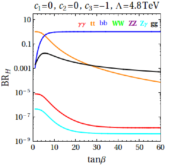
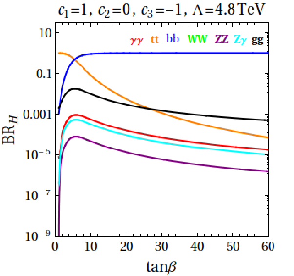
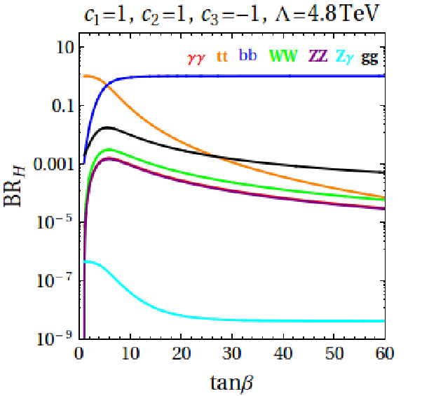
Figure 1: Branching ratios of H→γ​γH\rightarrow\gamma\gamma, t​t¯t\bar{t}, b​b¯b\bar{b}, W​WWW, Z​ZZZ, Z​γZ\gamma and g​ggg, for different c1,2,3c_{1,2,3} and tan⁡β\tan\beta. The case c1=1c_{1}=1, c2=c3=0c_{2}=c_{3}=0 (not shown) is similar to c1=0c_{1}=0, c2=1c_{2}=1, c3=0c_{3}=0 (without W​WWW). The branching ratios for AA into the same final states are similar to those above, for the same parameters. Compared to individual ℒ1,2,3{\cal L}_{1,2,3}, a combination ℒ1+ℒ3{\cal L}_{1}+{\cal L}_{3} or ℒ1+ℒ2+ℒ3{\cal L}_{1}+{\cal L}_{2}+{\cal L}_{3} brings the largest branching ratio of H (A) to γ​γ\gamma\gamma, for appropriate relative signs of cjc_{j}, j=1,2,3j=1,2,3.
Refer to caption
Refer to caption
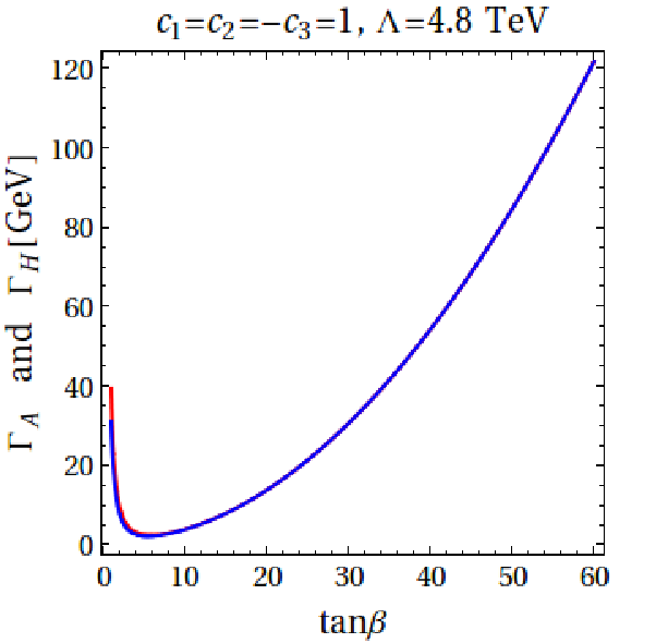
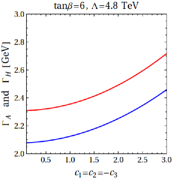
Figure 2: Total decay widths of heavy Higgs fields ΓH\Gamma_{H} (blue) and ΓA\Gamma_{A} (red), for mA,H=750m_{A,H}=750 GeV. These plots remain similar for other c1,c2,c3c_{1},c_{2},c_{3} used later. A narrow width region ΓX≤5\Gamma_{X}\leq 5 GeV corresponds to low ≤tan⁡β≤122\!\leq\!\tan\beta\!\leq\!12 while for larger tan⁡β\tan\beta one has a large width regime.

To discuss the diphoton production we first analyze the impact of the corrections in eq.(9), (10) on the decay rates of the heavy neutral CP-even (odd) Higgs HH (AA), respectively. The decay rate of HH is ΓH=∑iΓ⁡(H→i)\Gamma_{H}=\sum_{i}\Gamma(H\rightarrow i), where

Γ⁡(H→t​t¯)\displaystyle\Gamma(H\rightarrow t{\bar{t}}) =\displaystyle= Nc​mt28​π​v2​cot2⁡β​mH​(1−4​xt)3/2,\displaystyle\frac{N_{c}m^{2}_{t}}{8\pi v^{2}}\,\cot^{2}\beta\,m_{H}(1-4x_{t})^{3/2},
Γ⁡(H→b​b¯)\displaystyle\Gamma(H\rightarrow b{\bar{b}}) =\displaystyle= Nc​mb28​π​v2​tan2⁡β​mH​(1−4​xb)3/2,xi≡mi2/mH2\displaystyle\frac{N_{c}m^{2}_{b}}{8\pi v^{2}}\,\tan^{2}\beta\,m_{H}(1-4x_{b})^{3/2},\hskip 20.00003ptx_{i}\equiv m^{2}_{i}/m^{2}_{H} (11)

valid in the decoupling limit and

Γ⁡(H→γ​γ)\displaystyle\Gamma(H\rightarrow\gamma\gamma) =\displaystyle= 14​π​(b^γ​γv)2​mH3\displaystyle\frac{1}{4\pi}\Big(\frac{\hat{b}_{\gamma\gamma}}{v}\Big)^{2}m_{H}^{3}
Γ⁡(H→γ​Z)\displaystyle\Gamma(H\rightarrow\gamma Z) =\displaystyle= 18​π​(b^γ​zv)2​mH3​(1−xZ)3\displaystyle\frac{1}{8\pi}\Big(\frac{\hat{b}_{\gamma z}}{v}\Big)^{2}m_{H}^{3}\,(1-x_{Z})^{3}
Γ⁡(H→g​g)\displaystyle\Gamma(H\rightarrow gg) =\displaystyle= 2π​(b^g​gv)2​mH3\displaystyle\frac{2}{\pi}\,\,\Big(\frac{\hat{b}_{gg}}{v}\Big)^{2}m^{3}_{H}
Γ⁡(H→W​W)\displaystyle\Gamma(H\rightarrow WW) =\displaystyle= 18​π​(b^w​wv)2​mH3​(1−4​xW+6​xW2)​(1−4​xW)1/2,\displaystyle\frac{1}{8\pi}\Big(\frac{\hat{b}_{ww}}{v}\Big)^{2}m^{3}_{H}(1-4x_{W}+6x^{2}_{W})(1-4x_{W})^{1/2},
Γ⁡(H→Z​Z)\displaystyle\Gamma(H\rightarrow ZZ) =\displaystyle= 14​π​(b^z​zv)2​mH3​(1−4​xZ+6​xZ2)​(1−4​xZ)1/2.\displaystyle\frac{1}{4\pi}\Big(\frac{\hat{b}_{zz}}{v}\Big)^{2}m_{H}^{3}(1-4x_{Z}+6x^{2}_{Z})(1-4x_{Z})^{1/2}. (12)

The decay rate of the heavy neutral CP-odd Higgs AA is ΓA=∑iΓ⁡(A→i)\Gamma_{A}=\sum_{i}\Gamma(A\rightarrow i), with

Γ⁡(A→t​t¯)\displaystyle\Gamma(A\rightarrow t{\bar{t}}) =\displaystyle= Nc​mt28​π​v2​cot2⁡β​mA​(1−4​x¯t)1/2,\displaystyle\frac{N_{c}m^{2}_{t}}{8\pi v^{2}}\,\cot^{2}\beta\,m_{A}(1-4\bar{x}_{t})^{1/2},
Γ⁡(A→b​b¯)\displaystyle\Gamma(A\rightarrow b{\bar{b}}) =\displaystyle= Nc​mb28​π​v2​tan2⁡β​mA​(1−4​x¯b)1/2,\displaystyle\frac{N_{c}m^{2}_{b}}{8\pi v^{2}}\,\tan^{2}\beta\,m_{A}(1-4\bar{x}_{b})^{1/2},\hskip 20.00003pt\hskip 20.00003pt\hskip 20.00003pt
Γ⁡(A→γ​γ)\displaystyle\Gamma(A\rightarrow\gamma\gamma) =\displaystyle= 14​π​(a^γ​γv)2​mA3,\displaystyle\frac{1}{4\pi}\Big(\frac{\hat{a}_{\gamma\gamma}}{v}\Big)^{2}m^{3}_{A},
Γ⁡(A→γ​Z)\displaystyle\Gamma(A\rightarrow\gamma Z) =\displaystyle= 18​π​(a^γ​zv)2​mA3​(1−x¯Z)3,\displaystyle\frac{1}{8\pi}\Big(\frac{\hat{a}_{\gamma z}}{v}\Big)^{2}\,m^{3}_{A}(1-\bar{x}_{Z})^{3},\hskip 20.00003pt\hskip 20.00003pt\hskip 20.00003pt\hskip 20.00003pt
Γ⁡(A→g​g)\displaystyle\Gamma(A\rightarrow gg) =\displaystyle= 2π​(a^g​gv)2​mA3\displaystyle\frac{2}{\pi}\,\,\Big(\frac{\hat{a}_{gg}}{v}\Big)^{2}\,m^{3}_{A}
Γ⁡(A→W​W)\displaystyle\Gamma(A\rightarrow WW) =\displaystyle= 18​π​(a^w​wv)2​mA3​(1−4​x¯W)3/2,\displaystyle\frac{1}{8\pi}\Big(\frac{\hat{a}_{ww}}{v}\Big)^{2}m^{3}_{A}\,(1-4\bar{x}_{W})^{3/2},
Γ⁡(A→Z​Z)\displaystyle\Gamma(A\rightarrow ZZ) =\displaystyle= 14​π​(a^z​zv)2​mA3​(1−4​x¯Z)3/2,x¯i≡mi2/mA2.\displaystyle\frac{1}{4\pi}\Big(\frac{\hat{a}_{zz}}{v}\Big)^{2}m_{A}^{3}\,(1-4\bar{x}_{Z})^{3/2},\hskip 20.00003pt{\bar{x}}_{i}\equiv m^{2}_{i}/m^{2}_{A}. (13)

In figure 1 the branching ratios of HH decays are presented as functions of tan⁡β\tan\beta, for different c1,2,3c_{1,2,3}. The dominant decays modes are into t​t¯t\bar{t} at low tan⁡β<6\tan\beta<6 and b​b¯b\bar{b} at large tan⁡β\tan\beta while near tan⁡β∼6\tan\beta\sim 6 or so, they are comparable. The remaining decay modes have smaller, often comparable rates. For AA, one has nearly identical plots. Compared to individual ℒ1,2,3{\cal L}_{1,2,3}, a combination ℒ1+ℒ3{\cal L}_{1}+{\cal L}_{3} or ℒ1+ℒ2+ℒ3{\cal L}_{1}+{\cal L}_{2}+{\cal L}_{3} brings the largest branching ratio of HH (AA) to γ​γ\gamma\gamma, for suitable relative signs of c1,2,3c_{1,2,3} (shown). As an illustration, we used mX=750m_{X}\!=\!750 GeV (X=H,AX=H,A) but these plots are similar for ≤mX≤1000500\!\leq\!m_{X}\!\leq\!1000 GeV. The total ΓH,A\Gamma_{H,A} is shown in figure 2. tan⁡β\tan\beta controls the width of the resonance XX (X=AX=A or HH). At low 2≤tan⁡β≤122\leq\!\tan\beta\!\leq\!12, ΓX≤5\Gamma_{X}\!\leq\!5GeV and one has the limit of narrow width (ΓX/mX≪1\Gamma_{X}/m_{X}\!\ll 1). Figure 2 remains similar for other c1,2,3∼𝒪⁡(1)c_{1,2,3}\sim{\cal O}(1), of different signs, or if c1c_{1} or c2c_{2} vanish.

2.3 Diphoton searches at large mH,Am_{H,A}

Assuming a resonance X=H,AX=H,A, we include the dominant g​ggg and b​b¯b\bar{b} production channels and consider the contributions of AA and HH to a diphoton final state. From eq.(1)

σ⁡(p​p→H,A⏟X→γ​γ)\displaystyle\sigma(pp\rightarrow\underbrace{H,A}_{X}\rightarrow\gamma\gamma) =\displaystyle= 1s​mH​(Kg​g​Cg​g​Γ​(H→g​g)+Kb​b¯​Cb​b¯​Γ​(H→b​b¯))​Br​(H→γ​γ)\displaystyle\frac{1}{sm_{H}}(K_{gg}C_{gg}\Gamma(H\rightarrow gg)+K_{b{\bar{b}}}C_{b{\bar{b}}}\Gamma(H\rightarrow b{\bar{b}}))\,\textsf{Br}(H\rightarrow\gamma\gamma) (14)
+\displaystyle+ 1s​mA​(Kg​g​Cg​g​Γ​(A→g​g)+Kb​b¯​Cb​b¯​Γ​(A→b​b¯))​Br​(A→γ​γ)\displaystyle\frac{1}{sm_{A}}(K_{gg}C_{gg}\Gamma(A\rightarrow gg)+K_{b{\bar{b}}}C_{b{\bar{b}}}\Gamma(A\rightarrow b{\bar{b}}))\,\textsf{Br}(A\rightarrow\gamma\gamma)\,\,\,\,\hskip 10.00002pt

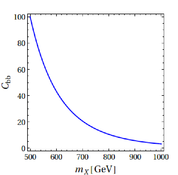
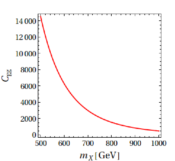
where Kg​g,Kb​b¯K_{gg},K_{b{\bar{b}}} are K-factors, given by Kg​g=1.5,Kb​b¯=1.2K_{gg}=1.5,K_{b{\bar{b}}}=1.2, and Cg​g,Cb​b¯C_{gg},C_{b{\bar{b}}} are parton luminosities. Their values depend on the mass of the resonance, as shown in figure 3, that we generated with the CTEQ5 package [19].
Refer to caption
Refer to caption
Figure 3: The dependence of partonic integrals coefficients Cg​gC_{gg} and Cb​b¯C_{b\bar{b}} at s=13\sqrt{s}=13 TeV on mXm_{X} [19]. In the model considered here X=H,AX=H,A. For example, for mX=750m_{X}=750 GeV one has Cg​g=2131C_{gg}=2131, Cb​b¯=14.6C_{b{\bar{b}}}=14.6; also Cγ​γ≈54C_{\gamma\gamma}\approx 54, Cu​u¯≈1054C_{u\bar{u}}\approx 1054, Cd​d¯≈627C_{d\bar{d}}\approx 627, Cc​c¯≈36C_{c\bar{c}}\approx 36, for s=13\sqrt{s}=13 TeV.

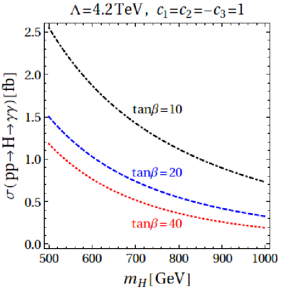
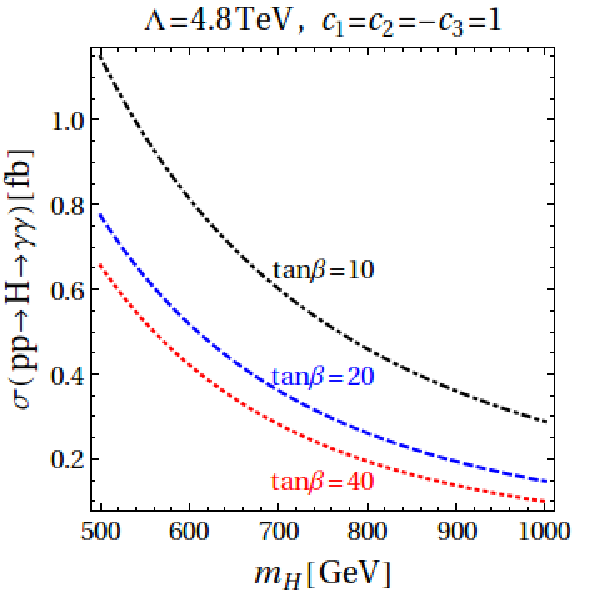
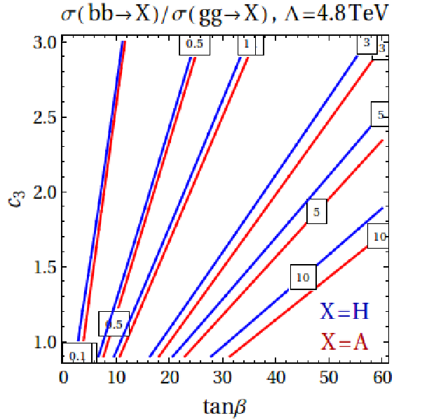
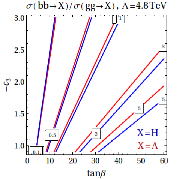
Using the information in figure 3 for the coefficients Cg​gC_{gg} and Cb​b¯C_{b\bar{b}} one can compute the diphoton production cross section for different values of the resonance mass. This dependence is shown in the plots of figure 4, for a fixed scale Λ=4.2\Lambda=4.2 and 4.84.8 TeV of the effective operator and different tan⁡β\tan\beta and c1,2,3c_{1,2,3} 55 5 We keep cjc_{j} close to unity (while freely adjusting Λ\Lambda), otherwise the effective scale of new physics (operator ℒj{\cal L}_{j}) is changed to Λ/|cj|\Lambda/\sqrt{|c_{j}|}.. Both production channels b​b¯b\bar{b} and g​ggg of H,AH,A contribute, see figure 5. In some cases, the cross section can be large, σ∼\sigma\sim few fb, well above its value in the MSSM alone and this can conflict with the latest data [4]. To avoid this situation, as seen in figure 4, a larger mXm_{X} and/or larger Λ\Lambda and/or large tan⁡β\tan\beta may be required, correlated as shown. If the value of σ\sigma is known from experiments and assuming X=H,AX=H,A, these plots together with constraints on SM-like Higgs physics can be used to set stronger bounds on the correlation of Λ\Lambda with tan⁡β\tan\beta and mH,Am_{H,A}. We shall do this shortly for mH,Am_{H,A} in the range 0.5−10.5-1 TeV.

Refer to caption
Refer to caption
Refer to caption
Refer to caption
Figure 4: The diphoton production cross section for fixed Λ\Lambda as a function of the mass mXm_{X} (X=HX=H) for different tan⁡β\tan\beta and coefficients c1,2,3c_{1,2,3} of the effective operators. Similar dependence (nearly identical) exists for X=AX=A. The largest cross section for a given Λ\Lambda is obtained if all c1,2,3≠0c_{1,2,3}\not=0 and have appropriate relative signs (shown). Of individual contributions for the same effective scale, the largest correction to σ\sigma is from ℒ3{\cal L}_{3}, then ℒ1{\cal L}_{1}.
Refer to caption
Refer to caption
Figure 5: Ratios of production cross sections: σ⁡(b​b¯→X)\sigma(b{\bar{b}}\rightarrow X)/σ⁡(g​g→X)\sigma(gg\rightarrow X) for X=HX=H in blue and X=AX=A in red, for c3>0c_{3}\!>\!0 (left plot) and c3<0c_{3}\!<\!0 (right plot). Depending on tan⁡β\tan\beta and |c3||c_{3}| either g​ggg or b​b¯b\bar{b} production mechanism may dominate or they have comparable cross sections. Here we chose mH,A=750m_{H,A}=750 GeV, for illustration.
Refer to caption
Refer to caption
Refer to caption
Refer to caption
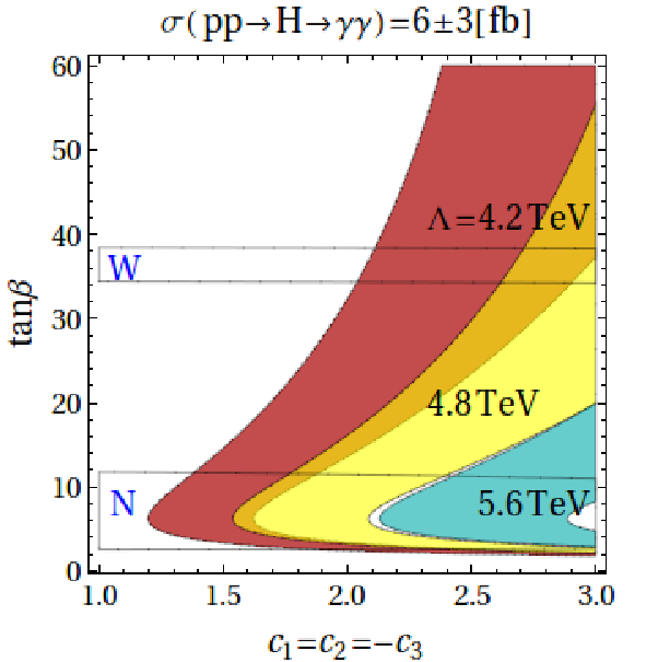
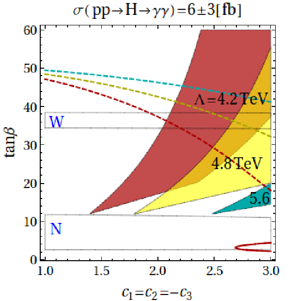
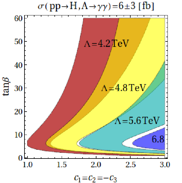
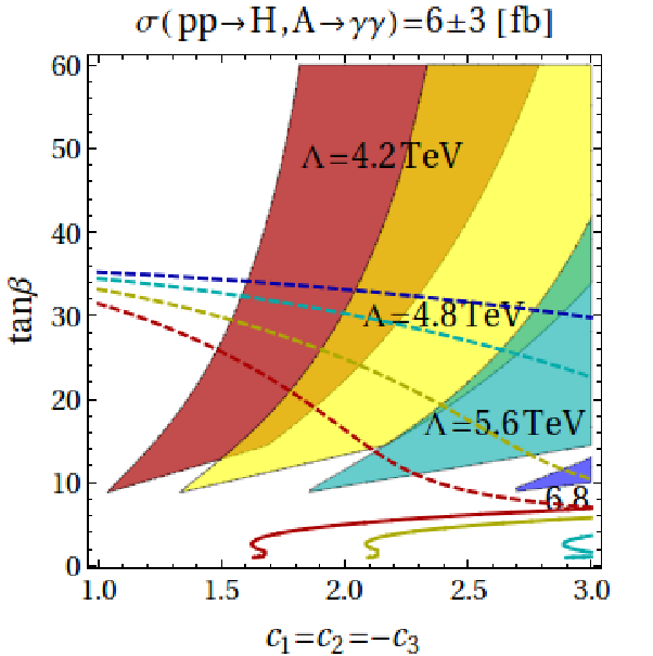
Figure 6: Parameter space for the diphoton cross section σ\sigma, mediated by HH (top) and by both AA, HH, mass degenerate, at mH,A=750m_{H,A}=750 GeV (bottom). Nearly identical plots to HH exist for AA alone. Each coloured area has σ=6±3​fb\sigma=6\pm 3\,{\rm fb} with a fixed Λ\Lambda. Areas of overlapping colours (e.g. red and yellow, shown in orange) correspond to two different Λ\Lambda, (3≤σ≤93\leq\sigma\leq 9). Region “N” corresponds to a narrow resonance ΓH,A≤5\Gamma_{H,A}\leq 5 GeV; region “W” has a wide width of 40≤ΓH,A≤5040\leq\Gamma_{H,A}\!\leq\!50 GeV. For ≤tan⁡β≤3612\!\leq\!\tan\beta\!\leq\!36, ΓH,A\Gamma_{H,A} has intermediate values (fig.2). Region “W” is excluded by the constraint ℛb​b¯≡ΓX→b​b¯/ΓX→γ​γ≤500​(r/5){\cal R}_{b\bar{b}}\equiv\Gamma_{X\rightarrow b\bar{b}}/\Gamma_{X\rightarrow\gamma\gamma}\leq 500(r/5), X=A,HX\!=\!A,H. The plots in the right column have CMS bounds on κγ\kappa_{\gamma} and κg\kappa_{g} applied which excluded the low tan⁡β\tan\beta regions. A dotted (continuous) curve in a colour rules out the area (if present) in the same colour situated above (below) that curve, due to b​b¯b\bar{b} (t​t¯t\bar{t}) searches, respectively [7]. The corresponding region of this “resonance”, for fixed Λ\Lambda, is the area in a given colour below the dotted curve in the same colour, in the right column of plots.

2.4 The dependence of σ\sigma on mH,Am_{H,A} and the missing 750 GeV “resonance”

As seen in the previous section, ℒ1,2,3{\cal L}_{1,2,3} may provide a diphoton production cross section that is as large as few fb, as initially reported by ATLAS/CMS [1], at mX=750m_{X}=750 GeV, (X=H,AX=H,A), now ruled out by recent additional data [4]. In the following we first detail the exclusion limits on the scale Λ\Lambda, correlated with tan⁡β\tan\beta, from the absence of this resonance. We then consider the general case of varying 0.50.5 TeV≤mH,A≤1\leq m_{H,A}\leq 1 TeV and explore the dependence of σ\sigma on mH,Am_{H,A}, Λ\Lambda and tan⁡β\tan\beta, under the experimental constraints from the SM-like higgs couplings h​g​ghgg and h​γ​γh\gamma\gamma and from b​b¯b\bar{b} and t​t¯t\bar{t} searches. Both production channels of X=H,AX=H,A are included and either of these may dominate (figure 5).

Figure 6 shows the parameter space giving the initially found σ(pp→H,A→γγ)=6±3\sigma(pp\rightarrow H,A\rightarrow\gamma\gamma)=6\pm 3 fb at mX=750m_{X}=750 GeV, mediated by HH or AA or both (mass degenerate case66 6 In the decoupling limit we use, valid for mA=750m_{A}=750 GeV, the mass splitting δ​m\delta m between AA and HH can be neglected mH2=mA2+mZ2​sin2⁡[2​β]m_{H}^{2}=m_{A}^{2}+m_{Z}^{2}\sin^{2}[2\beta], so δ​m≤2\delta m\leq 2 GeV for tan⁡β>3\tan\beta>3 and decreases further at larger tan⁡β\tan\beta.). The allowed parameter space is similar for AA and HH. In this figure the relative signs of |cj|∼1|c_{j}|\sim 1 were chosen to maximise the diphoton production for given Λ\Lambda. Note that the effective cutoff of an operator is ultimately Λ/|cj|\Lambda/\sqrt{|c_{j}|}.

Narrow resonance:   For low 2≤tan⁡β≤122\leq\tan\beta\leq 12 (figures 2, 6) one has a narrow width, ΓH,A≤5\Gamma_{H,A}\leq 5 GeV. For tan⁡β≤8\tan\beta\leq 8, the g​ggg production channel of H,AH,A dominates; for 8≤tan⁡β≤128\leq\tan\beta\leq 12 the b​b¯b\bar{b} channel is also relevant (figure 5).

Let us see the effect of the constraints from the SM-like higgs (hh) rates. In figure 6 the low tan⁡β\tan\beta region contributes to h→γ​γh\rightarrow\gamma\gamma (photons) and h→g​gh\rightarrow gg (gluons) and can even enhance (reduce) the rate of h→γ​γh\rightarrow\gamma\gamma beyond the SM value for negative (positive) c1,2c_{1,2}, respectively [20]77 7 This is due to coefficients c^γ​γ\hat{c}_{\gamma\gamma} or cγ​γc_{\gamma\gamma} which contribute at low tan⁡β\tan\beta, see eqs.(6), (9) for α→β−π/2\alpha\rightarrow\beta-\pi/2.. Define by κγ\kappa_{\gamma} and κg\kappa_{g} the scaling coefficients of the amplitude of the SM-like higgs couplings to γ​γ\gamma\gamma and g​ggg; then one has [21] (see also [22, 23]):

CMS,  68%​CL:\displaystyle{\rm CMS,}\,\,68\%{\rm CL:} κγ=0.965±0.175,κg=0.835±0.105\displaystyle\kappa_{\gamma}=0.965\pm 0.175,\hskip 20.00003pt\kappa_{g}=0.835\pm 0.105 (15)
ATLAS,  68%​CL:\displaystyle{\rm ATLAS,}\,\,68\%{\rm CL:} κγ=1.2±0.15,κg=1.04±0.14\displaystyle\kappa_{\gamma}=1.2\pm 0.15,\hskip 10.00002pt\,\,\,\hskip 20.00003pt\kappa_{g}=1.04\pm 0.14 (16)

We used the CMS constraint in fig. 6 at 95%95\% CL, with κj2=Γh→j​j/Γh→j​jS​M\kappa_{j}^{2}=\Gamma_{h\rightarrow jj}/\Gamma_{h\rightarrow jj}^{SM}, j=γ,gj=\gamma,g. As a result, 2≤tan⁡β≤102\leq\tan\beta\leq 10 or so is in conflict with these constraints from hh decays and this region, largely overlapping with our narrow width regime, is ruled out. Further, t​t¯t\bar{t} searches also rule out some parameter space close to 1≤tan⁡β<81\leq\tan\beta<8 but the bound found is in general weaker than the above bounds from hh signals88 8 The bound used for t​t¯t\bar{t} searches is σ⁡(p​p→X→t​t¯)<2250\sigma(pp\rightarrow X\rightarrow t\bar{t})<2250 fb (13 TeV), see Table 1 in [7].. As a result, the parametric region in figure 6 corresponding to this narrow “resonance” is a small region at the tip of each coloured area of fixed Λ\Lambda with tan⁡β≈10−12\tan\beta\!\approx\!10-12.

Broad resonance:    The region 34≤tan⁡β≤3834\leq\tan\beta\leq 38 (40≤ΓH,A≤5040\leq\Gamma_{H,A}\leq 50 GeV, fig.2) marked as “W” in figs. 6, where the b​b¯b\bar{b} production mechanism dominates (if |c3|≈1−2|c_{3}|\approx 1-2, fig.5), is ruled out by constraints such as those in Table 1, of which ℛb​b¯<500{\cal R}_{b\bar{b}}<500 is the strongest. Further, b​b¯b\bar{b} searches with a cross section bound ≤5\leq 5 pb at 13 TeV (Table 1 in [7]) are also marked in figs.6, with a dotted curve in a given colour that rules out any area in the same colour situated above that curve. This leaves a parametric area bordered by tan⁡β≤25\tan\beta\leq 25 with ΓX≤25\Gamma_{X}\leq 25 GeV (tan⁡β≤18\tan\beta\leq 18, ΓX≤12\Gamma_{X}\leq 12 GeV) for σ≈3\sigma\approx 3 fb (σ≈9\sigma\approx 9 fb) respectively, for mass degenerate AA and HH and Λ/|cj|\Lambda/\sqrt{|c_{j}|} fixed.

With this resonance now ruled out, one must then exclude its parametric region bordered by 10≤tan⁡β≤2510\leq\tan\beta\leq 25 (10≤tan⁡β≤1810\leq\tan\beta\leq 18) for σ≈3\sigma\approx 3 fb (σ≈9\sigma\approx 9 fb), respectively and demand the effective scale be larger than Λ/|cj|≈4.2\Lambda/\sqrt{|c_{j}|}\approx 4.2 TeV. We checked that similar bounds apply for mildly different values of c1,2,3c_{1,2,3} and from unity. These bounds are relevant provided that all ℒ1,2,3{\cal L}_{1,2,3} in eq.(3) contribute. Since ℒ3{\cal L}_{3} is the dominant contribution, if c3=0c_{3}=0 then one has a much smaller diphoton cross section. If c2=0c_{2}=0 (or c1=0c_{1}=0) and c3≠0c_{3}\not=0 i.e. only ℒ1,3{\cal L}_{1,3} (ℒ2,3{\cal L}_{2,3}) are present, total σ\sigma is again reduced; one may still reach σ∼3\sigma\sim 3 fb by compensating with an increase of the remaining coefficients, but then Λ/|cj|\Lambda/\sqrt{|c_{j}|} may become too low for a reliable effective expansion.

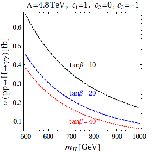
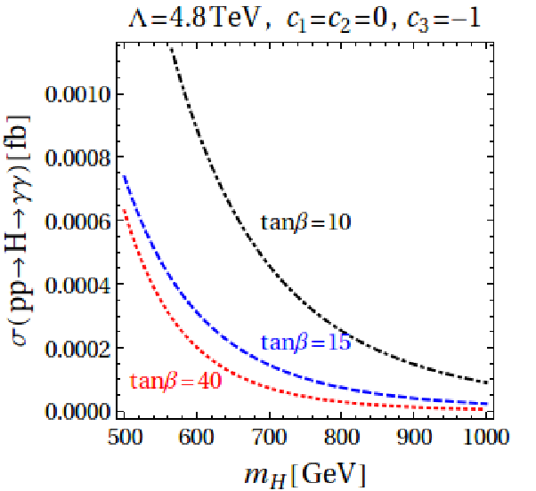
We return now to a general case of varying mH,Am_{H,A} in the range 0.50.5 TeV ≤mH,A≤1\leq\!m_{H,A}\!\leq 1 TeV. Figure 7 shows the dependence of the diphoton cross section σ\sigma on mH,Am_{H,A} and tan⁡β\tan\beta, under the experimental constraints from h​g​ghgg and h​γ​γh\gamma\gamma couplings and b​b¯b\bar{b}, t​t¯t\bar{t} searches. The cross section bounds for the b​b¯b\bar{b} and t​t¯t\bar{t} searches depend on mH,Am_{H,A}; we used the observed values (95%95\% CL) for b​b¯b\bar{b} searches of figure 6 in [26] and for t​t¯t\bar{t} searches of figure 2 in [27], for the range of mXm_{X} considered in our figure 7. These values were scaled to s=13\sqrt{s}=13 TeV. The dependence of the parton coefficients on mH,Am_{H,A} is also included (see figure 3).

Large values of diphoton cross section σ∼0.1−1\sigma\sim 0.1-1 fb (well above the MSSM value) are obtained when both ℒ3{\cal L}_{3} and ℒ1{\cal L}_{1} are present, for Λ=4.8\Lambda=4.8 TeV (right plot in fig.7). For |c3||c_{3}| only mildly different from unity |c3|∼1.3|c_{3}|\sim 1.3 or if also c2≠0c_{2}\not=0, then σ\sigma increases further from the values shown. Unlike for the 750750 GeV “resonance”, there are now regions of low tan⁡β<10\tan\beta<10 with a large diphoton production such as: σ∼1\sigma\sim 1 fb for mH,A∼550−650m_{H,A}\sim 550-650 GeV, or σ∼0.4\sigma\sim 0.4 fb for mH,A∼1m_{H,A}\sim 1 TeV, that pass all the above constraints99 9 The low tan⁡β\tan\beta region may also be interesting for the naturalness issue, see later.. Increasing Λ\Lambda above ∼5\sim 5 TeV or considering instead only individual operators, e.g. dominant ℒ3{\cal L}_{3} (left plot in figure 7), can reduce σ\sigma significantly. This ends our analysis of the diphoton cross section for mH,Am_{H,A} in the range 0.5−10.5-1 TeV.

ℛZ​Z{\cal R}_{ZZ} ℛZ​γ{\cal R}_{Z\gamma} ℛW​W{\cal R}_{WW} ℛt​t¯{\cal R}_{t\bar{t}} ℛb​b¯{\cal R}_{b\bar{b}} ℛg​g{\cal R}_{gg}
6​(r/5)6(r/5) 6​(r/5)6(r/5) 20​(r/5)20(r/5) 300​(r/5)300(r/5) 500​(r/5)500(r/5) 1300​(r/5)1300(r/5)
Table 1: Upper bounds on the partial widths ℛa​b=ΓX→a​b/ΓX→γ​γ{\cal R}_{ab}=\Gamma_{X\rightarrow ab}/\Gamma_{X\rightarrow\gamma\gamma}, (X=H,AX=H,A), obtained from 8 TeV data scaled to 13 TeV, with r=σ13​T​e​V/σ8​T​e​V≈5r=\sigma_{\rm 13TeV}/\sigma_{\rm 8TeV}\approx 5  and a wide resonance ΓH,A=45\Gamma_{H,A}=45 GeV [7]. They apply at large tan⁡β\tan\beta. ℛb​b¯{\cal R}_{b\bar{b}} is the strongest bound.
Refer to caption
Refer to caption
Figure 7: Parameter space for different values of the diphoton cross section σ\sigma, mediated by both AA, HH (mass degenerate) for a varying mass mH,Am_{H,A} with Λ=4.8\Lambda=4.8 TeV and c1,2=0c_{1,2}=0, c3=−1c_{3}=-1 (left) and c1=−c3=1c_{1}=-c_{3}=1, c2=0c_{2}=0 (right). The red regions in the left plot have σ\sigma in the range shown while in the right plot, their left edge has σ\sigma larger by 0.030.03 fb from the values shown. The partonic integral coefficients dependence on mH,Am_{H,A} is included. The CMS bounds on κγ\kappa_{\gamma} and κg\kappa_{g} excluded a small low tan⁡β<6\tan\beta<6 regions. The dotted curve (in blue) corresponds to a bound from b​b¯b\bar{b} searches (observed values, see figure 6 in [26]). The t​t¯t\bar{t} searches bound (observed values, see figure 2 in [27]) is also imposed but for the cases considered here for c1,2,3c_{1,2,3} does not constrain the parameter space. The allowed parametric region is then the area below the dotted curve.

3 Microscopic models for ℒ1,2,3{\cal L}_{1,2,3} and higgs mass corrections

Having seen the role of ℒ1,2,3{\cal L}_{1,2,3} on the diphoton cross section, we now explain their possible origin in a renormalizable model. We also address their effect on the higgs sector masses.

3.1 Microscopic origin of effective operator(s) ℒ1,2,3{\cal L}_{1,2,3}

ℒ1,2,3{\cal L}_{1,2,3} may be generated in the MSSM with additional states with mass of order Λ\Lambda. To see this, consider a massive gauge singlet SS that couples to the higgs and gauge sector as in:

δL=∫d4θS†S+{∫d2θ[μH1.H2+λSH1.H2+12M1S2+f(S)Tr(𝒲αWα)]+h.c}\displaystyle\delta L\!\!=\!\!\int\!d^{4}\theta\,S^{\dagger}S+\Big\{\!\!\int\!d^{2}\theta\Big[\mu H_{1}.H_{2}\!+\!\lambda\,S\,H_{1}.H_{2}\!+\frac{1}{2}\,M_{1}S^{2}+f(S)\mbox{Tr}({\cal W}^{\alpha}W_{\alpha})\Big]\!+\!\textsf{h.c}\Big\} (17)

f⁡(S)=S/M2f(S)=S/M_{2} is a gauge kinetic function of a SM subgroup and M2M_{2} some high mass scale. To generate all ℒ1,2,3{\cal L}_{1,2,3} the coupling to the gauge sector is extended to S​U​(3)×S​U​(2)L×U​(1)YSU(3)\times SU(2)_{L}\times U(1)_{Y}. We integrate out the superfield SS via its eqs of motion and find after some algebra and consistent truncation of higher orders

δ​L\displaystyle\delta L\!\!\! =\displaystyle= ∫d4θ[2|λM1|2|H1.H2|2]\displaystyle\!\!\!\!\int d^{4}\theta\,\Big[2\,\Big|\frac{\lambda}{M_{1}}\Big|^{2}\,|H_{1}.H_{2}|^{2}\Big] (18)
+∫d2θ[μH1.H2−λ22​M1(H1.H2)2−λM1​M2(H1.H2)Tr(WαWα)]+h.c+𝒪(1/M13)\displaystyle\!\!\!\!\!\!\!\!\!\!\!\!\!\!\!\!\!+\int\!\!d^{2}\theta\Big[\mu\,H_{1}.H_{2}-\frac{\lambda^{2}}{2\,M_{1}}\,(H_{1}.H_{2})^{2}\!-\frac{\lambda}{M_{1}\,M_{2}}(H_{1}.H_{2})\,\mbox{Tr}(W^{\alpha}W_{\alpha})\Big]\!+\!\textsf{h.c}\!+\!{\cal O}(1/M_{1}^{3})\hskip 10.00002pt

In the rhs of the above equation there are two more terms: −1/(2M1M22)(TrW2))2|F-1/(2M_{1}M_{2}^{2})(\mbox{Tr}W^{2}))^{2}|_{F} and also 2λ/(M12M2)(H1.H2)†TrW2|D2\lambda/(M_{1}^{2}M_{2})(H_{1}.H_{2})^{\dagger}\mbox{Tr}W^{2}|_{D}; since we choose M2≥M1M_{2}\geq M_{1}, they are sub-leading, O⁡(1/M13)O(1/M_{1}^{3}), and can be ignored. The last line in eq.(18) shows our operators of d=6d=6 and d=5d=5 generated simultaneously when integrating SS. However eq.(17) does not yet provide a UV complete, renormalizable setup, since it still contains a d=5d=5 effective operator: (S/M2)​Tr​(Wα​Wα)|F(S/M_{2})\,\mbox{Tr}\,(W^{\alpha}W_{\alpha})|_{F}. One possibility is that this operator is generated if SS has additional, renormalizable couplings to massive vector-like states under the SM gauge group, of mass 𝒪⁡(M2){\cal O}(M_{2}), as shown in diagram (1) of figure 8. Integrating out the vector-like states then generates this remaining operator1010 10 (S/M2)​Tr​Wα​Wα|F(S/M_{2})\,\mbox{Tr}\,W^{\alpha}W_{\alpha}|_{F} is a moduli-dependent gauge kinetic term, generic in supergravity or string theory.. We thus have a microscopic origin of ℒ1,2,3{\cal L}_{1,2,3}.

Refer to caption
Figure 8: Diagrams generating the d=6d=6 operator (H1.H2)Tr(WαWα)|F(H_{1}.H_{2})\,\mbox{Tr}\,(W^{\alpha}W_{\alpha})|_{F} at one-loop level. Diagram (1) corresponds to the approach in eqs.(17), (18), with a loop of vector-like states of mass ∝M2\propto M_{2} that generate (S/M2)​Tr​(Wα​Wα)|F(S/M_{2})\mbox{Tr}(W^{\alpha}W_{\alpha})|_{F} of eq.(17), while (classical) integration of SS generates the needed d=6d=6 operator. Diagram (2) (plus another one as (2) but with Q↔UcQ\leftrightarrow U^{c}, Q¯↔U¯c\overline{Q}\leftrightarrow\overline{U}^{c}) show how to generate the d=6d=6 operator in one stage, without a massive singlet SS. A large number of vector-like states can compensate the loop suppression.

Eq.(18) also contains a d=6d=6 operator |H1.H2|2D|H_{1}.H_{2}|^{2}_{D} which brings a negative correction to the SM-like Higgs mass δmh2=−4v2|λ|2μ2/Λ2+𝒪(1/tan2β)\delta m_{h}^{2}=-4v^{2}|\lambda|^{2}\mu^{2}/\Lambda^{2}+{\cal O}(1/\tan^{2}\beta) [18] (for M1=ΛM_{1}=\Lambda); this correction is less relevant (being sub-leading to that of eq.(21), see later). Finally, taking M1∼M2∼ΛM_{1}\sim M_{2}\sim\Lambda and comparing eq.(18) to (3), we identify λ=cj/2\lambda=c_{j}/2 and c0=−λ2/2=−cj2/8c_{0}=-\lambda^{2}/2=-c_{j}^{2}/8.

Another way to generate (H1.H2)Tr(WαWα)F(H_{1}.H_{2})\,\mbox{Tr}(W^{\alpha}W_{\alpha})_{F} is at one-loop, without a massive singlet. One considers only copies of massive vector-like states as in diagram (2) of fig.8.

To conclude, a heavy diphoton resonance (X=H,AX=H,A) of large cross section is present if SM-charged, massive vector-like states (and possibly a singlet) are present beyond MSSM; after decoupling, they generate ℒ1,2,3{\cal L}_{1,2,3}. Other ways to generate the d=6d=6 operator(s) may exist. The vector-like states have a significant impact on the gauge couplings unification at one-loop, unless they are complete S​U​(5)SU(5) multiplets [28].

3.2 Implications for Higgs sector masses

Unlike the “gluon” operator ℒ3{\cal L}_{3}, the “electroweak” operators ℒ1,2{\cal L}_{1,2} of eq.(3) also impact on the higgs masses mh,H2=Mh,H2+Δ​mh,H2m_{h,H}^{2}=M_{h,H}^{2}+\Delta m_{h,H}^{2}. Here Mh,HM_{h,H} denote the MSSM value. We find1111 11 using the first ref in [18] and adding a one-loop effect, too (top Yukawa).

Δ​mh,H2=8​ρΛ2​[g12​c1+g22​c2]+𝒪⁡[1Λ3]\displaystyle\Delta m_{h,H}^{2}=\frac{8\rho}{\Lambda^{2}}\Big[g_{1}^{2}c_{1}+g_{2}^{2}c_{2}\Big]+{\cal O}\!\Big[\frac{1}{\Lambda^{3}}\!\Big]\, (19)

where

ρ=v432​sin⁡2​β​[1±14​w​[8​mA2−(4+3​δ)​mZ2+6​δ​mZ2​cos⁡2​β+3​(4​mA2−δ​mZ2)​cos⁡4​β]]\displaystyle\rho=\frac{v^{4}}{32}\,\sin 2\beta\,\Big[1\pm\frac{1}{4\,\sqrt{w}}\big[8m_{A}^{2}-(4+3\delta)m_{Z}^{2}+6\delta m_{Z}^{2}\cos 2\beta+3(4m_{A}^{2}-\delta m_{Z}^{2})\cos 4\beta\big]\Big] (20)

and w=[(mA2−mZ2)​cos⁡2​β+δ​mZ2​sin2⁡β]2+sin2⁡2​β​(mA2+mZ2)2w=[(m_{A}^{2}-m_{Z}^{2})\,\cos 2\beta+\delta\,m_{Z}^{2}\,\sin^{2}\beta]^{2}+\sin^{2}2\beta\,(m_{A}^{2}+m_{Z}^{2})^{2}; the upper (lower) signs correspond to hh (HH) and δ\delta is shown in Appendix B. These corrections bring a modest increase of the SM-like higgs mass Δ​mh∼1​GeV\Delta m_{h}\sim 1\textsf{GeV} for c1,2=𝒪⁡(1)c_{1,2}={\cal O}(1), with a largest value for small tan⁡β\tan\beta, with little dependence on mAm_{A}. An even smaller correction is found for mHm_{H}. The mass of the CP-odd Higgs boson is also modified, see eq.(B-2). These corrections have little impact on the previous diphoton analysis.

As we saw in the previous sub-section, a leading d=5d=5 operator

ℒ0\displaystyle{\cal L}_{0} =\displaystyle= c0Λ∫d2θ(H1.H2)2+h.c.\displaystyle\frac{c_{0}}{\Lambda}\int d^{2}\theta\,\,(H_{1}.H_{2})^{2}+\mbox{h.c.} (21)

may also be generated from the UV complete (renormalizable) model, without direct contribution to the diphoton cross section. Its correction to the higgs mass is [16, 18]

Δ​mh,H2=[2​μ​c0Λ]​ρ1+[2​μ​c0Λ]2​ρ2+𝒪⁡[1Λ3]\displaystyle\Delta m_{h,H}^{2}=\left[2\mu\,\frac{c_{0}}{\Lambda}\right]\rho_{1}+\left[2\mu\frac{c_{0}}{\Lambda}\right]^{2}\rho_{2}+{\cal O}\!\Big[\frac{1}{\Lambda^{3}}\!\Big]\, (22)

where ρ1,2\rho_{1,2} are shown in eq.(B-4). With c0​μ>0c_{0}\,\mu>0, a numerical analysis shows a significant increase of mhm_{h} for small tan⁡β<10\tan\beta<10, by as much as ≈10\approx 10 GeV [16]. This increase can reduce the amount of EW scale fine tuning by a significant factor [16, 24] relative to its MSSM value at low tan⁡β\tan\beta region (which is an otherwise very fine tuned MSSM region).

4 Conclusions

Current searches for “new physics” at the LHC bring increasingly strong constraints on the MSSM-like models. Their parameter space becomes smaller, with negative implications for their naturalness. However, simple extensions of their minimal higgs sector, parametrised by effective (supersymmetric) operators, relax the parameter space or even improve naturalness. We studied the constraints on such operators that can enhance dramatically the couplings of the higgs sector to SM gauge bosons and thus the heavy diphoton production.

Minimal models (MSSM) have a small diphoton cross section at large mH,Am_{H,A}, unless one is fine-tuning the parameters. We identified leading operators of dimension d=6d\!=\!6 in the higgs sector ℒj∼cj/Λ2(H1.H2)Tr(WαWα)j|F{\cal L}_{j}\sim c_{j}/\Lambda^{2}\,(H_{1}.H_{2})\mbox{Tr}(W^{\alpha}W_{\alpha})_{j}|_{F}, j=1,2,3j\!=\!1,2,3, cj=𝒪⁡(1)c_{j}={\cal O}(1), that enhance the couplings to SM gauge bosons, with ℒ3{\cal L}_{3} having the dominant effects. For mH,Am_{H,A} in the range 0.50.5 TeV≤mH,A≤1\leq m_{H,A}\leq 1 TeV, the combination ℒ1+ℒ3{\cal L}_{1}+{\cal L}_{3} can lead to a large diphoton production σ∼0.1−1\sigma\sim 0.1-1 fb, well above the MSSM value. The analysis included both g​ggg and b​b¯b\bar{b} production mechanisms (of X=H,AX\!=\!H,A) and either of these may dominate. We examined the correlation between the diphoton cross section σ\sigma and the values of mXm_{X}, Λ\Lambda and tan⁡β\tan\beta, under the experimental constraints from SM-like higgs couplings h​g​ghgg and h​γ​γh\gamma\gamma (due to mixing) and from b​b¯b\bar{b} and t​t¯t\bar{t} searches. These give Λ/|cj|>4.8\Lambda/\sqrt{|c_{j}|}>4.8 TeV where the effective approach can still be trusted, for mH,Am_{H,A} between 0.5−10.5-1 TeV.

Regarding the initially claimed resonance at mX=750m_{X}\!=\!750 GeV with even larger σ\sigma (few fb), this could be reached if all ℒ1,2,3{\cal L}_{1,2,3} contribute. Recent data ruled out this resonance, then not all ℒ1,2,3{\cal L}_{1,2,3} are simultaneously present or the scale Λ/|cj|\Lambda/\sqrt{|c_{j}|} is larger than 4−54-5 TeV.

We showed how to generate the d=6d=6 effective operator(s) from a UV complete (renormalizable) theory. This is possible by integrating out additional massive SM vector-like states beyond the MSSM spectrum, and eventually a massive singlet too, of mass 𝒪⁡(Λ){\cal O}(\Lambda). An additional d=5d=5 operator in the higgs sector may also be generated at the same time, that does not affect directly the diphoton production, but may improve naturalness.

—————————–

Appendix:

A Loop functions and couplings

In this section we present the expressions of the coefficients a..l​o​o​pa_{\bf..}^{loop}, b..l​o​o​pb_{..}^{loop}, c..l​o​o​pc_{..}^{loop}, used in the text (section 2.1). To compute them and to fix the notation, we need the couplings of MSSM fields h,Hh,H, AA to fermions and gauge bosons. These are, in a standard notation

−Δ​ℒ\displaystyle-\Delta{\cal L} =\displaystyle= kt​mtv​h​t¯​t+kb​mbv​h​b¯​b+2​mW2v​(kw​h+k~w​H)​W+μ​Wμ−\displaystyle k_{t}\,\frac{m_{t}}{v}\,h\overline{t}\,t+k_{b}\,\frac{m_{b}}{v}\,h\overline{b}\,b+\frac{2m_{W}^{2}}{v}\,(k_{w}h+\tilde{k}_{w}H)W^{+\mu}W^{-}_{\mu} (A-1)
+k~t​mtv​H​t¯​t+k~b​mbv​H​b¯​b+i​k¯t​mtv​A​t¯​γ5​t+i​k¯b​mbv​A​b¯​γ5​b\displaystyle+\tilde{k}_{t}\,\frac{m_{t}}{v}\,H\,\overline{t}\,t+\tilde{k}_{b}\,\frac{m_{b}}{v}\,H\,\overline{b}\,b+i\bar{k}_{t}\,\frac{m_{t}}{v}\,A\,\overline{t}\,\gamma^{5}t+i\bar{k}_{b}\,\frac{m_{b}}{v}\,A\,\overline{b}\,\gamma^{5}b

where

kt\displaystyle k_{t} =\displaystyle= cos⁡αsin⁡β,kb=−sin⁡αcos⁡β,kw=sin⁡(β−α)\displaystyle\frac{\cos\alpha}{\sin\beta},\hskip 10.00002ptk_{b}=-\frac{\sin\alpha}{\cos\beta},\hskip 10.00002ptk_{w}=\sin(\beta-\alpha)
k~t\displaystyle\tilde{k}_{t} =\displaystyle= sin⁡αsin⁡β,k~b=cos⁡αcos⁡β,k~w=cos⁡(β−α),\displaystyle\frac{\sin\alpha}{\sin\beta},\hskip 10.00002pt\,\tilde{k}_{b}=\frac{\cos\alpha}{\cos\beta},\hskip 20.00003pt\tilde{k}_{w}=\cos(\beta-\alpha),
k¯t\displaystyle\bar{k}_{t} =\displaystyle= cot⁡β,k¯b=−tan⁡β.\displaystyle\cot\beta,\hskip 20.00003pt\bar{k}_{b}=-\tan\beta. (A-2)

Here α\alpha is the mixing angle in the Higgs sector. In this paper we work in the decoupling limit (mAm_{A} large). Then α→β−π/2\alpha\rightarrow\beta-\pi/2 and kt,b,w=1k_{t,b,w}=1 while k~t=−cot⁡β\tilde{k}_{t}=-\cot\beta, k~b=tan⁡β\tilde{k}_{b}=\tan\beta, k~w=0\tilde{k}_{w}=0. Then we find the coefficients of the effective operators in eqs.(9), (10), as follows [25]

ag​gl​o​o​p\displaystyle a_{gg}^{loop}\!\!\!\! =\displaystyle= k¯t​A¯g(t)+k¯b​A¯g(b)≈(0.0771+0.7064​i)​cot⁡β−(0.00281+0.00194​i)​tan⁡β\displaystyle\!\!\!\bar{k}_{t}\,{\bar{A}}_{g}^{(t)}+\bar{k}_{b}{\bar{A}}_{g}^{(b)}\approx(0.0771+0.7064i)\cot\beta-(0.00281+0.00194i)\tan\beta\,
aγ​γl​o​o​p\displaystyle\!\!\!a_{\gamma\gamma}^{loop}\!\!\! =\displaystyle= k¯w​A¯γ(W)+k¯t​A¯γ(t)+k¯b​A¯γ(b)≈(+1.256​i)​cot⁡β+(−0.00086​i)​tan⁡β\displaystyle\!\!\!\!\bar{k}_{w}\,{\bar{A}}_{\gamma}^{(W)}\!+\!\bar{k}_{t}\,{\bar{A}}_{\gamma}^{(t)}\!+\!\bar{k}_{b}\,{\bar{A}}_{\gamma}^{(b)}\approx\!(0.13702\!+\!1.256i)\cot\beta\!+\!(0.00125\!-\!0.00086i)\tan\beta
aγ​zl​o​o​p\displaystyle a_{\gamma z}^{loop} =\displaystyle= az​zl​o​o​p=aw​wl​o​o​p=0.\displaystyle a_{zz}^{loop}=a_{ww}^{loop}=0.

and

bg​gl​o​o​p\displaystyle b_{gg}^{loop}\!\!\! =\displaystyle= k~t​A~g(t)+k~b​A~g(b)≈−(0.441+1.112​i)​cot⁡β+(−0.00538+0.00387​i)​tan⁡β\displaystyle\!\!\!\tilde{k}_{t}\,{\tilde{A}}_{g}^{(t)}+\tilde{k}_{b}{\tilde{A}}_{g}^{(b)}\approx-(0.441+1.112i)\cot\beta+(-0.00538+0.00387i)\tan\beta\,
bγ​γl​o​o​p\displaystyle b_{\gamma\gamma}^{loop}\!\!\!\! =\displaystyle= k~wA~γ(W)+k~tA~γ(t)+k~bA~γ(b)≈−(0.783+1.98i)cotβ+(−+0.00172i)tanβ\displaystyle\!\!\!\tilde{k}_{w}\,{\tilde{A}}_{\gamma}^{(W)}\!+\tilde{k}_{t}\,{\tilde{A}}_{\gamma}^{(t)}\!+\!\tilde{k}_{b}\,{\tilde{A}}_{\gamma}^{(b)}\approx\!-(0.783+1.98i)\cot\beta+(-0.00239\!+0.00172i)\tan\beta
bγ​zl​o​o​p\displaystyle b_{\gamma z}^{loop} =\displaystyle= k~t​A~γ​z(t)+k~b​A~γ​z(b)≈(0.12513+0.32821​i)​cot⁡β+(0.00103−0.000043​i)​tan⁡β\displaystyle\tilde{k}_{t}\tilde{A}^{(t)}_{\gamma z}+\tilde{k}_{b}\tilde{A}^{(b)}_{\gamma z}\approx(0.12513+0.32821i)\cot\beta+(0.00103-0.000043i)\tan\beta
bw​wl​o​o​p\displaystyle b_{ww}^{loop} =\displaystyle= bz​zl​o​o​p=0.\displaystyle b_{zz}^{loop}=0. (A-3)

and finally

cg​gl​o​o​p\displaystyle c_{gg}^{loop}\!\!\!\! =\displaystyle= kt​Ag(t)+kb​Ag(b)≈0.970+0.0894​i\displaystyle\!\!\!k_{t}\,A_{g}^{(t)}+k_{b}\,A_{g}^{(b)}\approx 0.970+0.0894i\, (A-4)
cγ​γl​o​o​p\displaystyle c_{\gamma\gamma}^{loop}\!\!\! =\displaystyle= kw​Aγ(W)+kt​Aγ(t)+kb​Aγ(b)≈−6.51+0.0397​i\displaystyle\!\!\!k_{w}A_{\gamma}^{(W)}+k_{t}\,A_{\gamma}^{(t)}+k_{b}\,A_{\gamma}^{(b)}\approx-6.51+0.0397i\, (A-5)

where coefficients A().A^{()}_{.} are one-loop form factors, presented below.

For hh one has the following form factors

Ag(ξ)\displaystyle A_{g}^{(\xi)} =\displaystyle= 34​A1/2​(τξ),ξ=t,b.\displaystyle\frac{3}{4}A_{1/2}(\tau_{\xi}),\hskip 10.00002pt\hskip 20.00003pt\xi=t,b. (A-6)
Aγ(ξ)\displaystyle A_{\gamma}^{(\xi)} =\displaystyle= Nc​Qξ2​A1/2​(τξ),ξ=t,b.\displaystyle N_{c}Q_{\xi}^{2}A_{1/2}(\tau_{\xi}),\hskip 10.00002pt\,\,\xi=t,b. (A-7)
Aγ(W)\displaystyle A_{\gamma}^{(W)} =\displaystyle= A1​(τW)\displaystyle A_{1}(\tau_{W}) (A-8)
AZ​γ(W)\displaystyle{A}_{Z\gamma}^{(W)} =\displaystyle= cos⁡θw​A1​(τW,λW)\displaystyle\cos\theta_{w}\,A_{1}(\tau_{W},\lambda_{W}) (A-9)
AZ​γ(t)\displaystyle{A}_{Z\gamma}^{(t)} =\displaystyle= Nc​Qtcos2⁡θw​(2​T3(t)−4​Qt​sin2⁡θw)cos⁡θw​A1/2​(τt,λt)\displaystyle\frac{N_{c}Q_{t}}{\cos^{2}\theta_{w}}\frac{(2T_{3}^{(t)}-4Q_{t}\sin^{2}\theta_{w})}{\cos\theta_{w}}A_{1/2}(\tau_{t},\lambda_{t}) (A-10)

and for HH

A~g(ξ)\displaystyle\hskip 20.00003pt\hskip 20.00003pt\hskip 20.00003pt\hskip 20.00003pt{\tilde{A}}_{g}^{(\xi)} =\displaystyle= 34​A1/2​(τ~ξ),ξ=t,b.\displaystyle\frac{3}{4}A_{1/2}({\tilde{\tau}}_{\xi}),\hskip 20.00003pt\hskip 20.00003pt\xi=t,b. (A-11)
A~γ(ξ)\displaystyle{\tilde{A}}_{\gamma}^{(\xi)} =\displaystyle= Nc​Qξ2​A1/2​(τ~ξ),ξ=t,b.\displaystyle N_{c}Q_{\xi}^{2}A_{1/2}(\tilde{\tau}_{\xi}),\hskip 20.00003pt\xi=t,b. (A-12)
A~γ​z(ξ)\displaystyle\tilde{A}_{\gamma z}^{(\xi)} =\displaystyle= Nc​Qξcos⁡θw​(2​T3(ξ)−4​Qξ​sin2⁡θw)​A1/2​(τ~ξ,λξ),ξ=t,b.\displaystyle\frac{N_{c}Q_{\xi}}{\cos\theta_{w}}(2T_{3}^{(\xi)}-4Q_{\xi}\sin^{2}\theta_{w})A_{1/2}(\tilde{\tau}_{\xi},\lambda_{\xi}),\hskip 10.00002pt\xi=t,b.\hskip 20.00003pt\,\, (A-13)

and for AA:

A¯g(ξ)\displaystyle\bar{A}_{g}^{(\xi)} =\displaystyle= 34​A¯1/2​(τ¯ξ),ξ=t,b.\displaystyle\frac{3}{4}\bar{A}_{1/2}(\bar{\tau}_{\xi}),\hskip 20.00003pt\xi=t,b. (A-14)
A¯γ(ξ)\displaystyle\bar{A}_{\gamma}^{(\xi)} =\displaystyle= Nc​Qξ2​A¯1/2​(τ¯ξ),ξ=t,b.\displaystyle N_{c}Q_{\xi}^{2}\bar{A}_{1/2}(\bar{\tau}_{\xi}),\hskip 20.00003pt\xi=t,b.\hskip 20.00003pt\hskip 20.00003pt (A-15)

where τi=4​mi2/mh2\tau_{i}=4m_{i}^{2}/m_{h}^{2}, τ~i=4​mi2/mH2\tilde{\tau}_{i}=4m_{i}^{2}/m_{H}^{2}, τ¯i=4​mi2/mA2\bar{\tau}_{i}=4m_{i}^{2}/m_{A}^{2}, Nc=3N_{c}=3, Qt=2/3Q_{t}=2/3, and Qb=−1/3Q_{b}=-1/3. T3(t)=1/2T_{3}^{(t)}=1/2, T3(b)=−1/2T_{3}^{(b)}=-1/2 and λξ=4​mξ2/mZ2\lambda_{\xi}=4m_{\xi}^{2}/m_{Z}^{2}. Finally

A1/2​(τ)\displaystyle A_{1/2}(\tau) =\displaystyle= 2​τ2​[τ−1+(τ−1−1)​f​(τ−1)],\displaystyle 2\tau^{2}\left[\tau^{-1}+(\tau^{-1}-1)f(\tau^{-1})\right]\,\ ,
A¯1/2​(τ)\displaystyle{\bar{A}}_{1/2}(\tau) =\displaystyle= τ​f​(τ−1),\displaystyle\tau f(\tau^{-1}),
A1​(τ)\displaystyle A_{1}(\tau) =\displaystyle= −τ2​[2​τ−2+3​τ−1+3​(2​τ−1−1)​f​(τ−1)],\displaystyle-\tau^{2}\left[2\tau^{-2}+3\tau^{-1}+3(2\tau^{-1}-1)f(\tau^{-1})\right]\,\ ,
A1/2​(τ,λ)\displaystyle A_{1/2}(\tau,\lambda) =\displaystyle= I1​(τ,λ)−I2​(τ,λ),\displaystyle I_{1}(\tau,\lambda)-I_{2}(\tau,\lambda)\ , (A-16)

where

I1​(τ,λ)\displaystyle I_{1}(\tau,\lambda) =\displaystyle= τ​λ2​(τ−λ)+τ2​λ22​(τ−λ)2​[f⁡(τ−1)−f⁡(λ−1)]+τ2​λ(τ−λ)2​[g⁡(τ−1)−g⁡(λ−1)],\displaystyle\frac{\tau\lambda}{2(\tau-\lambda)}+\frac{\tau^{2}\lambda^{2}}{2(\tau-\lambda)^{2}}\left[f(\tau^{-1})-f(\lambda^{-1})\right]+\frac{\tau^{2}\lambda}{(\tau-\lambda)^{2}}\left[g(\tau^{-1})-g(\lambda^{-1})\right]\ ,
I2​(τ,λ)\displaystyle I_{2}(\tau,\lambda) =\displaystyle= −τ​λ2​(τ−λ)​[f⁡(τ−1)−f⁡(λ−1)],\displaystyle-\frac{\tau\lambda}{2(\tau-\lambda)}\left[f(\tau^{-1})-f(\lambda^{-1})\right]\ , (A-17)

and

f⁡(x)\displaystyle f(x) =\displaystyle= {arcsin2⁡xx≤1−14​[log⁡1+1−x−11−1−x−1−i​π]2x>1,\displaystyle\left\{\begin{array}[]{ll}\displaystyle\arcsin^{2}\sqrt{x}&x\leq 1\\ \displaystyle-\frac{1}{4}\left[\log\frac{1+\sqrt{1-x^{-1}}}{1-\sqrt{1-x^{-1}}}-i\pi\right]^{2}&x>1\ ,\end{array}\right.
g⁡(x)\displaystyle g(x) =\displaystyle= {x−1−1​arcsin⁡xx≤11−x−12​[log⁡1+1−x−11−1−x−1−i​π]2x>1.\displaystyle\left\{\begin{array}[]{ll}\displaystyle\sqrt{x^{-1}-1}\arcsin\sqrt{x}&x\leq 1\\ \displaystyle\frac{\sqrt{1-x^{-1}}}{2}\left[\log\frac{1+\sqrt{1-x^{-1}}}{1-\sqrt{1-x^{-1}}}-i\pi\right]^{2}&x>1\ .\end{array}\right.

B Mass corrections

The MSSM higgses masses are, at one-loop for dominant top Yukawa (upper sign for hh)

Mh,H2\displaystyle M_{h,H}^{2} =\displaystyle= 12​{mA2+mZ2+δ​mZ2​sin2⁡β∓w}\displaystyle\frac{1}{2}\,\Big\{m_{A}^{2}+m_{Z}^{2}+\delta\,m_{Z}^{2}\,\sin^{2}\beta\mp\sqrt{w}\Big\} (B-1)

The mass of CP-odd Higgs is also modified by the effective operators

mA2=2​B​μsin⁡2​β−2​v2sin⁡2​β​[c0Λ​μ]−v44​cos2⁡2​βsin⁡2​β​[g12​c1Λ2+g22​c2Λ2]+𝒪⁡(1Λ3)\displaystyle m^{2}_{A}=\frac{2\,B\,\mu}{\sin 2\beta}\,-\frac{2\,v^{2}}{\sin 2\beta}\Big[\frac{c_{0}}{\Lambda}\,\mu\Big]-\frac{v^{4}}{4}\frac{\cos^{2}2\beta}{\sin 2\beta}\,\Big[\frac{g_{1}^{2}c_{1}}{\Lambda^{2}}+\frac{g_{2}^{2}c_{2}}{\Lambda^{2}}\Big]+{\cal O}\!\left(\!\frac{1}{\Lambda^{3}}\!\right) (B-2)

and w=[(mA2−mZ2)​cos⁡2​β+δ​mZ2​sin2⁡β]2+sin2⁡2​β​(mA2+mZ2)2w=[(m_{A}^{2}-m_{Z}^{2})\,\cos 2\beta+\delta\,m_{Z}^{2}\,\sin^{2}\beta]^{2}+\sin^{2}2\beta\,(m_{A}^{2}+m_{Z}^{2})^{2}. Here δ\delta is the top/stop correction to the Higgs potential, as in Δ​Vh=(1/8)​(g12+g22)​δ​|hu|4\Delta V_{h}=(1/8)\,(g^{2}_{1}+g_{2}^{2})\,\delta\,|h_{u}|^{4} where

δ\displaystyle\delta ≡\displaystyle\equiv 3​ht4g2​π2​[ln⁡Mt~mt+Xt4+132​π2​(3​ht2−16​g32)​(Xt+2​ln⁡Mt~mt)​ln⁡Mt~mt]\displaystyle\frac{3\,h_{t}^{4}}{g^{2}\,\pi^{2}\,}\bigg[\ln\frac{M_{\tilde{t}}}{m_{t}}+\frac{X_{t}}{4}+\frac{1}{32\pi^{2}}\,\Big(3\,h_{t}^{2}-16\,g_{3}^{2}\Big)\Big(X_{t}+2\ln\frac{M_{\tilde{t}}}{m_{t}}\Big)\ln\frac{M_{\tilde{t}}}{m_{t}}\bigg]
Xt\displaystyle X_{t} ≡\displaystyle\equiv 2​(At−μ​cot⁡β)2Mt~2​(1−(At−μ​cot⁡β)212​Mt~2).\displaystyle\frac{2\,(A_{t}-\mu\cot\beta)^{2}}{M_{\tilde{t}}^{2}}\,\,\Bigg(1-\frac{(A_{t}-\mu\cot\beta)^{2}}{12\,\,M_{\tilde{t}}^{2}}\,\Bigg). (B-3)

with Mt~2≡mt~1​mt~2M_{\tilde{t}}^{2}\equiv m_{\tilde{t}_{1}}m_{\tilde{t}_{2}}, and g3g_{3} is the QCD coupling.

The values of ρ1,2\rho_{1,2} in eq.(22) are

ρ1\displaystyle\rho_{1} =\displaystyle= v2​sin⁡2​β​{1±(mA2+mZ2)w}\displaystyle\,v^{2}\,\sin 2\beta\,\Big\{1\pm\frac{(m_{A}^{2}+m_{Z}^{2})}{\sqrt{w}}\Big\} (B-4)
ρ2\displaystyle\rho_{2} =\displaystyle= v44​μ2​sin2⁡2​β±v4w​{−1+12​μ2​(mA2+mZ2)​sin2⁡2​β}±1w3/2​(mA2+mZ2)2​v4​sin2⁡2​β\displaystyle\!\!\frac{v^{4}}{4\,\mu^{2}}\sin^{2}2\beta\pm\frac{v^{4}}{\sqrt{w}}\Big\{-1+\frac{1}{2\mu^{2}}(m_{A}^{2}+m_{Z}^{2})\sin^{2}2\beta\Big\}\pm\frac{1}{w^{3/2}}\,(m_{A}^{2}+m_{Z}^{2})^{2}\,v^{4}\,\sin^{2}2\beta

with the upper (lower) sign for hh (HH).

Acknowledgements: The work of D.M.G. was supported by a grant of the Romanian National Authority for Scientific Research (CNCS-UEFISCDI) under project number PN-II-ID-PCE-2011-3-0607. The work of H.M.L. was supported in part by Basic Science Research Program through the National Research Foundation of Korea (NRF) funded by the Ministry of Education, Science and Technology (NRF-2016R1A2B4008759).

References

  • [1] LHC seminar “ATLAS and CMS physics results from Run 2” talks by Jim Olsen and Marumi Kado, CERN 15 Dec 2015, https://indico.cern.ch/event/442432/; ATLAS-CONF-2015-081 “Search for resonances decaying to photon pairs in 3.2 fb-1 of pp collisions at s=13\sqrt{s}=13 TeV with the ATLAS detector” CMS PAS EXO-15-004, “Search for new physics in high mass diphoton events in proton-proton collisions at s=13\sqrt{s}=13 TeV”. The ATLAS collaboration, “Search for resonances in diphoton events with the ATLAS detector at s\sqrt{s} = 13 TeV,” ATLAS-CONF-2016-018. CMS Collaboration, ‘Search for new physics in high mass diphoton events in 3.3​fb−13.3~\mathrm{fb}^{-1} of proton-proton collisions at s=13​TeV\sqrt{s}=13~\mathrm{TeV} and combined interpretation of searches at 8​TeV8~\mathrm{TeV} and 13​TeV13~\mathrm{TeV},” CMS-PAS-EXO-16-018.
  • [2] G. Aad et al. [ATLAS Collaboration], “Search for high-mass diphoton resonances in p​ppp collisions at s=8\sqrt{s}=8 TeV with the ATLAS detector,” Phys. Rev. D 92 (2015) 3, 032004 [arXiv:1504.05511 [hep-ex]];
  • [3] CMS Collaboration, CMS-PAS-EXO-12-045, “Search for High-Mass Diphoton Resonances in pp Collisions s=8\sqrt{s}=8 TeV with the CMS Detector”.
  • [4] CMS Collaboration, CMS-PAS-EXO-16-027, “Search for resonant production of high mass photon pairs using 12.9 f​b−1fb^{-1} of proton-proton collisions at s\sqrt{s} = 13 TeV and combined interpretation of searches at 8 and 13 TeV.” ATLAS Collaboration, ATLAS-CONF-2016-059, “Search for scalar diphoton resonances with 15.4 f​b−1fb^{-1} of data collected at s\sqrt{s}=13 TeV in 2015 and 2016 with the ATLAS detector”.
  • [5] C. Beskidt, W. de Boer, D. I. Kazakov and S. Wayand, “Higgs Branching Ratios in Minimal and Next-to-Minimal Supersymmetry Scenarios Surveyed,” arXiv:1602.08707 [hep-ph]. R. S. Gupta, S. Jäger, Y. Kats, G. Perez and E. Stamou, “Interpreting a 750 GeV Diphoton Resonance,” arXiv:1512.05332 [hep-ph].
  • [6] A. Strumia, “Interpreting the 750 GeV digamma excess: a review,” arXiv:1605.09401 [hep-ph].
  • [7] R. Franceschini et al., “What is the γ​γ\gamma\gamma resonance at 750 GeV?,” JHEP 1603 (2016) 144 [arXiv:1512.04933 [hep-ph]].
  • [8] For early works, see: A. Falkowski, O. Slone, T. Volansky, “Phenomenology of a 750 GeV Singlet,” arXiv:1512.05777 [hep-ph]. J. Ellis, S. A. R. Ellis, J. Quevillon, V. Sanz and T. You, “On the Interpretation of a Possible ∼750\sim 750 GeV Particle Decaying into γ​γ\gamma\gamma,” JHEP 1603 (2016) 176 [arXiv:1512.05327 [hep-ph]]. T. Robens and T. Stefaniak, “LHC Benchmark Scenarios for the Real Higgs Singlet Extension of the Standard Model,” arXiv:1601.07880 [hep-ph]. M. J. Dolan, J. L. Hewett, M. Kramer and T. G. Rizzo, “Simplified Models for Higgs Physics: Singlet Scalar and Vector-like Quark Phenomenology,” arXiv:1601.07208 [hep-ph]. J. Ellis, S. A. R. Ellis, J. Quevillon, V. Sanz and T. You, “On the Interpretation of a Possible ∼750\sim 750 GeV Particle Decaying into γ​γ\gamma\gamma,” JHEP 1603 (2016) 176 [arXiv:1512.05327 [hep-ph]]. For a full list of references see [6].
  • [9] W. Altmannshofer, J. Galloway, S. Gori, A. L. Kagan, A. Martin and J. Zupan, “On the 750 GeV di-photon excess,” arXiv:1512.07616 [hep-ph]. L. Berthier, J. M. Cline, W. Shepherd and M. Trott, “Effective interpretations of a diphoton excess,” arXiv:1512.06799 [hep-ph]. S. Di Chiara, L. Marzola and M. Raidal, “First interpretation of the 750 GeV di-photon resonance at the LHC,” arXiv:1512.04939 [hep-ph].
  • [10] J. F. Kamenik, B. R. Safdi, Y. Soreq and J. Zupan, “Comments on the diphoton excess: critical reappraisal of effective field theory interpretations,” JHEP 1607 (2016) 042 [arXiv:1603.06566 [hep-ph]].
  • [11] A. Djouadi and A. Pilaftsis, “The 750 GeV Diphoton Resonance in the MSSM,” arXiv:1605.01040 [hep-ph]. A. Bharucha, A. Djouadi and A. Goudelis, “Threshold enhancement of diphoton resonances,” arXiv:1603.04464 [hep-ph]. D. Choudhury and K. Ghosh, “The LHC Diphoton excess at 750 GeV in the framework of the Constrained Minimal Supersymmetric Standard Model,” arXiv:1605.00013 [hep-ph].
  • [12] S. V. Demidov and D. S. Gorbunov, “On sgoldstino interpretation of the diphoton excess,” arXiv:1512.05723 [hep-ph]. C. Petersson and R. Torre, “The 750 GeV diphoton excess from the goldstino superpartner,” arXiv:1512.05333 [hep-ph]. J. A. Casas, J. R. Espinosa and J. M. Moreno, “The 750 GeV Diphoton Excess as a First Light on Supersymmetry Breaking,” arXiv:1512.07895 [hep-ph]. R. Ding, Y. Fan, L. Huang, C. Li, T. Li, S. Raza and B. Zhu, “Systematic Study of Diphoton Resonance at 750 GeV from Sgoldstino,” arXiv:1602.00977 [hep-ph]. B. Bellazzini, R. Franceschini, F. Sala and J. Serra, “Goldstones in Diphotons,” JHEP 1604 (2016) 072 [arXiv:1512.05330 [hep-ph]].
  • [13] Y. L. Tang and S. h. Zhu, “NMSSM extended with vector-like particles and the diphoton excess on the LHC,” arXiv:1512.08323 [hep-ph]. F. Wang, W. Wang, L. Wu, J. M. Yang and M. Zhang, “Interpreting 750 GeV Diphoton Resonance in the NMSSM with Vector-like Particles,” arXiv:1512.08434 [hep-ph]. M. Badziak, M. Olechowski, S. Pokorski and K. Sakurai, “Interpreting 750 GeV Diphoton Excess in Plain NMSSM,” arXiv:1603.02203 [hep-ph]. F. Staub et al., “Precision tools and models to narrow in on the 750 GeV diphoton resonance,” arXiv:1602.05581 [hep-ph].
  • [14] U. Ellwanger and C. Hugonie, “A 750 GeV Diphoton Signal from a Very Light Pseudoscalar in the NMSSM,” JHEP 1605 (2016) 114 [arXiv:1602.03344 [hep-ph]].
  • [15] R. Ding, L. Huang, T. Li and B. Zhu, “Interpreting 750750 GeV Diphoton Excess with R-parity Violation Supersymmetry,” arXiv:1512.06560 [hep-ph]. F. Domingo, S. Heinemeyer, J. S. Kim and K. Rolbiecki, “The NMSSM lives - with the 750 GeV diphoton excess,” arXiv:1602.07691 [hep-ph]. B. C. Allanach, P. S. B. Dev, S. A. Renner and K. Sakurai, “Di-photon Excess Explained by a Resonant Sneutrino in R-parity Violating Supersymmetry,” arXiv:1512.07645 [hep-ph].
  • [16] S. Cassel, D. M. Ghilencea and G. G. Ross, “Fine tuning as an indication of physics beyond the MSSM,” Nucl. Phys. B 825 (2010) 203 [arXiv:0903.1115 [hep-ph]].
  • [17] D. Piriz and J. Wudka, “Effective operators in supersymmetry,” Phys. Rev. D 56 (1997) 4170 [hep-ph/9707314].
  • [18] I. Antoniadis, E. Dudas, D. M. Ghilencea and P. Tziveloglou, “MSSM Higgs with dimension-six operators,” Nucl. Phys. B 831 (2010) 133 [arXiv:0910.1100 [hep-ph]]. M. Carena, K. Kong, E. Ponton and J. Zurita, “Supersymmetric Higgs Bosons and Beyond,” Phys. Rev. D 81 (2010) 015001 [arXiv:0909.5434 [hep-ph]]. I. Antoniadis, E. Dudas, D. M. Ghilencea and P. Tziveloglou, “Beyond the MSSM Higgs with d=6 effective operators,” Nucl. Phys. B 848 (2011) 1 [arXiv:1012.5310 [hep-ph]].
  • [19] H. L. Lai et al. [CTEQ Collaboration], “Global QCD analysis of parton structure of the nucleon: CTEQ5 parton distributions,” Eur. Phys. J. C 12 (2000) 375 [hep-ph/9903282]. S. Kretzer, H. L. Lai, F. I. Olness and W. K. Tung, “Cteq6 parton distributions with heavy quark mass effects,” Phys. Rev. D 69 (2004) 114005 [hep-ph/0307022].
  • [20] M. Berg, I. Buchberger, D. M. Ghilencea and C. Petersson, “Higgs diphoton rate enhancement from supersymmetric physics beyond the MSSM,” Phys. Rev. D 88 (2013) 2, 025017 [arXiv:1212.5009 [hep-ph]].
  • [21] The Review of Particle Physics (2015) K.A. Olive et al. (Particle Data Group), Chin. Phys. C, 38, 090001 (2014), http://pdg.lbl.gov/
  • [22] C. D. Froggatt, C. R. Das, L. V. Laperashvili and H. B. Nielsen, “Diphoton decay of the Higgs boson and new bound states of top and antitop quarks,” Int. J. Mod. Phys. A 30 (2015) no.21, 1550132 [arXiv:1501.00139 [hep-ph]].
  • [23] J. Ellis and T. You, “Updated Global Analysis of Higgs Couplings,” JHEP 1306 (2013) 103 [arXiv:1303.3879 [hep-ph]].
  • [24] S. Cassel and D. M. Ghilencea, “A Review of naturalness and dark matter prediction for the Higgs mass in MSSM and beyond,” Mod. Phys. Lett. A 27 (2012) 1230003 [arXiv:1103.4793 [hep-ph]].
  • [25] M. Carena, I. Low and C. E. M. Wagner, “Implications of a Modified Higgs to Diphoton Decay Width,” JHEP 1208 (2012) 060 doi:10.1007/JHEP08(2012)060 [arXiv:1206.1082 [hep-ph]]. I. Low, J. Lykken and G. Shaughnessy, “Have We Observed the Higgs (Imposter)?,” Phys. Rev. D 86 (2012) 093012 doi:10.1103/PhysRevD.86.093012 [arXiv:1207.1093 [hep-ph]].
  • [26] V. Khachatryan et al. [CMS Collaboration], “Search for neutral MSSM Higgs bosons decaying into a pair of bottom quarks,” JHEP 1511 (2015) 071 doi:10.1007/JHEP11(2015)071 [arXiv:1506.08329 [hep-ex]].
  • [27] S. Chatrchyan et al. [CMS Collaboration], “Searches for new physics using the t​t¯t\bar{t} invariant mass distribution in pp collisions at s\sqrt{s}=8  TeV,” Phys. Rev. Lett. 111 (2013) no.21, 211804 Erratum: [Phys. Rev. Lett. 112 (2014) no.11, 119903] doi:10.1103/PhysRevLett.111.211804, 10.1103/PhysRevLett.112.119903 [arXiv:1309.2030 [hep-ex]].
  • [28] D. Ghilencea, M. Lanzagorta and G. G. Ross, “Unification predictions,” Nucl. Phys. B 511 (1998) 3 [hep-ph/9707401]. G. Amelino-Camelia, D. Ghilencea and G. G. Ross, “The Effect of Yukawa couplings on unification predictions and the nonperturbative limit,” Nucl. Phys. B 528 (1998) 35 [hep-ph/9804437].