Additive Function-on-Function Regression
Abstract
We study additive function-on-function regression where the mean response at a particular time point depends on the time point itself as well as the entire covariate trajectory. We develop a computationally efficient estimation methodology based on a novel combination of spline bases with an eigenbasis to represent the trivariate kernel function. We discuss prediction of a new response trajectory, propose an inference procedure that accounts for total variability in the predicted response curves, and construct pointwise prediction intervals. The estimation/inferential procedure accommodates realistic scenarios such as correlated error structure as well as sparse and/or irregular designs. We investigate our methodology in finite sample size through simulations and two real data applications. Supplementary Material for this article is available online.
Keywords: Functional data analysis; Eigenbasis; Nonlinear models; Orthogonal projection; Penalized B-splines; Prediction.
1 Introduction
Regression models where both the response and the covariate are curves have become common in many scientific fields such as medicine, finance, and agriculture. These models are often called function-on-function regression. One of the commonly known models is the functional concurrent model where the current response relates to the current values of the covariate/s; see for example, Ramsay and Silverman (2005); Sentürk and Nguyen (2011); Kim et al. (2016). When the current response depends on the past values of the covariate/s, the historical functional linear model (Malfait and Ramsay, 2003) is more appropriate.
We consider functional regression models that relate the current response to the full trajectory of the covariate. The functional linear model (Ramsay and Silverman, 2005; Yao et al., 2005b; Wu et al., 2010) assumes that the relationship is linear: the effect of the full covariate trajectory is modeled through a weighted integral using an unknown bivariate coefficient function as the weights. The linearity assumption was extended to the functional additive model (FAM) of Müller and Yao (2008), which models the effect of the covariate by a sum of smooth functions of the functional principal components of the covariate. A limitation of this approach is that the estimated effects are not easily interpretable. This paper considers flexible nonlinear regression models that can capture complex relationships between the response and the full covariate trajectory more directly.
Additive models have enjoyed great popularity since they were introduced by Hastie and Tibshirani (1986) for a scalar response and scalar predictors. Their model replaces the linear model , where each of , , is scalar by, . Here are smooth functions. Additive models allow nonparametric modeling of the relationship between the response and the predictor while avoiding the so-called curse of dimensionality and being easily interpreted. Additive and generalized additive models for a scalar response and functional predictors were introduced by McLean et al. (2014) and Müller et al. (2013).
Additive function-on-function regression models where the current mean response depends on the time point itself as well as the full covariate trajectory were introduced by Scheipl et al. (2015), but the present paper is the first to investigate them fully. We develop a novel estimation procedure that is an order of magnitude faster than the existing algorithm and discuss inference for the predicted response curves. The methodology is applicable for realistic scenarios involving densely and/or sparsely observed functional response and predictors, as well as various residual dependence structures.
There are three major contributions in this paper. First, we combine B-spline bases for the covariate function, , and for its argument, , (Marx and Eilers, 2005; Wood, 2006; McLean et al., 2014) with a functional principal component basis for the argument, , of the response function; see (2) below. The replacement of the spline basis used by Scheipl et al. (2015) for the argument of the response function with an eigenbasis is a key step to creating a computationally efficient algorithm. Second, we develop inferential methods for out-of-sample prediction of the full response trajectories, accounting for correlation in the error process. Finally, our method accommodates realistic scenarios such as densely or sparsely observed functional responses and covariates, possibly corrupted by measurement error. We show numerically that when the true relationship is nonlinear, our model provides improved predictions over the functional linear model. At the same time, when the true relationship is linear, our model maintains prediction accuracy and its fit is comparable to that of a functional linear model.
Section 2 introduces our modeling framework and a novel estimation procedure, that we call AFF-PC (additive function-on-function regression with a principal component basis). Section 3 discusses out-of-sample prediction inference, and Section 4 presents implementation details and extensions. In Section 5, we investigate the performance of AFF-PC through simulations. Section 6 presents an application of AFF-PC to a bike share study. A second application, to yield curves, is in the Supplementary Material. Section 7 provides a brief discussion.
2 Methodology
2.1 Statistical Framework and Modeling
Suppose for we observe and , where and are the covariate and response observed at time points and , respectively. We assume that for all and and for all and , where and are compact intervals. It is assumed that , where is a square-integrable, true smooth signal defined on . It is further assumed that , where is defined on . For convenience, we assume that the response has zero-mean. In practice, this is achieved by de-meaning, that is, by subtracting the response sample mean from the individual response curves.
To illustrate our ideas, we assume that both the response and the predictor are observed on a fine, regular, and common grid of points so that with and with for all . This assumption as well as the assumption that the functional covariate is observed on a fine grid and without noise are made for illustration only; our methodology can accommodate more general situations, as we show in Section 5.
We consider a general additive function-on-function regression model
| (1) |
where is an unknown smooth trivariate function defined on , and is an error process with mean zero and unknown autocovariance function and is independent of the covariate . Model (1) was introduced by Scheipl et al. (2015). The form quantifies the unknown dependence between the current response and the full covariate trajectory . If , then model (1) reduces to the standard functional linear model. In principle, this allows us to study whether an additive rather than a linear functional model is necessary, but this topic is left for future research.
One possible approach for modeling is using a tensor product of univariate B-spline basis functions for , , and . This approach was proposed by Scheipl et al. (2015) and implemented in the R package refund (Huang et al., 2015), although the accuracy of their estimation approach has been investigated neither numerically nor theoretically. As expected, and also as observed in our numerical results, using a trivariate spline basis imposes a heavy computational burden. The main reason for the high computational cost is that the trivariate spline basis requires a large number of basis functions; for example, if is modeled using a tensor product of basis functions per dimension, then there are basis functions in total. Secondly, this estimation methodology requires selection of three smoothing parameters, one for each spline basis, which is computationally very expensive. Thirdly, the associated penalized criterion uses the response data directly, rather than the projection of the data onto a lower dimension basis. In this paper we consider an alternative approach that uses a low-rank representation of the response data and, since we have only two spline bases, fewer smoothing parameters. The low-dimensional representation of the response curves, especially, leads to computationally efficient estimation. We will refer to the Scheipl et al. (2015) algorithm as AFF-S, where “S” refers to the spline basis for in . Our algorithm uses a principal component basis for and so is called AFF-PC.
For some insight, consider a smooth function and let be the projection of onto . Model (1) implies that , where and , assuming these integrals exist. The implied final model is exactly the one proposed by McLean et al. (2014); thus the unknown bivariate function can be estimated by modeling it using a tensor product of two univariate known bases functions and controlling its smoothness through two tuning parameters.
Inspired by this result, let be an orthogonal basis in : if and 0 otherwise. We represent the function as . Here, are unknown basis coefficients that vary smoothly over and . We model as a tensor product of spline bases, , where and are orthogonalized B-spline bases (Redd, 2012) of dimensions and , respectively. Combining these expansions, the trivariate “kernel” function can be written as
| (2) |
where are the unknown parameters. In practice, we truncate the summation at some finite . Thus, this representation uses trivariate basis functions obtained by the tensor product of univariate B-spline basis functions in directions and and orthogonal basis functions, . Let be the -column vector of , where . For each , let be the -column vector of unknown coefficients , where . Then, model (1) can be approximated as
| (3) |
2.2 Estimation and Prediction
2.2.1 Estimation.
We estimate the unknown ’s parameters in (3) by penalized least squares. However, unlike the standard penalized likelihood approaches (Ruppert et al. 2003; Wood 2006), which penalize the basis coefficients in all directions, we use quadratic penalties for the directions and , and control the roughness in the direction by the number of orthogonal basis functions, . Here is the Kronecker product, and is the identity matrix of dimension . Specifically, the curvature in the -direction is measured through , where is the penalty matrix with the () entry equal to , . Using the orthogonality of , the curvature in the -direction is
and is the penalty matrix with the () entry equal to (). The penalized criterion to be minimized is
| (4) |
where is the -norm corresponding to the inner product , and and are smoothness parameters that control the tradeoff between the roughness of the function and the goodness of fit. The smoothness parameters and , in fact, also control the smoothness of the coefficient functions in directions and , respectively.
One convenient way to calculate the first term in (4) is to expand using the same basis functions . Specifically, if is the eigenbasis of the marginal covariance of , then Karhunen-Loève (KL) expansion yields where is a zero-mean error and ; recall that the marginal mean of is assumed to be zero. Here “marginal” means marginalized over the covariate function. Criterion (4) can be equivalently written as
| (5) |
Using the eigenbasis of the response covariance allows a low-dimensional representation of (4) that improves computation time and yet preserves model complexity. Our numerical results show that AFF-PC is orders of magnitude faster than its closest competitor, AFF-S; see Table 2.
We set and to be sufficiently large to capture the complexity of the model and penalize the basis coefficients to balance the bias and the variance. The smoothness parameters and can be chosen based on appropriate criteria such as generalized cross validation (GCV) (see e.g., Ruppert et al., 2003; Wood, 2006) or restricted maximum likelihood (REML) (see e.g., Ruppert et al., 2003; Wood, 2006). In our numerical studies, we let and be as large as possible, while ensuring that , and select the smoothness parameters using REML.
The penalized criterion (5) uses the true functional principal component (FPC) scores. In practice, we use estimates of FPC scores from functional principal component analysis (FPCA), as we show next. Using the eigenbasis of the marginal covariance of the response, rather than a spline basis, is appealing because of the resulting parsimonious representation of the response and has been often used in the literature; see for example, Aston et al. (2010); Jiang and Wang (2010); Park and Staicu (2015). This choice of orthogonal basis also allows us to formulate the mean model for the conditional response profile, given scalar/vector covariates, based on mean models for the conditional FPC scores given the covariates: where , are unknown bivariate functions and are the FPC scores of response. The representation is novel and extends ideas of Aston et al. (2010) and Pomann et al. (2015) to the case of a functional covariate. Also, it is related to Müller and Yao (2008) for , where are unknown smooth functions for and , are the FPC scores of the functional covariate , and is a finite truncation.
2.2.2 Prediction
We use the following notation: ‘’ for prediction based on the function-on-function regression model and ‘’ for estimation based on the marginal analysis of response . Estimation and prediction of the response curves followa a three-step procedure: 1) reconstruct the smooth trajectory of the response by smoothing the data for each (Zhang and Chen, 2007) and de-mean it, where is the estimated mean function; 2) use functional principal components analysis (PCA) to estimate the eigenbasis of the (marginal) covariance of , and then obtain the functional PCA scores ; and 3) Obtain estimates , , of the basis coefficients by minimizing the penalized criterion (5) with respect to ’s, and using in place of . The truncation point is determined through a pre-specified percent of variance explained; in our numerical work we use 95%. For fixed smoothness parameters, the minimizer of (5) has a closed form:
| (6) |
where , , and . Once the basis coefficients are estimated, can be estimated by
Furthermore, for any , the response curve can be predicted by the estimated ,
| (7) |
which is obtained by plugging in the expression of into the integral term of (1).
3 Out-of-Sample Prediction
In this section, we focus on out-of-sample prediction and its associated inference. For example, in the capital bike share study (Fanaee-T and Gama, 2013), an important research objective is to understand better how the hourly temperature profile for a weekend day affects the bike rental patterns for that day. The idea is that nowadays with reasonably accurate weather forecasts, AFF-PC could be applied to the next day’s weather forecast to predict bike rental demand that day; this could help the company avoid deploying too many or too few bikes for rental.
Inference for predicted response curves is not straightforward due to two important sources of variability: (1) uncertainty produced by predicting response curves conditional on the particular estimate of the orthogonal basis and (2) uncertainty induced by estimating the eigenbasis . Ignoring the second source of variability could cause an underestimation of total variance. Inspired by the ideas of Goldsmith et al. (2013), we assess the total variability of the predicted response curves by combining the two sources of variability. As the two sources are assessed based on the estimated error covariance, we first describe the estimation of the error covariance in Section 3.1, and then discuss the out-of-sample prediction inference in Section 3.2.
Let be the projection of the de-meaned full response curve onto ; recall are obtained from the spectral decomposition of the estimated marginal covariance of the response. Define , , and (). For notational simplicity, let be the set of all parameters that describe the marginal covariance of the response.
3.1 Estimation of Error Covariance
For inference about the model parameters, we account for dependence of the errors using ideas similar to those of Kim et al. (2016). We assume that the covariance function of , denoted by , can be decomposed as , where is a continuous covariance function, , and is the indicator function. Estimation of follows two steps: 1) fit the additive function-on-function model using a working independence assumption and obtain residuals, where ; and 2) use standard functional PCA based methods (see e.g., Yao et al., 2005a; Di et al., 2009) to the residual curves and estimate a finite rank approximation of ; this yields estimated eigencomponents and estimated error variance.
3.2 Inference
We now discuss the variability of the predicted response curves when new covariate profiles are observed. Let be the new functional covariate and assume as in (1). Let be the right-hand side of (7) with . We measure the uncertainty in the prediction by the prediction error (Ruppert et al., 2003), which is defined as
| (8) |
Assume that the error process has the same distribution as in (1) and is independent of . Then, the variance of can be estimated by ; here is obtained as in the previous section. We approximate using the iterated variance formula:
| (9) |
where is the estimator of .
We begin by deriving a model-based variance estimate of . From (7),
where is the -column vector of for . Next, and . The conditional variance of is
| (10) |
where and where implicitly this variance is conditioned on . We estimate by plugging estimates of and into (10). When the response curve is observed on a fine and regular grid of points, we estimate by , where is the estimated marginal covariance function of response, and is approximately for , since is the eigenbasis of and therefore orthogonal. When the response curve is observed at sparse and irregular grid of points, modification is needed to obtain and ; see Section A of the Supplementary Material.
To account for the second source of variability, we use bootstrapping of subjects. We approximate the total variance of using the iterated variance formula in (9); the first term, , can be estimated by averaging the model-based conditional variances across bootstrap samples. The second term, , is estimated by the sample variance of the predicted responses obtained from the bootstrap samples. Algorithm 1, displayed below, computes the total variance of . Using this result, we can construct a % pointwise prediction interval for the new response as , where is the upper quantile of the standard normal distribution and is obtained by bootstrapping the subjects using Algorithm 1.
Our inferential procedure has two advantages. First, the procedure accommodates complex correlation structure within the subject. Second, the iterated expectation and variance formula combines the model-based prediction variance and the variance of , and better captures the total variance of the predicted response curves; our numerical study confirms the standard error characteristics in finite samples. One possible alternative for estimating the error covariance function is to use where is estimated using the bootstrap sample, and our numerical study is based on this approach. Our numerical experience is that using the latter estimate of the covariance yields similar results as using the estimated model covariance derived in Section 3.1.
As the Associate Editor pointed out, the proposed approach to construct prediction bands relies on the validity of the involved bootstrap approximations. We use resampling of the subjects (see also Benko et al. (2009)) to approximate both the unconditional model-based variance component and the variance of the predicted trajectories. The study of the bootstrap techniques is somewhat limited in the functional data analysis. Specifically, earlier works by Cuevas and Fraiman (2004); Cuevas et al. (2006) studied the validity of the bootstrap techniques, based on resampling the residuals, when the data are independent curves; consistency of the bootstrap for the sample mean has been studied by Politis and Romano (1994). Recently Paparoditis and Sapatinas (2016) studied the consistency of the bootstrap-based covariance estimator in terms of Hilbert-Schmidt norm. For nonparametric functional regression with functional covariate, Ferraty et al. (2010) studied validity of the naïve and wild bootstrap based on resampling the residuals, when the response is scalar and Ferraty et al. (2012) extended this study to the case when the response is function as well. Our approach is based on resampling the subjects and more specifically resampling the subject-pairs of functional response and covariate. A theoretical investigation of the validity of the proposed bootstrap methodology would certainly be very interesting and we leave it to future research. Our numerical investigation based on the coverage of the prediction bands (see Table 3) confirms that the methodology has desired property: as the sample size increases the coverage converges to the nominal level.
4 Implementation and Extensions
Implementation of our method requires transformation of the covariate as a preliminary step since the realizations of the covariate functions may not be dense over the entire domain of the B-spline basis functions for . In this situation, some of the B-spline basis functions may not have observed data on their support. This problem has been addressed by McLean et al. (2014) and Kim et al. (2016) with different strategies. This paper uses pointwise center/scaling transformation of the functional covariate proposed by Kim et al. (2016). For completeness, we present the full details in Section B of the Supplementary Material.
We have presented our methodology for the case where, for each subject, the functional covariate is observed on a fine grid and without measurement error. The approach can be easily modified to accommodate a variety of other realistic settings such as noisy functional covariates observed on either a dense or sparse grid of points for each subject, or a functional response observed on a sparse grid of points for each subject. Details on the necessary modifications are provided in the Supplementary Material, Section A. Our numerical investigation, to be discussed next, considers settings where the functional covariates are observed at dense or moderately sparse grids of points and the measurements are corrupted with noise.
5 Simulation Study
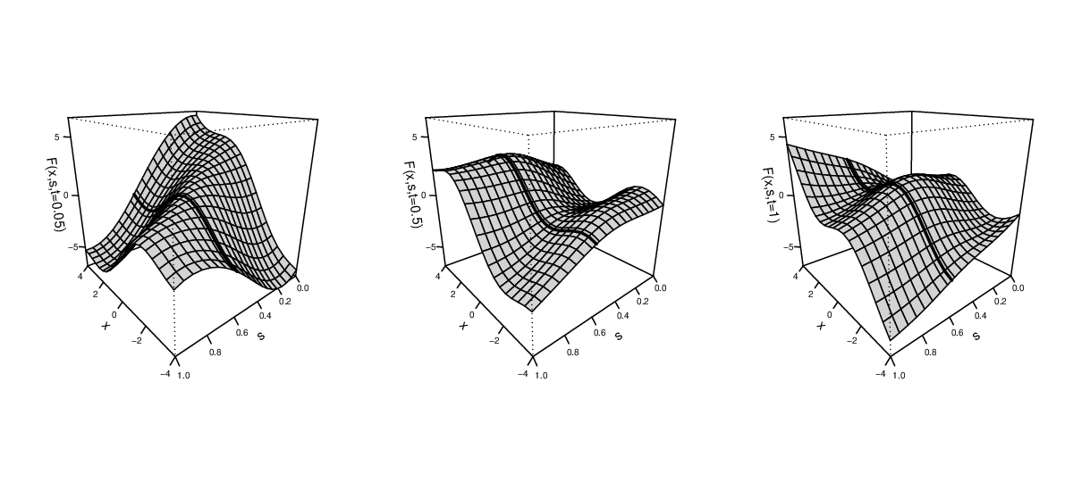
We investigate the finite sample performance of our method through simulations. We generate samples from model (1) with the true functional covariate given by where and vary independently across subjects, specifically, for . Also, the covariate is observed with noise, where the are independent . For each sample we generate training sets of size and and a test set of size 50; also . The training sets include two different scenarios for the sampling of and . (i) Dense design - the grids of points and are the same across , and , and are defined as the set of 81 and 101 equidistant points in [0, 1] respectively. (ii) Sparse design - for each the number of observation points and ; the time-points and are randomly sampled without replacement from a set of 81 and 101 equidistant points in [0, 1] respectively.
The test set is generated using the set of 81 and 101 equispaced points in [0, 1] for and , respectively. We denote realizations of the error process by and generate them using four different covariance structures; these cases are denoted by , where assumes a simple independent error structure, and other cases have correlated structure with increasing complexity and are described in Section C of the Supplementary Material. We consider three forms of true function : linear function , simple nonlinear function , and complex nonlinear function . Figure 1 shows the true surface of along with and at fixed points , and . The thick solid line is evaluated at fixed values for and so that only varies; the nonlinearity of this curve indicates a departure from a functional linear model where would be linear in . The remaining details about the simulation are in Supplementary Material, Section C.
The performance of AFF-PC was assessed in terms of in-sample and out-of-sample predictive accuracy, as measured by the root mean squared prediction error (RMSPE), average computation time, and coverage probabilities of prediction intervals. The in-sample and out-of-sample root mean squared prediction error (RMSPE) are denoted by and , respectively. We define the in-sample RMSPE by
where and its estimate are from the Monte Carlo simulation. The out-of-sample RMSPE, denoted by RMSPE, is defined similarly. For each prediction we calculate the average coverage probability of the pointwise prediction intervals.
5.1 Competitive Methods
We compare our method to three other approaches: the functional linear model, the functional additive model of Müller and Yao (2008), which we label FAM, and the B-spline based estimation of Scheipl et al. (2015), AFF-S. Details about the selection of the tuning parameters for our approach and the competitive approaches are in Section C of the Supplementary Material. We assess the prediction accuracy of the proposed approach and three competitive alternatives and compare their computational efficiency. Due to the high computational cost of the functional additive model and AFF-S, we restrict our comparisons with these methods to the case where and the error process () is either or as described in Section C of the Supplementary Material. For the functional linear model, we consider a model defined by . Implementation details of our method and the three other approaches are summarized in the Supplementary Material, Section C.3.
5.2 Simulation Results
5.2.1 Prediction Performance
| (1) | (2) | (1) | (2) | (1) | (2) | (1) | (2) | (1) | (2) | (1) | (2) | (1) | (2) | (1) | (2) | |||||||||||||||||
| n | , dense design | , sparse design | ||||||||||||||||||||||||||||||
| 50 | 0.00 | -0.71 | 0.22 | -1.41 | 0.27 | -0.67 | 0.27 | -2.04 | -0.29 | -5.81 | 0.00 | -6.37 | 0.00 | -4.37 | 0.00 | -5.66 | ||||||||||||||||
| 100 | 0.31 | -0.88 | 0.00 | -0.87 | 0.00 | -0.84 | 0.00 | -0.85 | -0.30 | -3.88 | 0.00 | -4.58 | -0.27 | -3.79 | -0.27 | -3.79 | ||||||||||||||||
| 300 | 0.00 | 0.00 | 0.00 | -1.06 | 0.00 | 0.00 | 0 .00 | 0.00 | 0.00 | -1.98 | -0.23 | -2.94 | 0.00 | -1.96 | -0.27 | -1.96 | ||||||||||||||||
| n | , dense design | , sparse design | ||||||||||||||||||||||||||||||
| 50 | 5.20 | 31.97 | 3.38 | 38.51 | 6.74 | 44.81 | 5.93 | 35.95 | 5.47 | 29.80 | 3.15 | 26.80 | 5.91 | 32.91 | 4.84 | 22.29 | ||||||||||||||||
| 100 | 6.36 | 41.84 | 4.04 | 50.00 | 6.95 | 56.55 | 6.67 | 50.34 | 6.65 | 41.67 | 3.59 | 37.93 | 6.13 | 45.58 | 5.59 | 36.05 | ||||||||||||||||
| 300 | 6.97 | 55.80 | 4.26 | 63.04 | 6.91 | 66.19 | 6.65 | 64.75 | 7.53 | 55.40 | 4.03 | 52.52 | 6.63 | 60.00 | 6.10 | 53.57 | ||||||||||||||||
| n | , dense design | , sparse design | ||||||||||||||||||||||||||||||
| 50 | 34.38 | 58.77 | 24.32 | 58.21 | 30.61 | 56.21 | 30.61 | 55.34 | 31.71 | 52.37 | 22.69 | 51.18 | 28.60 | 50.86 | 28.60 | 50.21 | ||||||||||||||||
| 100 | 36.36 | 65.30 | 25.59 | 64.61 | 31.99 | 63.33 | 31.99 | 62.64 | 34.16 | 59.68 | 24.38 | 58.43 | 30.07 | 58.20 | 30.07 | 57.75 | ||||||||||||||||
| 300 | 37.57 | 70.19 | 26.38 | 69.95 | 32.60 | 69.32 | 32.60 | 68.85 | 35.88 | 67.29 | 25.33 | 66.59 | 31.41 | 66.67 | 31.23 | 66.43 | ||||||||||||||||
The comparison with the functional linear model is summarized in Table 1. For in-sample prediction accuracy, we report the relative percent gain in prediction with respect to functional linear model by computing where and are the in-sample prediction errors obtained by fitting the AFF-PC and functional linear model, respectively. Relative improvement for out-of-sample prediction is measured similarly. Thus, values closer to indicate similar prediction performance between the two models, while larger positive values are indicative of AFF-PC having greater prediction accuracy than the functional linear model. The top part of Table 1 contains the case when the underlying true model is linear in ; the true relationship is described by . Both AFF-PC and the functional linear model, provide relatively similar in-sample and out-of-sample prediction performance in all scenarios. The number of subjects, the sampling design of the grid points, and the error structure slightly affect the numerical results. The results confirm that when the true relationship is linear, then AFF-PC has similar prediction performance as the functional linear model, although there are few cases, especially for sparse designs and smaller sample sizes, where AFF-PC is slightly worse at out-of-sample prediction. The middle and bottom parts of the table have results for the case where the true model in nonlinear; the true relationship is described by (simple nonlinear, middle) and (complex nonlinear, bottom).
The results confirm that if the true model is nonlinear, then AFF-PC shows a dramatic improvement in prediction accuracy over the functional linear model.Depending on the complexity of the mean model, AFF-PC improves prediction accuracy compared to the functional linear model by over . This improvement increases as the sample size gets larger.
Next, we compare AFF-PC to the AFF-S estimator (Scheipl et al., 2015), which uses B-splines rather than an eigenbasis to represent the trajectories. The results are presented in Table 2. Comparing the columns labeled (1) and (2) in the two panels, we observe that the two estimators have similar accuracy, with accuracy varying slightly with the complexity of the relationship. Column labeled (3) shows the average computation time (in seconds), indicating an order of magnitude improvement by AFF-PC over AFF-S. The models were run on a 2.3GHz AMD Opteron Processor.
Table 2 also compares AFF-PC and FAM. As the model complexity increases, the out-of-sample prediction accuracy of AFF-PC increases compared to FAM. Also, FAM takes much more computation time than AFF-PC, especially when the grid points are sparsely sampled. Computation time is less affected by the error covariance structure than is prediction accuracy.
| dense design | sparse design | ||||||||||||||||||
|---|---|---|---|---|---|---|---|---|---|---|---|---|---|---|---|---|---|---|---|
| method | (1) | (2) | (3) | (1) | (2) | (3) | (1) | (2) | (3) | (1) | (2) | (3) | |||||||
| FAM | 0.45 | 0.17 | 94.0 | 0.37 | 0.18 | 92.9 | 0.45 | 0.21 | 687.9 | 0.38 | 0.21 | 920.5 | |||||||
| AFF-S | 0.44 | 0.15 | 99.4 | 0.36 | 0.21 | 82.3 | 0.45 | 0.16 | 43.0 | 0.37 | 0.19 | 38.7 | |||||||
| AFF-PC | 0.44 | 0.14 | 10.2 | 0.37 | 0.15 | 8.7 | 0.45 | 0.17 | 10.2 | 0.38 | 0.17 | 8.9 | |||||||
| FAM | 0.43 | 0.12 | 93.9 | 0.36 | 0.13 | 93.4 | 0.44 | 0.17 | 564.2 | 0.36 | 0.17 | 697.7 | |||||||
| AFF-S | 0.43 | 0.06 | 143.5 | 0.34 | 0.12 | 116.4 | 0.42 | 0.08 | 39.0 | 0.34 | 0.10 | 37.5 | |||||||
| AFF-PC | 0.43 | 0.09 | 6.1 | 0.35 | 0.10 | 7.8 | 0.43 | 0.11 | 7.1 | 0.35 | 0.12 | 9.9 | |||||||
| FAM | 0.48 | 0.28 | 94.4 | 0.41 | 0.29 | 92.7 | 0.49 | 0.32 | 687.2 | 0.42 | 0.33 | 656.3 | |||||||
| AFF-S | 0.45 | 0.21 | 130.3 | 0.37 | 0.27 | 124.1 | 0.45 | 0.23 | 50.6 | 0.38 | 0.26 | 31.0 | |||||||
| AFF-PC | 0.45 | 0.19 | 10.5 | 0.37 | 0.21 | 10.1 | 0.46 | 0.23 | 9.7 | 0.39 | 0.23 | 9.9 | |||||||
In summary, AFF-PC better captures complex nonlinear relationships than the functional linear model, and yet AFF-PC performs as well as the functional linear model when the latter is true. The B-spline based estimator, AFF-S, and AFF-PC have similar prediction performance, while AFF-S and FAM are much slower than AFF-PC.
5.2.2 Performance of the Prediction Intervals
Next, we assess coverage accuracy of the pointwise prediction intervals. These intervals are approximated using the method described in Section 3 with 100 bootstrap samples per simulated data set. Table 3 reports the average coverage probability for both the dense and sparse design at nominal levels of 85%, 90%, and 95%. When the sample size is small (e.g., ), the prediction intervals are conservative, providing greater coverage probabilities than the nominal values. However, the coverage probabilities approach the nominal levels as the sample size increases. The complexity of the true function affects the coverage performance slightly. If the true function is complex, e.g., , the coverage probability converges more slowly to the nominal levels as increases compared to when the true function is simple, e.g., . The number of subjects, the sampling design of the grid points, and the error covariance structure also affect the coverage performance slightly.
Remark.
Section D.1 of the Supplementary Material includes additional simulation results corresponding to another level of sparseness, and the results indicate that our approach still maintains prediction accuracy. Section D.2 of the Supplementary Material illustrates numerically that our method is not sensitive to the choice of .
| , dense design | |||||||||||||||||||
|---|---|---|---|---|---|---|---|---|---|---|---|---|---|---|---|---|---|---|---|
| 0.85 | 0.90 | 0.95 | 0.85 | 0.90 | 0.95 | 0.85 | 0.90 | 0.95 | 0.85 | 0.90 | 0.95 | ||||||||
| 50 | 0.904 | 0.942 | 0.976 | 0.883 | 0.926 | 0.966 | 0.880 | 0.926 | 0.967 | 0.883 | 0.925 | 0.965 | |||||||
| 100 | 0.884 | 0.928 | 0.967 | 0.869 | 0.916 | 0.960 | 0.866 | 0.916 | 0.961 | 0.869 | 0.915 | 0.959 | |||||||
| 300 | 0.868 | 0.915 | 0.960 | 0.859 | 0.908 | 0.955 | 0.856 | 0.908 | 0.957 | 0.858 | 0.908 | 0.953 | |||||||
| , sparse design | |||||||||||||||||||
| 50 | 0.910 | 0.946 | 0.977 | 0.882 | 0.926 | 0.965 | 0.888 | 0.930 | 0.969 | 0.887 | 0.928 | 0.967 | |||||||
| 100 | 0.887 | 0.930 | 0.969 | 0.870 | 0.916 | 0.960 | 0.870 | 0.918 | 0.963 | 0.873 | 0.918 | 0.961 | |||||||
| 300 | 0.867 | 0.915 | 0.960 | 0.860 | 0.909 | 0.956 | 0.858 | 0.910 | 0.958 | 0.862 | 0.910 | 0.955 | |||||||
| , dense design | |||||||||||||||||||
| 50 | 0.936 | 0.963 | 0.986 | 0.914 | 0.948 | 0.978 | 0.912 | 0.947 | 0.978 | 0.911 | 0.946 | 0.977 | |||||||
| 100 | 0.913 | 0.949 | 0.979 | 0.895 | 0.935 | 0.970 | 0.895 | 0.935 | 0.972 | 0.893 | 0.933 | 0.970 | |||||||
| 300 | 0.880 | 0.924 | 0.966 | 0.871 | 0.917 | 0.961 | 0.870 | 0.916 | 0.962 | 0.869 | 0.914 | 0.959 | |||||||
| , sparse design | |||||||||||||||||||
| 50 | 0.949 | 0.971 | 0.989 | 0.913 | 0.947 | 0.977 | 0.931 | 0.958 | 0.982 | 0.932 | 0.959 | 0.983 | |||||||
| 100 | 0.923 | 0.954 | 0.982 | 0.895 | 0.936 | 0.971 | 0.903 | 0.941 | 0.975 | 0.903 | 0.940 | 0.974 | |||||||
| 300 | 0.889 | 0.931 | 0.970 | 0.877 | 0.922 | 0.964 | 0.879 | 0.923 | 0.966 | 0.878 | 0.921 | 0.963 | |||||||
6 Capital Bike Share Data
We now turn to the capital bike share study (Fanaee-T and Gama, 2013). The data were collected from the Capital Bike Share system in Washington, D.C., which offers bike rental services on an hourly basis. In recent years, there has been an increased demand for bicycle rentals; renting is viewed as an attractive alternative to owing bicycles. Thus, ensuring a sufficient bike supply represents an important factor for a successful business in this area. In this paper we try to gain a better understanding of the customers’ rental behavior during the a weekend day in relation to the weather condition for that day. We are interested in casual rentals, which are rentals to cyclists without membership in the Capital Bike Share program. The counts of casual bike rentals are recorded at every hour of the day, during the period from January 1, 2011 to December 31, 2012, for a total of 105 weeks. Also collected are weather information such as temperature (∘C) and humidity on an hourly basis.

Bike rentals have different dynamics on weekends compared to weekends. We restrict our study to Saturday rentals, when there is a particular high demand for casual bike rentals. Our focus is on how Saturday rentals relate to the temperature, while accounting for humidity. Understanding the nature of this association could help one predict the casual rental demand based on the weather forecast available on the previous day. Figure 2 shows the counts of casual bike rentals (left panel) and hourly temperature (right panel) on Saturdays; each curve corresponds to a particular week. The solid, dotted, and dashed lines are the observations for three different Saturdays. On weekends, many renters can be flexible about when during the day to rent, so it is assumed that the entire temperature curve affects the number of casual bikes rental at any time on Saturday. To remove skewness, we log-transform the response data, , before we proceed with our analysis.
Let be the number of casual bikes rented recorded, on the log-scale, for the Saturday at the hour of the day; also let denote the true temperature for the Saturday at the hour of the day and let be the average humidity for the corresponding Saturday. We consider the general additive function-on-function regression AFF-PC model
| (11) |
where is the marginal mean of the response, is an unknown trivariate function capturing the effect of the daily temperature and is a smooth univariate function that quantifies the time-varying effect of the average humidity.
The temperature and the counts of bike rentals have a small amount of missingness. Therefore, we smoothed the temperature profiles using functional principal component analysis before applying the center/scaling transformation. We assessed both in-sample and out-of-sample prediction accuracy by splitting the data into training and test sets of size 89 and 16, respectively. To model the function , we used cubic B-splines for the - and -directions and selected , the number of eigenfunctions for modeling in the direction, by fixing the percentage of explained variance to ; this resulted in . These choices for the tuning parameters are supported by additional sensitivity analysis included in Section E.2 of the Supplementary Material. We also used to model the marginal mean function and the smooth effect of average humidity , and , where and are the unknown basis coefficients. Such a representation allows us to use also to control the smoothness of the fitted coefficient function, . Parameter estimation was done as described in Section 2.2 with minor modifications due to the additional covariate, average humidity. Briefly, to estimate the unknown parameters, , and , we constructed , , and and then minimized the penalized criterion (5) using and in place of and , respectively.
 |
 |
|
|---|---|---|
 |
 |
 |
Figure 3 shows the estimated parameter functions: the top two plots illustrate the estimated intercept function and . On average the number of casual bike rentals decreases until 5AM ( on the plot) and then increases steadily peaking at about 3:00PM (). As expected, humidity is negatively associated with the bike rentals; the effect seems to be largest at 3:00PM. The bottom panels show the contour plots of the function for three values of , (midnight), (noon) and (evening, 8PM); the values of have a standardized interpretation. For example, is interpreted as one standard deviation away from the mean temperature profile.
As mentioned in Section 2.1, the functional linear model is the special case of (1) where , which implies that does not depend on . The nonlinearity of in can be noted in all these plots but in particular in the middle bottom panel (). Consider the case when ; simple calculations yield that the partial derivative of with respect to at is different from the one for , and thus that is not linear in .
Table 4 compares AFF-PC, AFF-S, and the functional linear model. AFF-PC results in better prediction performance than functional linear model for both in-sample and out-of sample. As expected, AFF-PC and AFF-S have similar accuracy but AFF-PC is much faster than AFF-S.
| log-transformed data | original data | |||||||||||||||
| Method | (, , ) | (1) | (2) | (1) | (2) | (3) | ||||||||||
| FLM | (NA, 7,7) | 0.740 | 0.606 | 62.079 | 43.603 | 2.12 | ||||||||||
| AFF-S | (7,7,7) | 0.637 | 0.494 | 37.275 | 28.826 | 25.36 | ||||||||||
| AFF-PC | (7,7, ) | 0.635 | 0.493 | 38.184 | 31.715 | 1.97 | ||||||||||
Furthermore, we can construct bootstrap-based prediction intervals for the predicted trajectories in the test set, by slightly modifying the bootstrap procedure included in Section 3.2. For completeness, the algorithm is provided in the Supplementary Material, Section E.3. Figure 4 illustrates the 95% prediction bands constructed for three different Saturdays in the test set. Finally, we assessed the coverage probability of the prediction intervals. AFF-PC tended to produce conservative prediction intervals. For example, using bootstrap replications, the actual coverage probability of the prediction intervals was with a standard error of .

7 Discussion
This article considered additive regression models for functional responses and functional covariates. These models are a generalization of the functional linear model and allow for a nonlinear relationship between the response and the covariate. We proposed a novel estimation technique, AFF-PC, that is computationally very fast. We developed prediction inference for a future functional outcome when the functional covariate is known. As illustrated by the bike share study, AFF-PC can accommodate additional scalar or vector covariates. Furthermore, AFF-PC can easily be extended to accommodate multiple functional covariates. We showed through numerical study that when the true model is linear, AFF-PC’s performance is very close to that of the functional linear model, but if the true model is nonlinear, AFF-PC can yield considerably improved prediction performance. The capital bike share data is available at: https://archive.ics.uci.edu/ml/datasets/Bike+Sharing+Dataset. The R code used in the simulation is available at: http://www4.stat.ncsu.edu/~staicu/Code/affpccode.zip.
Supplementary Material
- Supplementary Material:
-
Additional descriptions for methodology extensions, simulation setup, and simulation results are provided. (pdf file)
- R code:
-
The R code developed for the simulation. (zip file)
Acknowledgements
Staicu’s research was funded by National Science Foundation grant DMS 1454942 and National Institute of Health grants R01 NS085211 and R01 MH086633. Maity’s research was partially funded by National Institutes of Health award R00 ES017744 and a North Carolina State University Faculty Research and Professional Development award. Carroll’s research was supported by a grant from the National Cancer Institute (U01-CA057030). The research of Ruppert was partially supported by National Science Foundation grant AST 1312903 and by a grant from the National Cancer Institute (U01-CA057030).
References
- Aston et al. (2010) Aston, J. A. D., J. M. Chiou, and J. P. Evans (2010). Linguistic pitch analysis using functional principal component mixed effect models. Journal of the Royal Statistical Society, Series C 59, 297–317.
- Benko et al. (2009) Benko, M., W. Härdle, A. Kneip, et al. (2009). Common functional principal components. The Annals of Statistics 37(1), 1–34.
- Cuevas et al. (2006) Cuevas, A., M. Febrero, and R. Fraiman (2006). On the use of the bootstrap for estimating functions with functional data. Computational statistics & data analysis 51(2), 1063–1074.
- Cuevas and Fraiman (2004) Cuevas, A. and R. Fraiman (2004). On the bootstrap methodology for functional data. In COMPSTAT 2004 Proceedings in Computational Statistics, pp. 127–135. Springer.
- Di et al. (2009) Di, C.-Z., C. M. Crainiceanu, B. Caffo, and N. M. Punjabi (2009). Multilevel functional principal component analysis. Annals of Applied Statistics 3, 458–488.
- Fanaee-T and Gama (2013) Fanaee-T, H. and J. Gama (2013). Event labeling combining ensemble detectors and background knowledge. Progress in Artificial Intelligence, 1–15.
- Ferraty et al. (2010) Ferraty, F., I. Van Keilegom, and P. Vieu (2010). On the validity of the bootstrap in non-parametric functional regression. Scandinavian Journal of Statistics 37(2), 286–306.
- Ferraty et al. (2012) Ferraty, F., I. Van Keilegom, and P. Vieu (2012). Regression when both response and predictor are functions. Journal of Multivariate Analysis 109, 10–28.
- Goldsmith et al. (2013) Goldsmith, J., S. Greven, and C. Crainiceanu (2013). Corrected confidence bands for functional data using principal components. Biometrics 69, 41–51.
- Hastie and Tibshirani (1986) Hastie, T. and R. Tibshirani (1986). Generalized additive models. Statistical Science 1, 297–310.
- Huang et al. (2015) Huang, L., F. Scheipl, J. Goldsmith, J. Gellar, J. Harezlak, M. W. McLean, B. Swihart, L. Xiao, C. Crainiceanu, and P. Reiss (2015). refund: Regression with Functional Data. R package version 0.1-13.
- Jiang and Wang (2010) Jiang, C.-R. and J.-L. Wang (2010). Covariate adjusted functional principal components analysis for longitudinal data. Annals of Statistics 38, 1194–1226.
- Kim et al. (2016) Kim, J., A. Maity, and A. M. Staicu (2016). General functional concurrent model. Unpublished manuscript (under review).
- Malfait and Ramsay (2003) Malfait, N. and J. O. Ramsay (2003). The historical functional linear model. The Canadian Journal of Statistics 31, 115–128.
- Marx and Eilers (2005) Marx, B. D. and P. H. C. Eilers (2005). Multivariate penalized signal regression. Technometrics 47, 13–22.
- McLean et al. (2014) McLean, M. W., G. Hooker, A. M. Staicu, F. Scheipl, and D. Ruppert (2014). Functional generalized additive models. Journal of Computational and Graphical Statistics 23, 249–269.
- Müller et al. (2013) Müller, H.-G., Y. Wu, and F. Yao (2013). Continuously additive models for nonlinear functional regression. Biometrika 103, 607–622.
- Müller and Yao (2008) Müller, H.-G. and F. Yao (2008). Functional additive models. Journal of the American Statistical Association 103, 1534–1544.
- Paparoditis and Sapatinas (2016) Paparoditis, E. and T. Sapatinas (2016). Bootstrap-based testing of equality of mean functions or equality of covariance operators for functional data. Biometrika 103(3), 727–733.
- Park and Staicu (2015) Park, S. Y. and A. M. Staicu (2015). Longitudinal functional data analysis. Stat 4, 212–226.
- Politis and Romano (1994) Politis, D. N. and J. P. Romano (1994). Limit theorems for weakly dependent hilbert space valued random variables with application to the stationary bootstrap. Statistica Sinica, 461–476.
- Pomann et al. (2015) Pomann, G.-M., A.-M. Staicu, and S. Ghosh (2015). Two sample hypothesis testing for functional data. Unpublished manuscript (submitted).
- Ramsay and Silverman (2005) Ramsay, J. O. and B. W. Silverman (2005). Functional Data Analysis (2nd ed.). New York, Springer.
- Redd (2012) Redd, A. (2012). A comment on the orthogonalization of b-spline basis functions and their derivatives. Statistics and Computing 22, 251–257.
- Ruppert et al. (2003) Ruppert, D., M. P. Wand, and R. J. Carroll (2003). Semiparametric Regression. Cambridge, New York: Cambridge University Press.
- Scheipl et al. (2015) Scheipl, F., A.-M. Staicu, and S. Greven (2015). Functional additive mixed models. Journal of Computational and Graphical Statistics 24, 477–501.
- Sentürk and Nguyen (2011) Sentürk, D. and D. V. Nguyen (2011). Varying coefficient models for sparse noise-contaminated longitudinal data. Statistica Sinica 21, 1831–1856.
- Wood (2006) Wood, S. N. (2006). Generalized Additive Models: An Introduction with R. Boca Raton, Florida: Chapman and Hall/CRC.
- Wu et al. (2010) Wu, Y., J. Fan, and H.-G. Müller (2010). Varying-coefficient functional linear regression. Bernoulli 16, 730–758.
- Yao et al. (2005a) Yao, F., H.-G. Müller, and J.-L. Wang (2005a). Functional data analysis for sparse longitudinal data. Journal of the American Statistical Association 100, 577–590.
- Yao et al. (2005b) Yao, F., H.-G. Müller, and J.-L. Wang (2005b). Functional linear regression analysis for longitudinal data. Annals of Statistics 33, 2873–2903.
- Zhang and Chen (2007) Zhang, J.-T. and J. Chen (2007). Statistical inference for functional data. Annals of Statistics 35, 1052–1079.