Non-adiabatic bulk-surface oscillations in driven topological insulators

The simplest model of a TI surface state is a single Dirac cone with Hamiltonian [9]

for a surface perpendicular to $\hat{z}$. The Pauli matrices often correspond to physical spin $(S^{x},S^{y})=(\sigma^{y},-\sigma^{x})/2$ which is locked perpendicular to the momentum $\boldsymbol{\mathbf{k}}_{\parallel}$ via Rashba spin-orbit coupling [56, 57, 58], though more generally $\sigma$ could denote spin/orbital indices. Our units are set by velocity $v=1$, as well as $\hbar=1$ throughout the paper. Consider driving this Hamiltonian by a laser perpendicular to the surface, with electric field $\boldsymbol{\mathbf{E}}=E_{x}\cos(\Omega t+\varphi_{x})\hat{x}+E_{y}\sin(\Omega t+\varphi_{y})\hat{y}$ of constant amplitude. This drive allows arbitrary polarization, but we will focus on the case of linearly $y$-polarized light and phase $\varphi_{y}=0$. Coupling this periodic drive to the surface states is achieved by the minimal substitution $\boldsymbol{\mathbf{k}}_{\parallel}\to\boldsymbol{\mathbf{k}}_{\parallel}-e\boldsymbol{\mathbf{A}}$, where we pick the gauge $\boldsymbol{\mathbf{E}}=-\partial\boldsymbol{\mathbf{A}}/\partial t$. Then the Hamiltonian becomes time-dependent:

We first consider the case of constant drive amplitude, $E_{y}=\Omega A_{y}$, but later we will return to the case where this amplitude in turn varies slowly as in the case of a pulsed laser (cf. Fig. 2b). Note that we are assuming the drive is uniform over the entire sample such that the in-plane momentum $\boldsymbol{\mathbf{k}}_{\parallel}$ remains a conserved quantity even in the presence of the drive.

To understand the relevance of the bulk, we want to start by constructing a simple tight-binding model of a three-dimensional topological insulator. We consider one of the simplest such bulk models [54], namely the lattice regularization of $(\boldsymbol{\mathbf{k}}\cdot\boldsymbol{\mathbf{\sigma}})\tau^{z}+m\tau^{x}$:

where $\sigma$ and $\tau$ are two sets of Pauli matrices corresponding to, e.g., spin and orbital degrees of freedom. We again assume that the electric field couples via the minimal substitution, but now with the caveat that the electric field strength decays into the bulk with length scale $\xi$, as in Fig. 1. Choosing the surface of interest to again be perpendicular to $\hat{z}$, $\boldsymbol{\mathbf{k}}_{\parallel}=(k_{x},k_{y})$ remain good quantum numbers. For more details of the hopping Hamiltonian in the $z$-direction, please see Appendix A.

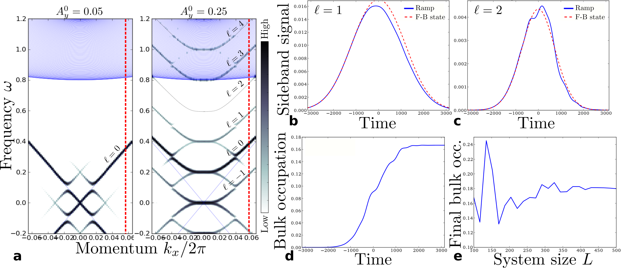
In the absence of drive, this model gives a topological insulator for $-4<m<0$ and a trivial insulator otherwise. In the presence of drive, we can solve this Floquet problem and calculate its Wigner distribution. The results are shown in Fig. 3a. Similar to the simple surface-only model, the surface states are strongly dressed by the drive, although details of the signal depend heavily on microscopic details of the model. At strong driving strength $A_{y}=0.25$, this “Floquet equilibrium” (i.e., constant drive amplitude) data already shows how coupling to the bulk changes the story, resulting in $\ell=3$ and $4$ sidebands that are stronger than $\ell=2$ due to resonant surface-bulk hybridization. In the next section we will see that this surface-bulk coupling has a strong effect when we consider a pulsed drive.

We now simulate the coupled bulk-surface model of a TI under such pumped drive. We start deep in the past with the drive turned off and the chemical potential set such that all bulk valence band and surface states are occupied. ²² 2 In practice, we actually just compute time evolution of the surface states on the upper surface as the remaining states do not affect the signal. We have verified that occupying the valence bands does not change our results. Then the exact dynamics are simulated and the Wigner distribution $f(\omega,t_{\mathrm{av}})$ computed. This function is strongly peaked in $\omega$ and highly oscillatory in $t_{\mathrm{av}}$ so we smooth out the results by convolving $f$ by a Gaussian of width $\tau_{\mathrm{pr}}$ in both the frequency and time direction:

We refer to the result as the signal and/or intensity at frequency $\omega$ and time $t_{\mathrm{av}}$, which will be justified in Sec. II.3 by showing its connection to ARPES. If the “probe width” $\tau_{\mathrm{pr}}$ is much greater than the drive frequency, this convolution has the additional advantage of averaging over the drive phase, such that $f$ may be replaced by $\overline{f}$ in Eq. 9.

One striking difference between the equilibrium and non-equilibrium case is that, even after the drive has been turned off, population remains in the bulk conduction states, as seen in Fig.  3d. This phenomenon is specific to the coupled bulk/surface model, and we do not see it in the simpler Dirac cone model of Sec. I.1. Decay of excited surface states into the bulk has been anticipated in the presence of phonons [40], but note that this decay mechanism does not exist in our model. Therefore, the population transferred to the bulk may only come from coherent non-adiabatic processes.

In addition to tunneling into the bulk, we see coherent oscillations in the Wigner distribution of the surface states. This is shown in Fig. 3b and c, where the signal in the $\ell$th sideband is given by weight in the $\ell$th peak at fixed $k_{x}$ and $t_{\mathrm{av}}$ normalized by the sum over all peaks. Together, these results suggest that we are seeing coherent oscillations of the population between the surface and the bulk states. We have varied the microscopic parameters over a wide range of values and found that the existence of these oscillations are remarkably robust, always appearing in tandem with an irreversible “leaking” into the bulk. We now seek to understand this in terms the physics of Floquet resonances.

Resonances have long been known to play a major role in Floquet systems [70, 71, 72, 73]. Mathematically, they come from the fact that the drive introduces a new energy scale $\Omega$ such that energies are only defined modulo $\Omega$. For a many-body system of linear size $L$ in $d$ dimensions, the bare spectrum is extensive, scaling as $L^{d}$. However, Hone et al. [73] argued that folding by $\Omega$ in the thermodynamic limit leads to a denser and denser set of quasi-energy levels as the system size is increased. This in turn leads to a dense set of weakly-avoided crossings such that even simple ideas like tracking a single quasi-energy level to achieve an adiabatic limit becomes ill-defined. Thus the weakly-avoided crossings, which we call Floquet resonances, lead to a fundamental absence of adiabaticity in Floquet systems. Furthermore, they have been suggested to lead to heating effects [74] and the breakdown of high-frequency expansions [75], which are two of the most important and active topics in the field of Floquet engineering.

As seen in Fig. 3a, Floquet resonances between the surface and the bulk states inevitably occur in systems such as ours, where the driving frequency $\Omega$ is less than the bandwidth. However, there are a number of subtleties that we must consider in comparing this to the Hone et al. result. Most notably, they were considering coupling between bulk states due to the drive, whereas here we are interested in coupling between the bulk and the surface state. Since the drive primarily couples to the surface states and only weakly to the bulk, one naive guess would be that the matrix elements between these states would scale as the spatial overlaps between them, $\xi/L$, vanishing in the thermodynamic limit. This indeed seems to be the case, but one must counterbalance it against the fact that the (one-dimensional) density of states at fixed $\boldsymbol{\mathbf{k}}_{\parallel}$ scales as $L$. Thus these two effects conspire to create an order-1 gap in the quasi-energy spectrum which depends sensitively on various microscopic properties. Therefore, we expect that the strength will differ significantly from model to model, e.g., between our simple model TI and a real material. Nevertheless, the existence of order 1 Floquet resonances should be robust by the above argument, and thus the phenomena we describe are completely generic.

As seen in Fig. 4a, Floquet resonances lead to a series of anti-crossings between quasienergies of the bulk and surface states. As expected, the quasienergy of the surface state depends strongly on driving amplitude, while the bulk states are nearly independent of the drive. We also confirm that as $L$ increases the number of anti-crossings increases as well, while the strength (i.e., the gap) of the anti-crossings decreases. This situation, where a single dispersing level passes through many parallel non-dispersing ones is known in the non-Floquet case as the Demkov-Osherov (D-O) model [76, 77, 78], and is an analytically tractable many-level generalization of the Landau-Zener (L-Z) model [79, 80]. The scattering matrix of the D-O model in the long-time limit is remarkable because interference between the various avoided crossings is absent. Thus, the D-O scattering problem reduces to $N_{c}$ independent L-Z transitions, where $N_{c}$ is the number of bulk levels that the dispersing level surface state crosses. In our case, $N_{c}\sim L$ at fixed $\boldsymbol{\mathbf{k}}_{\parallel}$ because we effectively have a one-dimensional problem.

For slow ramps, one expects that the dynamics of a Floquet system will be dominated by resonant effects, which are captured within the appropriately-folded effective Hamiltonian $H_{F}$. Therefore, we should be able to able to treat the Floquet D-O model identically to the undriven case. Assume the surface state is ramped through $N_{c}$ bulk states during the first half of the pump pulse by increasing $A_{y}$ from $0$ to $A_{y}^{0}$ such that the surface state quasienergy increases at a constant velocity $v=d\epsilon/dt$. As each crossing may be treated independently, the final probability to be in the surface state is just the product of the individual probabilities:

This looks exactly like the L-Z problem for a single avoided crossing with matrix element $\Delta_{\mathrm{eff}}=\sqrt{\sum_{j}\Delta_{j}^{2}}$, as illustrated in Fig. 4b. In the thermodynamic limit, we expect these gaps to scale as $\Delta_{j}\sim\Delta_{0}/\sqrt{L}$ from the scaling of the overlap of bulk and surface eigenstates. Thus the dynamics of our model is expected to have a consistent $L\to\infty$ limit, which is confirmed numerically in Fig. 3e. In addition to the final bulk occupation, this effective gap also controls the time scale of the oscillations in the surface state sidebands. Thus we see that both the incoherent transition to bulk states and coherent bulk-surface oscillations survive in the thermodynamic limit with dynamics set by the same emergent energy scale.

In addition to giving a physical picture for both the surface-bulk oscillations and the non-adiabatic tunneling of electrons into the bulk, the Demkov-Osherov model provides a handle for understanding how these should change with the various parameters, such as the experimentally-controllable $\tau_{\mathrm{pump}}$. One important upshot is the meaning of “adiabaticity” reversed from what we expect in the absence of resonances. Normally one expects the adiabatic limit to correspond to slow ramping, such that the system tracks the instantaneous Floquet eigenstate. However, it is clear for the resonant case that ramping the field too slowly will cause the entire population to transfer into the bulk. Therefore, to “adiabatically” track the surface state, one must instead use a fast ramp, though still sufficiently slow to prevent direct non-resonant excitations to the bulk.[73, 81, 75] More explicitly, we expect that the population remaining in the surface state at the end of the ramp should scale as $p_{ss}^{f}=e^{-4\pi\Delta_{\mathrm{eff}}^{2}/v}\sim e^{-(4\pi\Delta_{\mathrm{eff}}^{2}/\Delta\epsilon)\tau_{\mathrm{pump}}}\equiv e^{-2\Gamma\tau_{\mathrm{pump}}}$, where the additional factor of two compared to Eq. 10 comes from ramping up to $A_{y}^{0}$ then back down to $0$. This dependence is consistent with the data, as shown in Fig. 5d. By a similar token, increasing $\tau_{\mathrm{pump}}$ increases the size of the resonant bulk-surface oscillations, as seen in Fig. 5a-c. It is interesting to note that a similar “ghost” surface state has been found in static models of topological materials coupled to a trivial bulk [82, 83], which may be solved by modeling it with the well-known Fano model [84]. Ours is the natural Floquet generalization of these ideas, leading to fundamentally non-equilibrium phenomena such as coherent bulk-surface oscillations and Floquet resonances. Further discussion of the Demkov-Osherov model and its application to surface-driven systems may be found in Appendix B.

Before concluding this section, we note that our results our directly applicable to time-resolved ARPES experiments. Time-resolved pump-probe ARPES works by driving the system at frequency $\Omega$ with a Gaussian envelope (the pump) which excites that electrons in the sample but does not cause it to photoemit. Then, at variable times during the pump, a weak probe pulse at much higher frequency and much shorter width $\tau_{\mathrm{pr}}$ is shone on the sample, which excites the driven electrons above the work function of the material. These electrons are then (photo)emitted by the sample and subsequently detected. By measuring the energy and momenta of the photoemitted electrons, the detector is able to map out the material’s band structure during the probe pulse, including any non-equilibrium effects given by the pump.

Theoretically, the time-resolved ARPES signal for an arbitrary driven Hamiltonian $H(t)$ is given by [85, 66]

if one ignores that matrix elements between the electrons in the material and the photoemitted states. A brief discussion of the effect of non-trivial matrix elements is found in Appendix C. If one uses a Gaussian probe, $s_{\mathrm{pr}}(t)=\exp(-t^{2}/2\tau_{\mathrm{pr}}^{2})$, then Eq. 11 reduces to Eq. 9. Thus, all of the results we have shown so far can be simply interpreted as the signal of a time-resolved ARPES experiment with a Gaussian pump and probe, and our results serve as an important experimentally-accessible signature of this novel bulk-surface coupling.

Adiabatic perturbation theory (APT) is a technique to derive leading corrections to the adiabatic limit for a system with a parameter $\lambda$ that is ramped slowly with time [86, 87, 88, 89, 90]. Floquet APT (FAPT) extends this idea to a periodically driven system, which is relevant for our setup with parameter $\lambda=A_{y}$ ramped slowly during the pump pulse. Consider as before the case where the system starts with drive turned off in the single particle eigenstate $|0\rangle$ of undriven Hamiltonian $H(\lambda(t_{0}))$. Turning on the drive slowly, the full time evolution is captured in the wave function $|\psi(t)\rangle$. We can approximately solve the problem by doing a unitary rotation to the moving frame: $|\tilde{\psi}\rangle=V^{\dagger}|\psi\rangle$, where $V(\lambda(t),t)=P(\lambda,t)U_{d}(\lambda)$ is a unitary that maps the Floquet eigenstates $|n_{F}(\lambda,t)\rangle$ (see Eq. 6) to a fixed basis $|e_{n}\rangle$. In particular if we were to imagine turning on $\lambda$ infinitely slowly in a gapped Floquet system, then the initial state $|0\rangle$ would just adiabatically track to the Floquet eigenstate $|\psi(t)\rangle=|0_{F}(\lambda,t)\rangle$ and $V^{\dagger}$ would act to map this to a time and $\lambda$-independent state $|\tilde{\psi}\rangle=|e_{0}\rangle$. For a generic time evolution $\lambda(t)$, the effective Hamiltonian in this moving frame is given by

where $H_{F}^{d}$ is a diagonal matrix whose entries correspond to the Floquet quasienenergies and $A_{F}(\lambda,t)=V\tilde{A}_{F}V^{\dagger}$ is the natural Floquet generalization of the Berry connection operator, with matrix elements $\langle m_{F}(\lambda,t)|A_{F}|n_{F}(\lambda,t)\rangle=i\langle m_{F}(\lambda,t)|\partial_{\lambda}n_{F}(\lambda,t)\rangle$. In the adiabatic limit ($\dot{\lambda}\to 0$), off-diagonal elements of the second term in Eq. 12 are unable to cause transitions, which yields the adiabatic loading of the Floquet eigenstates as we just discussed.

Floquet APT consists of solving leading corrections to adiabaticity induced by the second term in Eq. 12. As this term is small due to the slow ramp rate $\dot{\lambda}$, it can be treated perturbatively. In particular, one may note that at fixed $\lambda$, $\tilde{A}_{F}$ is a periodic operator with Fourier series $\tilde{A}_{F}=\sum_{\ell}\tilde{A}_{F}^{(\ell)}e^{i\ell\Omega t}$ and similarly for $V$. Then Eq. 12 yields a Floquet problem which we can approximately solve using static perturbation theory. Expanding the wave function $|\psi(t)\rangle=\sum_{n}c_{n}|n_{F}(\lambda(t),t)\rangle$, the coefficients at leading order in adiabatic perturbation theory are given by [81]

The phase $\Theta_{0}$ that the wave function picks up during the ramp consists of a dynamical and a Berry phase:

This phase is usually neglected in most APT calculations of single-time observables, but is crucial to situations like ARPES where non-equilibrium observables are measured.

One can now use the approximate wave function $|\psi(t)\rangle$ derived above to obtain the Wigner distribution, $f(t_{\mathrm{av}},t_{\mathrm{r}})=\langle\psi(t_{\mathrm{av}}+t_{\mathrm{r}}/2)|\psi(t_{\mathrm{av}}-t_{\mathrm{r}}/2)\rangle$. For this Floquet problem, time enters in two ways: in the periodic part of the Floquet eigenstates, and in the slow time-dependence of $\lambda$. In the spirit of FAPT, we expand this slow dependence about the measurement point $t_{\mathrm{av}}$, $\lambda(t_{\mathrm{av}}\pm t_{\mathrm{r}}/2)=\lambda(t_{\mathrm{av}})\pm t_{\mathrm{r}}\dot{\lambda}(t_{\mathrm{av}})/2+O(\dot{\lambda}^{2})$, and solve for the signal $I$ keeping all terms to order $\dot{\lambda}$. This calculation is done in detail in Appendix D, with the following result:

where all expressions are evaluate at time $t_{\mathrm{pr}}$, the sum is taken for all pairs $(n,\ell^{\prime})\neq(0,\ell)$, and notations are explained in the following paragraph.

The effects of these leading corrections to adiabaticity on the ARPES signal are illustrated in Fig. 6. Both the intensity $I^{(\ell)}_{0}=p_{0\ell}=\langle 0_{F}^{(\ell)}|0_{F}^{(\ell)}\rangle$ and the frequency $\omega_{0}^{(\ell)}=\epsilon_{0}^{F}-\ell\Omega$ of the Floquet sideband $|0_{F}^{(\ell)}\rangle$ defined in Eq. 7 are modified by an amount proportional to the ramp rate $\dot{\lambda}$. The intensity shift $\Delta I^{(\ell)}$ results from virtual excitations of $|0_{F}^{(\ell^{\prime})}\rangle$ to $|n_{F}^{(\ell+\ell^{\prime})}\rangle$, which is a relatively standard prediction of adiabatic perturbation theory. Much more surprising are the frequency shifts, as they turn out to come from Berry phase effects. If we isolate the Berry phase sidebands as $|0_{F}^{(\ell)}\rangle=e^{i\varphi^{(\ell)}(\lambda)}|\tilde{0}_{F}^{(\ell)}(\lambda)\rangle$ such that $|\tilde{0}_{F}^{(\ell)}\rangle$ has vanishing Berry connection, then $\Delta\omega^{(\ell)}$ gives the difference of the Berry connection in sideband $\ell$ from the average Berry connection across all sidebands. This object seems somewhat bizarre if for no other reason than the fact that the Berry connection is not gauge-invariant. However, this difference of Berry connections is gauge invariant and leads to a Berry phase-dependent shift of the frequency of the sidebands.

Interestingly, while we think of adiabatic perturbation theory as primarily holding in the limit of small velocities, the results above actual hold in the limit of large (but not too large) velocities in which resonances can be neglected. Similar to the results found earlier in the resonant limit, these corrections in FAPT will lead to an asymmetry in the intensity signal with respect to time $t=0$, even though the Gaussian pulse is symmetric with respect to $t=0$. Unlike the resonant case, these corrections get smaller as the velocity decreases, or equivalently the pump time $\tau_{\mathrm{pump}}$ increases, and the excitations that they describe are virtual, meaning that no real population will remain in the bulk. Combining this with our previous results, we see that as $\tau_{\mathrm{pump}}$ is increased from zero, we get crossovers between various regimes, which are

1. 1.

   $\tau_{\mathrm{pump}}\ll 1/J,1/\Delta$: Non-universal physics related to microscopic details.

2. 2.

   $1/J,1/\Delta\ll\tau_{\mathrm{pump}}\ll 1/\Delta_{\mathrm{res}}$: Virtual excitations described by Floquet adiabatic perturbation theory.

3. 3.

   $1/\Delta_{\mathrm{res}}\ll\tau_{\mathrm{pump}}$: Real excitations due to surface-bulk resonances.

In the low-frequency weak-drive limit, we expect these regimes to be well separated [48], but whether such a separation of scales occurs in general is an important open question.

References

- [1] K. v. Klitzing, G. Dorda, and M. Pepper, Phys. Rev. Lett. 45, 494 (1980).
- [2] B. I. Halperin, Phys. Rev. B 25, 2185 (1982).
- [3] D. C. Tsui, H. L. Stormer, and A. C. Gossard, Phys. Rev. Lett. 48, 1559 (1982).
- [4] X.-G. WEN, International Journal of Modern Physics B, Int. J. Mod. Phys. B 06, 1711 (1992).
- [5] C. L. Kane and E. J. Mele, Phys. Rev. Lett. 95, 146802 (2005).
- [6] B. A. Bernevig, T. L. Hughes, and S.-C. Zhang, Science 314, 1757 (2006).
- [7] M. König, S. Wiedmann, C. Brüne, A. Roth, H. Buhmann, L. W. Molenkamp, X.-L. Qi, and S.-C. Zhang, Science 318, 766 (2007).
- [8] J. E. Moore and L. Balents, Phys. Rev. B 75, 121306 (2007).
- [9] L. Fu, C. L. Kane, and E. J. Mele, Phys. Rev. Lett. 98, 106803 (2007).
- [10] L. Fu and C. L. Kane, Phys. Rev. B 76, 045302 (2007).
- [11] D. Hsieh, D. Qian, L. Wray, Y. Xia, Y. S. Hor, R. J. Cava, and M. Z. Hasan, Nature 452, 970 (2008).
- [12] S. Murakami, New Journal of Physics 9, 356 (2007).
- [13] X. Wan, A. M. Turner, A. Vishwanath, and S. Y. Savrasov, Phys. Rev. B 83, 205101 (2011).
- [14] Z. K. Liu, B. Zhou, Y. Zhang, Z. J. Wang, H. M. Weng, D. Prabhakaran, S.-K. Mo, Z. X. Shen, Z. Fang, X. Dai, Z. Hussain, and Y. L. Chen, Science 343, 864 (2014).
- [15] S.-Y. Xu, C. Liu, S. K. Kushwaha, R. Sankar, J. W. Krizan, I. Belopolski, M. Neupane, G. Bian, N. Alidoust, T.-R. Chang, H.-T. Jeng, C.-Y. Huang, W.-F. Tsai, H. Lin, P. P. Shibayev, F.-C. Chou, R. J. Cava, and M. Z. Hasan, Science 347, 294 (2015a).
- [16] S.-Y. Xu, I. Belopolski, N. Alidoust, M. Neupane, G. Bian, C. Zhang, R. Sankar, G. Chang, Z. Yuan, C.-C. Lee, S.-M. Huang, H. Zheng, J. Ma, D. S. Sanchez, B. Wang, A. Bansil, F. Chou, P. P. Shibayev, H. Lin, S. Jia, and M. Z. Hasan, Science 349, 613 (2015b).
- [17] L. Lu, Z. Wang, D. Ye, L. Ran, L. Fu, J. D. Joannopoulos, and M. Soljačic̀, Science 349, 622 (2015).
- [18] A. Y. Kitaev, Physics-Uspekhi 44, 131 (2001).
- [19] J. E. Moore, Y. Ran, and X.-G. Wen, Phys. Rev. Lett. 101, 186805 (2008).
- [20] M. Levin and A. Stern, Phys. Rev. Lett. 103, 196803 (2009).
- [21] T. Kitagawa, E. Berg, M. Rudner, and E. Demler, Phys. Rev. B 82, 235114 (2010).
- [22] Y. Oreg, G. Refael, and F. von Oppen, Phys. Rev. Lett. 105, 177002 (2010).
- [23] R. M. Lutchyn, J. D. Sau, and S. Das Sarma, Phys. Rev. Lett. 105, 077001 (2010).
- [24] L. Fu, Phys. Rev. Lett. 106, 106802 (2011).
- [25] Y. Tanaka, Z. Ren, T. Sato, K. Nakayama, S. Souma, T. Takahashi, K. Segawa, and Y. Ando, Nat Phys 8, 800 (2012).
- [26] P. Dziawa, B. J. Kowalski, K. Dybko, R. Buczko, A. Szczerbakow, M. Szot, E. Lusakowska, T. Balasubramanian, B. M. Wojek, M. H. Berntsen, O. Tjernberg, and T. Story, Nat Mater 11, 1023 (2012).
- [27] V. Mourik, K. Zuo, S. M. Frolov, S. R. Plissard, E. P. A. M. Bakkers, and L. P. Kouwenhoven, Science 336, 1003 (2012).
- [28] Y. Okada, M. Serbyn, H. Lin, D. Walkup, W. Zhou, C. Dhital, M. Neupane, S. Xu, Y. J. Wang, R. Sankar, F. Chou, A. Bansil, M. Z. Hasan, S. D. Wilson, L. Fu, and V. Madhavan, Science 341, 1496 (2013).
- [29] P. Titum, E. Berg, M. S. Rudner, G. Refael, and N. H. Lindner, “The anomalous floquet-anderson insulator as a non-adiabatic quantized charge pump,” ArXiv:1506.00650.
- [30] J. Seo, P. Roushan, H. Beidenkopf, Y. S. Hor, R. J. Cava, and A. Yazdani, Nature 466, 343 (2010).
- [31] A. Gyenis, I. K. Drozdov, S. Nadj-Perge, O. B. Jeong, J. Seo, I. Pletikosi, T. Valla, G. D. Gu, and A. Yazdani, Phys. Rev. B 88, 125414 (2013).
- [32] S. Nadj-Perge, I. K. Drozdov, J. Li, H. Chen, S. Jeon, J. Seo, A. H. MacDonald, B. A. Bernevig, and A. Yazdani, Science 346, 602 (2014).
- [33] S. Jeon, B. B. Zhou, A. Gyenis, B. E. Feldman, I. Kimchi, A. C. Potter, Q. D. Gibson, R. J. Cava, A. Vishwanath, and A. Yazdani, Nat Mater 13, 851 (2014).
- [34] I. Zeljkovic, Y. Okada, M. Serbyn, R. Sankar, D. Walkup, W. Zhou, J. Liu, G. Chang, Y. J. Wang, M. Z. Hasan, F. Chou, H. Lin, A. Bansil, L. Fu, and V. Madhavan, Nat Mater 14, 318 (2015).
- [35] H. Inoue, A. Gyenis, Z. Wang, J. Li, S. W. Oh, S. Jiang, N. Ni, B. A. Bernevig, and A. Yazdani, Science 351, 1184 (2016).
- [36] W. H. Parker and W. D. Williams, Phys. Rev. Lett. 29, 924 (1972).
- [37] D. Hsieh, F. Mahmood, J. W. McIver, D. R. Gardner, Y. S. Lee, and N. Gedik, Phys. Rev. Lett. 107, 077401 (2011).
- [38] M. K. Liu, B. Pardo, J. Zhang, M. M. Qazilbash, S. J. Yun, Z. Fei, J.-H. Shin, H.-T. Kim, D. N. Basov, and R. D. Averitt, Phys. Rev. Lett. 107, 066403 (2011).
- [39] C. L. Smallwood, J. P. Hinton, C. Jozwiak, W. Zhang, J. D. Koralek, H. Eisaki, D.-H. Lee, J. Orenstein, and A. Lanzara, Science 336, 1137 (2012).
- [40] Y. H. Wang, D. Hsieh, E. J. Sie, H. Steinberg, D. R. Gardner, Y. S. Lee, P. Jarillo-Herrero, and N. Gedik, Phys. Rev. Lett. 109, 127401 (2012).
- [41] Y. H. Wang, H. Steinberg, P. Jarillo-Herrero, and N. Gedik, Science 342, 453 (2013).
- [42] W. Hu, S. Kaiser, D. Nicoletti, C. R. Hunt, I. Gierz, M. C. Hoffmann, M. Le Tacon, T. Loew, B. Keimer, and A. Cavalleri, Nat Mater 13, 705 (2014).
- [43] S. Kaiser, C. R. Hunt, D. Nicoletti, W. Hu, I. Gierz, H. Y. Liu, M. Le Tacon, T. Loew, D. Haug, B. Keimer, and A. Cavalleri, Phys. Rev. B 89, 184516 (2014).
- [44] M. Neupane, S.-Y. Xu, Y. Ishida, S. Jia, B. M. Fregoso, C. Liu, I. Belopolski, G. Bian, N. Alidoust, T. Durakiewicz, V. Galitski, S. Shin, R. J. Cava, and M. Z. Hasan, Phys. Rev. Lett. 115, 116801 (2015).
- [45] T. Oka and H. Aoki, Phys. Rev. B 79, 081406 (2009).
- [46] N. H. Lindner, G. Refael, and V. Galitski, Nat Phys 7, 490 (2011).
- [47] T. Kitagawa, T. Oka, A. Brataas, L. Fu, and E. Demler, Phys. Rev. B 84, 235108 (2011).
- [48] M. S. Rudner, N. H. Lindner, E. Berg, and M. Levin, Phys. Rev. X 3, 031005 (2013).
- [49] D. Carpentier, P. Delplace, M. Fruchart, and K. Gawedzki, Phys. Rev. Lett. 114, 106806 (2015).
- [50] R. Roy and F. Harper, “Abelian floquet spt phases in 1d,” ArXiv:1602.08089 [cond-mat.str-el].
- [51] A. C. Potter, T. Morimoto, and A. Vishwanath, “Topological classification of interacting 1d floquet phases,” ArXiv:1602.05194 [cond-mat.str-el].
- [52] C. W. von Keyserlingk and S. L. Sondhi, “Phase structure of 1d interacting floquet systems i: Abelian spts,” ArXiv:1602.02157 [cond-mat.str-el].
- [53] D. V. Else and C. Nayak, “On the classification of topological phases in periodically driven interacting systems,” ArXiv:1602.04804 [cond-mat.str-el].
- [54] X.-L. Qi, T. L. Hughes, and S.-C. Zhang, Phys. Rev. B 78, 195424 (2008).
- [55] A. M. Essin, J. E. Moore, and D. Vanderbilt, Phys. Rev. Lett. 102, 146805 (2009).
- [56] D. Hsieh, Y. Xia, D. Qian, L. Wray, J. H. Dil, F. Meier, J. Osterwalder, L. Patthey, J. G. Checkelsky, N. P. Ong, A. V. Fedorov, H. Lin, A. Bansil, D. Grauer, Y. S. Hor, R. J. Cava, and M. Z. Hasan, Nature 460, 1101 (2009a).
- [57] S.-Y. Xu, Y. Xia, L. A. Wray, S. Jia, F. Meier, J. H. Dil, J. Osterwalder, B. Slomski, A. Bansil, H. Lin, R. J. Cava, and M. Z. Hasan, Science 332, 560 (2011).
- [58] C. Jozwiak, Y. L. Chen, A. V. Fedorov, J. G. Analytis, C. R. Rotundu, A. K. Schmid, J. D. Denlinger, Y.-D. Chuang, D.-H. Lee, I. R. Fisher, R. J. Birgeneau, Z.-X. Shen, Z. Hussain, and A. Lanzara, Phys. Rev. B 84, 165113 (2011).
- [59] B. M. Fregoso, Y. H. Wang, N. Gedik, and V. Galitski, Phys. Rev. B 88, 155129 (2013).
- [60] F. Mahmood, C.-K. Chan, Z. Alpichshev, D. Gardner, Y. Lee, P. A. Lee, and N. Gedik, Nat Phys 12, 306 (2016).
- [61] L. P. Kadanoff and G. Baym, Quantum Statistical Mechanics (Perseus Books, Cambridge, MA, 1989).
- [62] M. Bukov and A. Polkovnikov, Phys. Rev. A 90, 043613 (2014).
- [63] H. Dehghani, T. Oka, and A. Mitra, Phys. Rev. B 90, 195429 (2014).
- [64] A. Farrell and T. Pereg-Barnea, “Dirac cones, floquet side bands and theory of time resolved arpes,” ArXiv:1603.09718.
- [65] S. V. Syzranov, M. V. Fistul, and K. B. Efetov, Phys. Rev. B 78, 045407 (2008).
- [66] M. Sentef, M. Claassen, A. Kemper, B. Moritz, T. Oka, J. Freericks, and T. Devereaux, Nat Commun 6, 7047 (2015).
- [67] More accurately, the electric field has this Gaussian envelope, but we can approximate this as just a Gaussian on in the limit of a long pulse, , which we consider throughout this paper.
- [68] To get the “Floquet equilbrium” data shown in the figures for the bulk/surface coupled model, we have manually removed the resonances at each value of . This is accomplished by solving the Floquet problem exactly for a few different values of between and . Then we select the value of for which the Floquet eigenstate has the most weight near the surface (i.e., for which is minimized). Each has a slightly different value of the resonances, so we are able to roughly get a smooth interpolations of the data “without resonances.” This interpolating curve between the many values of is picked out by eye and then fitted with a fifth-order polynomial.
- [69] In practice, we actually just compute time evolution of the surface states on the upper surface as the remaining states do not affect the signal. We have verified that occupying the valence bands does not change our results.
- [70] H. Weyl, Math. Ann. 77, 313 (1916).
- [71] J. S. Howland, Ann. Inst. Henri Poincaré Phys. Theor. 49, 309 (1989a).
- [72] J. S. Howland, Ann. Inst. Henri Poincaré Phys. Theor. 49, 325 (1989b).
- [73] D. W. Hone, R. Ketzmerick, and W. Kohn, Phys. Rev. A 56, 4045 (1997).
- [74] M. Bukov, M. Heyl, D. A. Huse, and A. Polkovnikov, Phys. Rev. B 93, 155132 (2016).
- [75] P. Weinberg, M. Bukov, L. D’Alessio, A. Polkovnikov, S. Vajna, and M. Kolodrubetz, “Adiabatic perturbation theory and geometry of periodically-driven systems,” ArXiv:1606.02229.
- [76] Y. N. Demkov and V. Osherov, Sov. Phys. JETP 26, 916 (1968).
- [77] J. H. Macek and M. J. Cavagnero, Phys. Rev. A 58, 348 (1998).
- [78] N. A. Sinitsyn, Phys. Rev. B 66, 205303 (2002).
- [79] L. Landau, Physics of the Soviet Union 2, 46 (1932).
- [80] C. Zener, Proceedings of the Royal Society of London A 137, 696 (1932).
- [81] K. Drese and M. Holthaus, The European Physical Journal D - Atomic, Molecular, Optical and Plasma Physics 5, 119 (1999).
- [82] D. L. Bergman and G. Refael, Phys. Rev. B 82, 195417 (2010).
- [83] Y. Baum, T. Posske, I. C. Fulga, B. Trauzettel, and A. Stern, Phys. Rev. Lett. 114, 136801 (2015).
- [84] U. Fano, Phys. Rev. 124, 1866 (1961).
- [85] J. K. Freericks, H. R. Krishnamurthy, and T. Pruschke, Phys. Rev. Lett. 102, 136401 (2009).
- [86] M. Born and V. Fock, Zeitschrift für Physik 51, 165 (1928).
- [87] T. Kato, Journal of the Physical Society of Japan, J. Phys. Soc. Jpn. 5, 435 (1950).
- [88] S. Teufel, Adiabatic perturbation theory in quantum dynamics (Springer Science & Business Media, 2003).
- [89] G. Rigolin, G. Ortiz, and V. H. Ponce, Phys. Rev. A 78, 052508 (2008).
- [90] C. De Grandi and A. Polkovnikov, Quantum Quenching, Annealing and Computation, edited by A. K. Chandra, A. Das, and B. Chakrabarti, Vol. 802 (Springer, 2010) pp. 75–114.
- [91] Y. Xia, D. Qian, D. Hsieh, L. Wray, A. Pal, H. Lin, A. Bansil, D. Grauer, Y. S. Hor, R. J. Cava, and M. Z. Hasan, Nat Phys 5, 398 (2009).
- [92] D. Hsieh, Y. Xia, D. Qian, L. Wray, F. Meier, J. H. Dil, J. Osterwalder, L. Patthey, A. V. Fedorov, H. Lin, A. Bansil, D. Grauer, Y. S. Hor, R. J. Cava, and M. Z. Hasan, Phys. Rev. Lett. 103, 146401 (2009b).
- [93] A. G. Grushin, A. Gómez-León, and T. Neupert, Phys. Rev. Lett. 112, 156801 (2014).
- [94] C.-K. Chan, P. A. Lee, K. S. Burch, J. H. Han, and Y. Ran, Phys. Rev. Lett. 116, 026805 (2016).
- [95] M. Fruchart, P. Delplace, J. Weston, X. Waintal, and D. Carpentier, Physica E: Low-dimensional Systems and Nanostructures 75, 287 (2016).
- [96] A. Quelle and C. Morais Smith, Phys. Rev. B 90, 195137 (2014).
- [97] S. Choudhury and E. J. Mueller, Phys. Rev. A 90, 013621 (2014).
- [98] J. P. Dahlhaus, B. M. Fregoso, and J. E. Moore, Phys. Rev. Lett. 114, 246802 (2015).
- [99] P. M. Perez-Piskunow, L. E. F. Foa Torres, and G. Usaj, Phys. Rev. A 91, 043625 (2015).
- [100] P. D. Sacramento, Phys. Rev. B 91, 214518 (2015).
- [101] D. E. Liu, Phys. Rev. B 91, 144301 (2015).
- [102] L. Privitera and G. E. Santoro, “Quantum annealing and non-equilibrium dynamics of floquet chern insulators,” ArXiv:1508.01883 [quant-ph].
- [103] S. Matsuura, P.-Y. Chang, A. P. Schnyder, and S. Ryu, New Journal of Physics 15, 065001 (2013).
Appendix A Further details of boundary-driven bulk TI model
In this appendix we briefly provide a more concrete definition of the Hamiltonian described the main text. As mentioned earlier, are conserved quantities, while -dispersion becomes hopping. Labeling the sites along the -direction as , the Hamiltonian may then be written
where the position-dependent vector potentials are and . As noted in the main text, we work in the case and for all of the data shown.
Appendix B Further details of the Demkov-Osherov model
The Demkov-Osherov (D-O) model consists of parallel levels traversed by a single mode whose energy changes linearly with some parameter [76, 77, 78]. It can formally be solved when treated as a scattering problem, i.e., starting with some probability in the states at , is ramped linearly according to and the final probabilities at are obtained. The nice property of this model is that the level-crossings factorize, in the sense that the probability of ending up in one branch can be obtained by simply taking the semi-classical product of all the prior two-level (Landau-Zener) avoided crossings. Essentially this implies that in the long-time limit there are no interference effects between the various avoided crossings.
Motivated by the surface-bulk resonance discussed in Sec. II.2, we will consider a particular subclass of D-O model illustrated in Fig. 7a. A total of levels representing the bulk bands span the energy window while the surface state disperses with bare energy with some generic parameter taking the place of . Gaps of strength are opened uniformly between each bulk state and the surface state, which we will see gives a well-defined thermodynamic limit. Choosing all matrix elements to be real and labeling the bulk states and the surface state , this is described by the Hamiltonian