跳到论文正文
W Papers独立论文阅读器 arXiv:1606.03113 论文正文 计算阅读时间 · 0%
引用这篇论文根据当前论文元数据生成,正式投稿前建议核对。


License: arXiv.org perpetual non-exclusive license
arXiv:1606.03113v2 [math.CO] 03 Dec 2020

Tilings in graphonsThanks: Hladký: The research leading to these results has received funding from the People Programme (Marie Curie Actions) of the European Union’s Seventh Framework Programme (FP7/2007-2013) under REA grant agreement number 628974.Thanks: Hu: This work has received funding from the Leverhulme Trust 2014 Philip Leverhulme Prize of Daniel Kral and from the European Research Council (ERC) under the European Union’s Horizon 2020 research and innovation programme (grant agreement No 648509).Thanks: Piguet was supported by the Czech Science Foundation, grant number GJ16-07822Y

Jan Hladký Address: Institute of Mathematics, Czech Academy of Science, Žitná 25, 110 00, Praha, Czechia. The Institute of Mathematics of the Czech Academy of Sciences is supported by RVO:67985840. Email address: hladky@math.cas.cz , Ping Hu Address: School of Mathematics, Sun Yat-sen University, Guangzhou, 510275, China. This work has been carried out while at: Department of Computer Science, University of Warwick, Coventry, CV4 7AL, United Kingdom. Email address: huping9@mail.sysu.edu.cn and Diana Piguet Address: Institute of Computer Science, Czech Academy of Sciences, Pod Vodárenskou věží 2, 182 07 Prague, Czech Republic. With institutional support RVO:67985807. Email address: piguet@cs.cas.cz
Abstract.

We introduce a counterpart to the notion of tilings, that is vertex-disjoint copies of a fixed graph FF, to the setting of graphons. The case F=K2F=K_{2} gives the notion of matchings in graphons. We give a transference statement that allows us to switch between the finite and limit notion, and derive several favorable properties, including the LP-duality counterpart to the classical relation between the fractional vertex covers and fractional matchings/tilings, and discuss connections with property testing.

As an application of our theory, we determine the asymptotically almost sure FF-tiling number of inhomogeneous random graphs 𝔾⁡(n,W)\mathbb{G}(n,W). As another application, in an accompanying paper [Hladký, Hu, Piguet: Komlós’s tiling theorem via graphon covers, J. Graph Theory, 2019] we give a proof of a strengthening of a theorem of Komlós [Komlós: Tiling Turán Theorems, Combinatorica, 2000].

1. Towards limits of tilings11 1 An extended abstract describing also the main results of this paper appeared in the proceedings of Eurocomb 2017, [9].

The emergence of graph limit theories has brought numerous novel views on classical problems in graph theory. More precisely, the problems in which these theories helped concern comparing subgraph densities. This is a very broad area lying in the heart of extremal graph theory. In this explanatory section, we focus only on the applications of dense graphs limits, firstly because these have been richer, and secondly because this is the direction which we pursue in this paper. Two closely related theories have emerged. Razborov’s flag algebras method [21] represents an abstract approach to graph limits. The method gives universal methods for calculations with subgraph densities (most notably the semidefinite method and differential calculus), and has led to the complete solutions of, or at least to a breakthrough progress on, several prominent problems in the area. Of these breakthroughs let us mention a result of Razborov [22] who determined an optimal function f:[0,1]→[0,1]f:[0,1]\rightarrow[0,1] such that if an nn-vertex graph GG contains at least α​(n2)\alpha{n\choose 2} edges then

(1.1) G contains at least (f⁡(α)+o⁡(1))​(n3) triangles,\mbox{$G$ contains at least $\left(f(\alpha)+o(1)\right){n\choose 3}$ triangles},

thus resolving an old question of Lovász and Simonovits. On the other hand, the theory developed by Borgs, Chayes, Lovász, Szegedy, Sós and Vesztergombi [5, 18] provides explicit limit objects, the so-called graphons. This theory has been successfully applied in various parts of graph theory (and in particular provided insights into the properties of Szemerédi regularity partitions) and random graphs. In extremal graph theory, the theory of graphons has been used to prove a certain “local” version of Sidorenko’s conjecture, [16].

As said, the graph limit theories have been very powerful in relating subgraph densities. Some other concepts, like the one of the minimum degree have been translated to the setting of graph limits and have been explored. Extremal graph theory, however, is a much richer field, and which other statements or features can be formulated in the language of graph limits is interesting in its own right. In the present paper we develop a theory of tiling in graphons. A tiling 𝒯\mathcal{T} by a finite graph FF in another graph GG (“FF-tiling in GG”, in short) is a collection of vertex-disjoint copies of FF (not necessarily induced) in GG. This concept is used also under the name of FF-matching, as we get the usual notion of matchings, when F=K2F=K_{2}. The size of the tiling 𝒯\mathcal{T} is simply the cardinality |𝒯||\mathcal{T}|. We write 𝗍𝗂𝗅⁡(F,G)\mathsf{til}(F,G) for the size of a maximum FF-tiling in GG. For example, a “tiling counterpart” to (1.1) would entail finding an optimal function g:[0,1]→[0,1]g:[0,1]\rightarrow[0,1] such that any nn-vertex graph GG containing at least α​(n2)\alpha{n\choose 2} edges satisfies

G contains a tiling of K3 of size at least (g⁡(α)+o⁡(1))​n3.\mbox{$G$ contains a tiling of $K_{3}$ of size at least $\left(g(\alpha)+o(1)\right)\frac{n}{3}$}.

Such a function gg was indeed determined in [1]. Another example is the basic result of Erdős and Gallai [11], where they determined the size of a matching guaranteed in a graph of a given density.

There is a fractional relaxation of the notion of tilings. In that notion, we put [0,1][0,1]-weights on copies of FF in GG, and require that the total weight at each vertex in GG is at most 1. However, for us it is more convenient to choose a slightly different notion in which we replace copies by homomorphic copies. More precisely, we assume that the graph FF is on the vertex set [k][k]. We denote by ℱF​(G)\mathcal{F}_{F}(G) all the copies of FF in the graph GG,

(1.2) ℱF​(G)={(u1,u2,…,uk)∈V​(G)k:ui​uj∈E⁡(G)​ for each pair ​i​j∈E⁡(F)}.\mathcal{F}_{F}(G)=\left\{\left(u_{1},u_{2},\ldots,u_{k}\right)\in V(G)^{k}:u_{i}u_{j}\in E(G)\mbox{ for each pair }ij\in E(F)\right\}\;.

More precisely, the members of ℱF​(G)\mathcal{F}_{F}(G) correspond to ordered vertex-sets of GG that represent homomorphisms of FF into GG. With a slight abuse of notation we shall call members of ℱF​(G)\mathcal{F}_{F}(G) copies of FF in GG. Given a copy F′F^{\prime} of FF in GG, the vertex set V⁡(F′)V(F^{\prime}) is defined in an obvious way. Note that |V⁡(F′)|≤k|V(F^{\prime})|\leq k, but equality need not hold.

A fractional FF-tiling in a finite graph GG is a weight function 𝔱:ℱF​(G)→[0,1]\mathfrak{t}:\mathcal{F}_{F}(G)\rightarrow[0,1] that satisfies that for each v∈V⁡(G)v\in V(G),

∑F′∈ℱF​(G),V⁡(F′)∋v𝔱⁡(F′)≤1.\sum_{F^{\prime}\in\mathcal{F}_{F}(G),V(F^{\prime})\ni v}\mathfrak{t}(F^{\prime})\leq 1\;.

The size ‖𝔱‖\|\mathfrak{t}\| of 𝔱\mathfrak{t} is the total weight of ℱF​(G)\mathcal{F}_{F}(G), i.e., ‖𝔱‖=∑F′∈ℱF​(G)𝔱⁡(F′)\|\mathfrak{t}\|=\sum_{F^{\prime}\in\mathcal{F}_{F}(G)}\mathfrak{t}(F^{\prime}). A standard compactness argument shows, that there exists an FF-tiling of maximum size. We denote this maximum size by 𝖿𝗍𝗂𝗅⁡(F,G)\mathsf{ftil}(F,G) and call it the fractional FF-tiling number. Each FF-tiling 𝒯⊂ℱF​(G)\mathcal{T}\subset\mathcal{F}_{F}(G) can be represented as a fractional FF-tiling by simply putting weight 1 on the copies of 𝒯\mathcal{T} and 0 on the copies of ℱF​(G)∖𝒯\mathcal{F}_{F}(G)\setminus\mathcal{T}. Thus we have 𝗍𝗂𝗅⁡(F,G)≤𝖿𝗍𝗂𝗅⁡(F,G)\mathsf{til}(F,G)\leq\mathsf{ftil}(F,G).

Remark 1.1.

To illustrate the notion, and in particular to emphasize the difference between copies and homomorphic copies, let us compute 𝖿𝗍𝗂𝗅⁡(F,G)\mathsf{ftil}(F,G) when FF is a five-cycle and GG is a triangle (so, GG is the smaller of the graphs!). Clearly, 𝖿𝗍𝗂𝗅⁡(C5,K3)≤35\mathsf{ftil}(C_{5},K_{3})\leq\frac{3}{5}, which is just a particular instance of the general bound 𝖿𝗍𝗂𝗅⁡(F,G)≤v⁡(G)v⁡(F)\mathsf{ftil}(F,G)\leq\frac{v(G)}{v(F)}. On the other hand, 1↦11\mapsto 1, 2↦22\mapsto 2, 3↦13\mapsto 1, 4↦24\mapsto 2, 5↦35\mapsto 3 is a homomorphism of C5C_{5} to K3K_{3}. Now we can consider 2 further variants of this homomorphism obtained by cyclic shifts of K3K_{3}, and putting weight 15\frac{1}{5} on each of these 3 homomorphic copies. This shows that 𝖿𝗍𝗂𝗅⁡(C5,K3)≥35\mathsf{ftil}(C_{5},K_{3})\geq\frac{3}{5}.

The linear programming (LP) duality provides a very useful way of expressing 𝖿𝗍𝗂𝗅⁡(F,G)\mathsf{ftil}(F,G). To this end recall that a function 𝔠:V⁡(G)→[0,1]\mathfrak{c}:V(G)\rightarrow[0,1] is a fractional FF-cover of GG if ∑v∈F′𝔠⁡(v)≥1\sum_{v\in F^{\prime}}\mathfrak{c}(v)\geq 1 for each copy F′∈ℱF​(G)F^{\prime}\in\mathcal{F}_{F}(G) (so, in the summation, we view F′F^{\prime} as a multiset). The size of the fractional cover 𝔠\mathfrak{c} is the total weight of V⁡(G)V(G), and is denoted by ‖𝔠‖\|\mathfrak{c}\|. Again, a compactness argument shows that there exists a fractional FF-cover of GG of minimum size, which is denoted by 𝖿𝖼𝗈𝗏⁡(F,G)\mathsf{fcov}(F,G) and called the fractional FF-cover number. Then the Duality Theorem asserts that 𝖿𝖼𝗈𝗏⁡(F,G)=𝖿𝗍𝗂𝗅⁡(F,G).\mathsf{fcov}(F,G)=\mathsf{ftil}(F,G). Let us note that showing the “≥\geq” direction is easy and the difficulty lies in proving the “≤\leq” direction.

In this paper we define the notions of (fractional) FF-tilings and fractional FF-covers for graphons (Definition 3.1 and Definition 3.12). As we show, when the graphon in question is taken to be a representation of a finite graph then there is a correspondence between the classical finite notion and the new graphon notion (see Propositions 3.2 and 3.13). We relate these graphon notions to the limits of the corresponding finite parameters (see Theorem 3.4, Proposition 3.8, Corrolary 5.2) and treat their continuity properties on the graphon space (see Theorem 3.7, Theorem 3.7, and Theorem 3.14). We derive the LP-duality between the fractional FF-tiling number and fractional FF-cover number for graphons (Theorem 3.16).

This paper is organized as follows. In Section 2 we introduce common notation and provide preliminaries regarding functional analysis, graph limits and the regularity lemma. In Section 3 we introduce all the main concepts in our theory and state the main results. In Section 4 we give proofs of these results. In Section 5 we determine the FF-tiling number of inhomogeneous random graphs. In an accompanying paper [13] we give another application of the theory by proving a strengthened version of a theorem of Komlós [15] regarding tilings in finite graphs.

Let us also mention that Doležal and Hladký [8] study in more detail the case F=K2F=K_{2}, that is, the case of matchings in graphons.

2. Notation and preliminaries

Suppose that XX is an arbitrary set. Given 𝐱=(x1,…,xk)∈Xk\mathbf{x}=(x_{1},\ldots,x_{k})\in X^{k} and two numbers 1≤i<j≤k1\leq i<j\leq k, we write πi​j​(𝐱)\pi_{ij}(\mathbf{x}) for the projection of 𝐱\mathbf{x}, πi​j​(𝐱)=(xi,xj)\pi_{ij}(\mathbf{x})=(x_{i},x_{j}). We extend this to projecting sets, i.e., given Y⊂XkY\subset X^{k}, we write πi​j​(Y)={πi​j​(𝐱):𝐱∈Y}\pi_{ij}(Y)=\left\{\pi_{ij}(\mathbf{x}):\mathbf{x}\in Y\right\}. We will use this notion only with regard to the inverse map. That is, if A⊂X2A\subset X^{2} then πi​j−1​(A)={𝐱∈Xk:(xi,xj)∈A}\pi_{ij}^{-1}(A)=\left\{\mathbf{x}\in X^{k}:(x_{i},x_{j})\in A\right\}.

Given a function ff and a number aa we define its support supp​f={x:f⁡(x)≠0}\mathrm{supp\>}f=\{x:f(x)\neq 0\} and its variant suppa​f={x:f⁡(x)≥a}\mathrm{supp}_{a}\>f=\{x:f(x)\geq a\}.

Our notation follows [17]. Throughout the paper we shall assume that Ω\Omega is an atomless Borel probability space equipped with a measure ν\nu (defined on an implicit σ\sigma-algebra). The product measure on Ωk\Omega^{k} is denoted by νk\nu^{k}. Recall that a set is null if it has zero measure.

2.1. Banach–Alaoglu Theorem

As Ω\Omega is a Borel probability space, it is in particular a separable measure space. It is well-known that then the Banach space ℒ1​(Ω)\mathcal{L}^{1}(\Omega) is separable (see e.g. [6, Theorem 13.8]). The dual of ℒ1​(Ω)\mathcal{L}^{1}(\Omega) is ℒ∞​(Ω)\mathcal{L}^{\infty}(\Omega).

Let us now recall the defining property of the weak∗ topology on ℒ∞​(Ω)\mathcal{L}^{\infty}(\Omega): a sequence f1,f2,…∈ℒ∞​(Ω)f_{1},f_{2},\ldots\in\mathcal{L}^{\infty}(\Omega) converges weak∗ to a function f∈ℒ∞​(Ω)f\in\mathcal{L}^{\infty}(\Omega) if for each g∈ℒ1​(Ω)g\in\mathcal{L}^{1}(\Omega) we have that ∫x∈Ωfn​(x)​g​(x)​𝑑ν→∫x∈Ωf⁡(x)​g​(x)​𝑑ν\int_{x\in\Omega}f_{n}(x)g(x)\>\mathsf{d}\nu\rightarrow\int_{x\in\Omega}f(x)g(x)\>\mathsf{d}\nu. Weak* convergence is denoted by fn​⟶w∗​f.f_{n}\overset{\mathrm{w}^{*}}{\;\longrightarrow\;}f.

These initial preparations can be used to verify that in the current context the assumptions of the sequential Banach–Alaoglu Theorem (as stated for example in [23, Theorem 1.9.14]) are fulfilled. Thus, let us state the theorem in the setting of ℒ∞​(Ω)\mathcal{L}^{\infty}(\Omega).

Theorem 2.1.

If Ω\Omega is a Borel probability space then each sequence of functions of ℒ∞​(Ω)\mathcal{L}^{\infty}(\Omega)-norm at most 1 contains a weak* convergent subsequence.

2.2. Graphons

Our graphons will be defined on Ω2\Omega^{2}, i.e., symmetric measurable functions W:Ω2→[0,1]W:\Omega^{2}\rightarrow[0,1]. For a finite graph GG on vertex set {v1,…,vn}\{v_{1},\ldots,v_{n}\} we can partition Ω\Omega into nn sets Ω1,…,Ωn\Omega_{1},\ldots,\Omega_{n} of measure 1n\frac{1}{n} each and obtain a representation of GG. This graphon, always denoted by WGW_{G}, is defined to be one or zero on each square Ωi×Ωj\Omega_{i}\times\Omega_{j} depending on whether the pair vi​vjv_{i}v_{j} does or does not form an edge, respectively. Note that WGW_{G} is not uniquely defined; it depends on the partition Ω1,…,Ωn\Omega_{1},\ldots,\Omega_{n}. Given a bounded symmetric measurable function W:Ω2→ℝW:\Omega^{2}\rightarrow\mathbb{R}, define its cut norm ‖W‖□\|W\|_{\square} to be supS,T⊆Ω​|∫(x,y)∈S×TW⁡(x,y)​𝖽​ν2|\textrm{sup}_{S,T\subseteq\Omega}\left|\int_{(x,y)\in S\times T}W(x,y)\>\mathsf{d}\nu^{2}\right|, where the supremum is taken over all measurable subsets SS and TT. Let WW be a graphon and let φ:Ω→Ω\varphi:\Omega\rightarrow\Omega be a measure preserving map. Define WφW^{\varphi} by Wφ​(x,y)=W⁡(φ⁡(x),φ⁡(y)).W^{\varphi}(x,y)=W(\varphi(x),\varphi(y)). Given two graphons UU and WW, we define the cut distance of them by δ□​(U,W)=infφ\delta_{\square}(U,W)=\textrm{{inf}}_{\varphi} ‖U−Wφ‖□\|U-W^{\varphi}\|_{\square}, where the infimum is taken over all measure preserving map φ:Ω→Ω\varphi:\Omega\rightarrow\Omega. We denote U≤WU\leq W ν2\nu^{2}-almost everywhere by U≤WU\leq W.

Suppose that we are given an arbitrary graphon W:Ω2→[0,1]W:\Omega^{2}\rightarrow[0,1] and a graph FF whose vertex set is [k][k]. We write W⊗F:Ωk→[0,1]W^{\otimes F}:\Omega^{k}\rightarrow[0,1] for a function defined by W⊗F​(x1,…,xk)=∏1≤i<j≤k,i​j∈E⁡(F)W⁡(xi,xj)W^{\otimes F}(x_{1},\ldots,x_{k})=\prod_{1\leq i<j\leq k,ij\in E(F)}W(x_{i},x_{j}), which we call the density of FF in WW. Let ℱF​(W)=supp​W⊗F\text{$\mathcal{F}$}_{F}(W)=\mathrm{supp\>}W^{\otimes F}. Note that if we take WW to be a graphon representation a finite graph GG then there is a natural correspondence between ℱF​(W)\text{$\mathcal{F}$}_{F}(W) and ℱF​(G)\text{$\mathcal{F}$}_{F}(G) defined in (1.2).

We shall need the following easy statement about graphons, which is essentially given in [18, Lemma 4.1].

Lemma 2.2.

Suppose that UU and WW are two graphons such that ‖W−U‖□<δ\|W-U\|_{\square}<\delta, and let FF be a finite graph with kk vertices. Then for arbitrary measurable sets P1,…,Pk⊂ΩP_{1},\ldots,P_{k}\subset\Omega we have

|∫(x1,…,xk)∈∏iPiU⊗F​(x1,…,xk)​𝖽​νk−∫(x1,…,xk)∈∏iPiW⊗F​(x1,…,xk)​𝖽​νk|≤(k2)​δ.\left|\int_{(x_{1},\ldots,x_{k})\in\prod_{i}P_{i}}U^{\otimes F}(x_{1},\ldots,x_{k})\>\mathsf{d}\nu^{k}-\int_{(x_{1},\ldots,x_{k})\in\prod_{i}P_{i}}W^{\otimes F}(x_{1},\ldots,x_{k})\>\mathsf{d}\nu^{k}\right|\leq\binom{k}{2}\delta.

∎

2.3. Removal lemma

Let us state a graphon version of the Removal lemma.

Lemma 2.3.

Suppose that FF is a graph on a vertex set [k][k]. Then for every ϵ>0\epsilon>0, there exists a constant δ>0\delta>0 such that whenever W:Ω2→[0,1]W:\Omega^{2}\rightarrow[0,1] is a graphon with ∫(x1,…,xk)∈ΩkW⊗F​𝖽​νk<δ\int_{(x_{1},\ldots,x_{k})\in\Omega^{k}}W^{\otimes F}\>\mathsf{d}\nu^{k}<\delta, then WW can be made FF-free by decreasing it in a suitable way such that it changes by at most ϵ\epsilon in the ℒ1​(Ω2)\mathcal{L}^{1}(\Omega^{2})-distance.

2.4. Partite versions of graphons

In this section we introduce an auxiliary notion of partite graphons which we shall use in Section 4.5. If AA and BB are (not necessarily disjoint) sets then we write A∐BA\amalg B for their disjoint union, i.e., for the set ({1}×A)∪({2}×B)\left(\{1\}\times A\right)\cup\left(\{2\}\times B\right). If AA and BB are measurable subsets of a measure space (Ω,ν)(\Omega,\nu) then we can view AA as a measure space of total measure ν⁡(A)\nu(A) and BB as a measure space of total measure ν⁡(B)\nu(B). Then, A∐BA\amalg B can be viewed as a measure space of total measure ν⁡(A)+ν⁡(B)\nu(A)+\nu(B).

Suppose that W:Ω2→[0,1]W:\Omega^{2}\rightarrow[0,1] is a graphon and A1,…,AkA_{1},\ldots,A_{k} are (not necessarily disjoint) measurable subsets of Ω\Omega. Then we can construct a (A1,…,Ak)\left(A_{1},\ldots,A_{k}\right)-partite version of WW, which is a function U:(A1∐…∐Ak)2→[0,1]U:\left(A_{1}\amalg\ldots\amalg A_{k}\right)^{2}\rightarrow[0,1] defined by the formula

U↾({i}×Ai)×({j}×Aj)=W↾Ai×Aj,U_{\restriction\left(\{i\}\times A_{i}\right)\times\left(\{j\}\times A_{j}\right)}=W_{\restriction A_{i}\times A_{j}},

for each i,j∈[k]i,j\in[k] distinct, and by setting U↾({i}×Ai)×({i}×Ai)U_{\restriction\left(\{i\}\times A_{i}\right)\times\left(\{i\}\times A_{i}\right)} to 0 for each i∈[k]i\in[k]. UU is almost a graphon; the only reason why it need not be is that the measure on A1∐…∐AkA_{1}\amalg\ldots\amalg A_{k} defined above, and henceforth denoted by νA1∐…∐Ak\nu_{A_{1}\amalg\ldots\amalg A_{k}}, need not have total measure 1. So, we shall use graphon terminology even for partite versions.

If X⊂(A1∐…∐Ak)2X\subset\left(A_{1}\amalg\ldots\amalg A_{k}\right)^{2} then the folded version of XX is simply the set of all (x,y)∈Ω(x,y)\in\Omega such that there exist some i,j∈[k]i,j\in[k] such that ((i,x),(i,y))∈X\left(\left(i,x\right),(i,y)\right)\in X. Note that

the Ω2\Omega^{2}-measure of a folded set is at most
(2.1) the (A1∐…∐Ak)2\left(A_{1}\amalg\ldots\amalg A_{k}\right)^{2}-measure of the original set

When kk is fixed, the total measure of νA1∐…∐Ak\nu_{A_{1}\amalg\ldots\amalg A_{k}} is upper-bounded (by kk), and thus it is easy to translate Lemma 2.3 as follows.

Lemma 2.4.

Suppose that FF is a graph on a vertex set [k][k]. Then for every ϵ>0\epsilon>0 there exists a constant δ>0\delta>0 such that the following holds. If W:Ω2→[0,1]W:\Omega^{2}\rightarrow[0,1] is a graphon and A1,…,AkA_{1},\ldots,A_{k} are measurable subsets of Ω\Omega with the property that for the (A1,…,Ak)\left(A_{1},\ldots,A_{k}\right)-version of WW, denoted by UU, we have ∫(x1,…,xk)∈(A1∐…∐Ak)kU⊗F​𝖽​νA1∐…∐Akk<δ\int_{(x_{1},\ldots,x_{k})\in\left(A_{1}\amalg\ldots\amalg A_{k}\right)^{k}}U^{\otimes F}\>\mathsf{d}\nu_{A_{1}\amalg\ldots\amalg A_{k}}^{k}<\delta then UU can be made FF-free by decreasing it in a suitable way such that it changes by at most ϵ\epsilon in the ℒ1​((A1∐…∐Ak)2)\mathcal{L}^{1}\left(\left(A_{1}\amalg\ldots\amalg A_{k}\right)^{2}\right)-distance.∎

Let us make one easy and well-known comment about the Removal lemma (this comment applies equally to Lemma 2.3 and 2.4). When making a graphon FF-free with a small change in the ℒ1\mathcal{L}^{1}-distance it only makes sense to nullify the graphon at each point where its value is changed. In particular, when positive values of the graphon are uniformly lower bounded, the nullification occurs on a set of small measure. This is stated in the lemma below.

Lemma 2.5.

Suppose that FF is a graph on a vertex set [k][k]. Then for every α>0\alpha>0 and d>0d>0 there exists a constant β>0\beta>0 such that the following holds. If W:Ω2→{0}∪[d,1]W:\Omega^{2}\rightarrow\{0\}\cup[d,1] is a graphon and A1,…,AkA_{1},\ldots,A_{k} are measurable subsets of Ω\Omega with the property that for the (A1,…,Ak)\left(A_{1},\ldots,A_{k}\right)-version of WW, denoted by UU, we have ∫(x1,…,xk)∈(A1∐…∐Ak)kU⊗F​𝖽​νA1∐…∐Akk<β\int_{(x_{1},\ldots,x_{k})\in\left(A_{1}\amalg\ldots\amalg A_{k}\right)^{k}}U^{\otimes F}\>\mathsf{d}\nu_{A_{1}\amalg\ldots\amalg A_{k}}^{k}<\beta then UU can be made FF-free by nullifying it on a suitable set of νA1∐…∐Ak2\nu_{A_{1}\amalg\ldots\amalg A_{k}}^{2}-measure at most α\alpha.∎

2.5. Regularity lemma

Here, we introduce Szemerédi’s Regularity Lemma in a form that is convenient for our later purposes. Recall that the density of a bipartite graph with colour classes AA and BB is defined as d⁡(A,B)=e⁡(A,B)|A|​|B|d(A,B)=\frac{e(A,B)}{|A||B|}. We say that (A,B)(A,B) forms an ϵ\epsilon-regular pair if |d⁡(A,B)−d⁡(X,Y)|<ϵ|d(A,B)-d(X,Y)|<\epsilon for each X⊂AX\subset A and Y⊂BY\subset B with |X|≥ϵ​|A||X|\geq\epsilon|A| and |Y|≥ϵ​|B||Y|\geq\epsilon|B|. Suppose that GG is a graph on a vertex set VV. Let 𝒱={V0,V1,…,Vℓ}\mathcal{V}=\left\{V_{0},V_{1},\ldots,V_{\ell}\right\} be a partition of VV. We say that a subgraph HH of GG is an (ϵ,d)(\epsilon,d)-regularization of GG if

  • •

    V⁡(H)=VV(H)=V,

  • •

    |V0|<ϵ​n|V_{0}|<\epsilon n,

  • •

    for each 1≤i<j≤ℓ1\leq i<j\leq\ell, we have that |Vi|=|Vj||V_{i}|=|V_{j}|,

  • •

    for each 1≤i<j≤ℓ1\leq i<j\leq\ell, we have that the density of the pair (Vi,Vj)(V_{i},V_{j}) in the graph HH is either 0 or at least dd, and the pair is ϵ\epsilon-regular in HH,

  • •

    there are no edges in HH incident to any vertex of V0V_{0},

  • •

    there are no edges in the graphs H⁡[V1],H⁡[V2],…,H⁡[Vℓ]H[V_{1}],H[V_{2}],\ldots,H[V_{\ell}], and

  • •

    e⁡(H)≥e⁡(G)−2​d​|V|2e(H)\geq e(G)-2d|V|^{2}.

In the setting above, the sets V1,…,VℓV_{1},\ldots,V_{\ell} are called clusters, and the number ℓ\ell is called the complexity of the regularization. The Szemerédi Regularity Lemma then can be stated as follows.

Lemma 2.6.

For each d,ϵ>0d,\epsilon>0 there exists a number LL such that any graph admits an (ϵ,d)(\epsilon,d)-regularization of complexity at most LL.

Suppose that GG is a graph and HH is a (ϵ,d)(\epsilon,d)-regularization of GG for a partition 𝒱={V0,V1,…,Vℓ}\mathcal{V}=\left\{V_{0},V_{1},\ldots,V_{\ell}\right\}. We can then create the cluster graph RR corresponding to the pair (H,𝒱)(H,\mathcal{\mathcal{V}}). This is an edge-weighted graph on the vertex set [ℓ][\ell] in which an edge i​jij is present if the bipartite graph H⁡[Vi,Vj]H[V_{i},V_{j}] has positive density. The weight on the edge i​jij in RR is then the density of H⁡[Vi,Vj]H[V_{i},V_{j}]. A standard and well-known fact states that if HH is an (ϵ,d)(\epsilon,d)-regularization of a graph GG, and RR is the corresponding cluster graph, then for the representations WGW_{G} and WRW_{R} we have that

(2.2) dist□​(WG,WR)≤4​d+2​ϵ.\mathrm{dist}_{\square}(W_{G},W_{R})\leq 4d+2\epsilon\;.

The so-called Slicing Lemma tells us that a subpair (X,Y)(X,Y) of an ϵ\epsilon-regular pair (A,B)(A,B) is (ϵ/x)\left(\nicefrac{{\epsilon}}{{x}}\right)-regular, if |X|≥x​|A||X|\geq x|A| and |Y|≥x​|B||Y|\geq x|B|. This fact, however, is useless when we take xx smaller than ϵ\epsilon. The following lemma shows that we can still save the situation if we take XX and YY at random. The lemma is a weak version of the the main result of [12]. There, the statement ([12, Theorem 3.6]) is given even in the setting of so-called sparse regular pairs which is a generalization of the regularity concept which we do not need in the present paper.

Lemma 2.7.

Suppose that β,ϵ1>0\beta,\epsilon_{1}>0 are given. Then there exist numbers ϵ0>0\epsilon_{0}>0 and C>0C>0 such that for every ϵ0\epsilon_{0}-regular pair (A,B)(A,B) of an arbitrary density d=d⁡(A,B)d=d(A,B) and for any a,b>C/da,b>\nicefrac{{C}}{{d}}, the number of pairs (A′,B′)(A^{\prime},B^{\prime}), A′⊂AA^{\prime}\subset A, B′⊂BB^{\prime}\subset B, |A′|=a|A^{\prime}|=a, |B′|=b|B^{\prime}|=b which induce ϵ1\epsilon_{1}-regular pairs of density at least d−ϵ1d-\epsilon_{1} is at least

exp⁡(−βa−βb)​(|A|a)​(|B|b).\exp(-\beta^{a}-\beta^{b})\binom{|A|}{a}\binom{|B|}{b}\;.

Last, we need a weak version of the Blow-up Lemma. In our version, we do not require perfect tiling.

Lemma 2.8.

Suppose that we are given a graph FF on a vertex set [k][k] and numbers γ,d>0\gamma,d>0. Then there exist numbers ϵ>0\epsilon>0 and m0∈ℕm_{0}\in\mathbb{N} such that the following holds. If BB is a graph whose vertices are partitioned into sets V1,…,VkV_{1},\ldots,V_{k} with |V1|=…=|Vk|>m0|V_{1}|=\ldots=|V_{k}|>m_{0} and which has the property that for each i​j∈E⁡(F)ij\in E(F) the pair (Vi,Vj)(V_{i},V_{j}) is ϵ\epsilon-regular with density at least dd, then 𝗍𝗂𝗅⁡(F,B)≥(1−γ)​|V1|\mathsf{til}(F,B)\geq(1-\gamma)|V_{1}|.

2.6. Subgraphons converging to a subgraphon

In this section, we provide a proof of the following simple lemma (which seems to be new).

Lemma 2.9.

Suppose that (Wn)n\left(W_{n}\right)_{n} is a sequence of graphons on Ω\Omega converging to a graphon W:Ω2→[0,1]W:\Omega^{2}\rightarrow[0,1] in the cut-norm. Let U≤WU\leq W be an arbitrary graphon. Then there exists a sequence (Un)n\left(U_{n}\right)_{n} with Un≤WnU_{n}\leq W_{n} which converges to UU in the cut-norm.

Proof.

Let ϵ>0\epsilon>0 be arbitrary. There exist kk and a partition of Ω\Omega into sets of measure 1/k\nicefrac{{1}}{{k}} each, Ω=Ω1⊔…⊔Ωk\Omega=\Omega_{1}\sqcup\ldots\sqcup\Omega_{k}, such that there exist step-functions with steps Ωi×Ωj\Omega_{i}\times\Omega_{j} which approximate UU and WW up to an error at most ϵ2\epsilon^{2} in the ℒ1​(Ω2)\mathcal{L}^{1}(\Omega^{2})-norm (each one separately). Such partition and approximation exist since squares generate the sigma-algebra on Ω2\Omega^{2}. It is also well known that the said step-functions can be taken to be constant Ui​j:=k2​∫(x,y)∈Ωi×ΩjU⁡(x,y)​𝖽​ν2U^{ij}:=k^{2}\int_{(x,y)\in\Omega_{i}\times\Omega_{j}}U(x,y)\>\mathsf{d}\nu^{2} and Wi​j:=k2​∫(x,y)∈Ωi×ΩjW⁡(x,y)​𝖽​ν2W^{ij}:=k^{2}\int_{(x,y)\in\Omega_{i}\times\Omega_{j}}W(x,y)\>\mathsf{d}\nu^{2} on each square Ωi×Ωj\Omega_{i}\times\Omega_{j}. A routine calculation gives that for all but at most 2​ϵ​k22\epsilon k^{2} pairs (i,j)(i,j) we have

(2.3) ∫(x,y)∈Ωi×Ωj|U⁡(x,y)−Ui​j|𝖽​ν2≤ϵ/k2and∫(x,y)∈Ωi×Ωj|W⁡(x,y)−Wi​j|𝖽​ν2≤ϵ/k2.\int_{(x,y)\in\Omega_{i}\times\Omega_{j}}|U(x,y)-U^{ij}|\>\mathsf{d}\nu^{2}\leq\nicefrac{{\epsilon}}{{k^{2}}}\quad\mbox{and}\quad\int_{(x,y)\in\Omega_{i}\times\Omega_{j}}|W(x,y)-W^{ij}|\>\mathsf{d}\nu^{2}\leq\nicefrac{{\epsilon}}{{k^{2}}}\;.

Let 𝒫⊂[k]2\mathcal{P}\subset[k]^{2} be the set of the pairs that fail (2.3).

Since Ui​j≤Wi​jU^{ij}\leq W^{ij} for each ii and jj, when we define UnU_{n} by

Un​(x,y)=Wn​(x,y)⋅Ui​jWi​j​ for (x,y)∈Ωi×Ωj,U_{n}(x,y)=W_{n}(x,y)\cdot\frac{U^{ij}}{W^{ij}}\mbox{ for $(x,y)\in\Omega_{i}\times\Omega_{j},$}

we indeed get a graphon with Un≤WnU_{n}\leq W_{n}. Let us now bound ‖U−Un‖□\|U-U_{n}\|_{\square}. Let A,B⊂ΩA,B\subset\Omega be arbitrary. We write Ri​j=(A×B)∩(Ωi×Ωj)R^{ij}=(A\times B)\cap(\Omega_{i}\times\Omega_{j}). Then by the triangle inequality we have

|∫(x,y)∈A×BU⁡(x,y)​𝖽​ν2−∫(x,y)∈A×BUn​𝖽​ν2|\displaystyle\left|\int_{(x,y)\in A\times B}U(x,y)\>\mathsf{d}\nu^{2}-\int_{(x,y)\in A\times B}U_{n}\>\mathsf{d}\nu^{2}\right| ≤∑i,j|∫(x,y)∈Ri​jU⁡(x,y)​𝖽​ν2−∫(x,y)∈Ri​jUn​(x,y)​𝖽​ν2|\displaystyle\leq\sum_{i,j}\left|\int_{(x,y)\in R^{ij}}U(x,y)\>\mathsf{d}\nu^{2}-\int_{(x,y)\in R^{ij}}U_{n}(x,y)\>\mathsf{d}\nu^{2}\right|
(2.4) =∑i,j|∫(x,y)∈Ri​jU⁡(x,y)​𝖽​ν2−∫(x,y)∈Ri​jWn​(x,y)⋅Ui​jWi​j​𝖽​ν2|.\displaystyle=\sum_{i,j}\left|\int_{(x,y)\in R^{ij}}U(x,y)\>\mathsf{d}\nu^{2}-\int_{(x,y)\in R^{ij}}W_{n}(x,y)\cdot\frac{U^{ij}}{W^{ij}}\>\mathsf{d}\nu^{2}\right|\;.

The total contribution of the pairs (i,j)∈𝒫(i,j)\in\mathcal{P} to the right-hand side of (2.4) is at most 2​ϵ2\epsilon. Suppose now that (i,j)∉𝒫(i,j)\not\in\mathcal{P}, and let us find an upper bound for the corresponding term in (2.4).

|∫(x,y)∈Ri​jU⁡(x,y)​𝖽​ν2−∫(x,y)∈Ri​jWn​(x,y)⋅Ui​jWi​j​𝖽​ν2|\displaystyle\left|\int_{(x,y)\in R^{ij}}U(x,y)\>\mathsf{d}\nu^{2}-\int_{(x,y)\in R^{ij}}W_{n}(x,y)\cdot\frac{U^{ij}}{W^{ij}}\>\mathsf{d}\nu^{2}\right|
≤(2.3)\displaystyle\overset{\eqref{eq:approxUandW}}{\leq} |∫(x,y)∈Ri​jUi​j​(x,y)​𝖽​ν2−∫(x,y)∈Ri​jWn​(x,y)⋅Ui​jWi​j​𝖽​ν2|+ϵ/k2\displaystyle\left|\int_{(x,y)\in R^{ij}}U^{ij}(x,y)\>\mathsf{d}\nu^{2}-\int_{(x,y)\in R^{ij}}W_{n}(x,y)\cdot\frac{U^{ij}}{W^{ij}}\>\mathsf{d}\nu^{2}\right|+\nicefrac{{\epsilon}}{{k^{2}}}
≤\displaystyle\leq Ui​j​|∫(x,y)∈Ri​j1​𝖽​ν2−∫(x,y)∈Ri​jWn​(x,y)Wi​j​𝖽​ν2|+ϵ/k2\displaystyle U^{ij}\left|\int_{(x,y)\in R^{ij}}1\>\mathsf{d}\nu^{2}-\int_{(x,y)\in R^{ij}}\frac{W_{n}(x,y)}{W^{ij}}\>\mathsf{d}\nu^{2}\right|+\nicefrac{{\epsilon}}{{k^{2}}}
≤\displaystyle\leq Ui​j​|∫(x,y)∈Ri​j1−1Wi​j​(‖Wn−W‖□+∫(x,y)∈Ri​jW⁡(x,y)​𝖽​ν2)|+ϵ/k2\displaystyle U^{ij}\left|\int_{(x,y)\in R^{ij}}1-\frac{1}{W^{ij}}\left(\|W_{n}-W\|_{\square}+\int_{(x,y)\in R^{ij}}W(x,y)\>\mathsf{d}\nu^{2}\right)\right|+\nicefrac{{\epsilon}}{{k^{2}}}
=\displaystyle= Ui​j​|1Wi​j​(‖Wn−W‖□+∫(x,y)∈Ri​j(W⁡(x,y)−Wi​j)​𝖽​ν2)|+ϵ/k2\displaystyle U^{ij}\left|\frac{1}{W^{ij}}\left(\|W_{n}-W\|_{\square}+\int_{(x,y)\in R^{ij}}\left(W(x,y)-W^{ij}\right)\>\mathsf{d}\nu^{2}\right)\right|+\nicefrac{{\epsilon}}{{k^{2}}}
≤(2.3)\displaystyle\overset{\eqref{eq:approxUandW}}{\leq} Ui​j​(1Wi​j​‖Wn−W‖□+ϵ/k2)+ϵ/k2\displaystyle U^{ij}\left(\frac{1}{W^{ij}}\|W_{n}-W\|_{\square}+\nicefrac{{\epsilon}}{{k^{2}}}\right)+\nicefrac{{\epsilon}}{{k^{2}}}
≤\displaystyle\leq ‖Wn−W‖□+2​ϵ/k2.\displaystyle\|W_{n}-W\|_{\square}+\nicefrac{{2\epsilon}}{{k^{2}}}\;.

Thus, the total contribution of the terms (i,j)∉𝒫(i,j)\notin\mathcal{P} is at most k2​‖Wn−W‖□+2​ϵk^{2}\|W_{n}-W\|_{\square}+2\epsilon which is less than 3​ϵ3\epsilon for large enough nn. Consequently, |∫(x,y)∈A×BU​𝖽​ν2−∫(x,y)∈A×BUn​𝖽​ν2|≤5​ϵ\left|\int_{(x,y)\in A\times B}U\>\mathsf{d}\nu^{2}-\int_{(x,y)\in A\times B}U_{n}\>\mathsf{d}\nu^{2}\right|\leq 5\epsilon.

Thus, the proof proceeds by letting ϵ\epsilon go to zero and diagonalizing. ∎

3. The theory of tilings in graphons

3.1. A naive approach

We want to gain some understanding what an FF-tiling in a graphon should be. Let us take our first motivation from the world of finite graphs. Suppose that FF and GG are finite graphs, FF is on the vertex set [k][k]. Then each FF-tiling can be viewed as a set 𝐗⊂V​(G)k\mathbf{X}\subset V(G)^{k} such that

  1. (a)

    for each T∈𝐗T\in\mathbf{X} we have that Ti​TjT_{i}T_{j} forms an edge of GG for each i​j∈E⁡(F)ij\in E(F), i<ji<j, and

  2. (b)

    for each v∈V⁡(G)v\in V(G) there is at most one pair (T,i)∈𝐗×[k](T,i)\in\mathbf{X}\times[k] such that v=Tiv=T_{i}.

The size of the FF-tiling 𝐗\mathbf{X} is obviously |𝐗||\mathbf{X}|, which can be rewritten using the projection π1:V​(G)k→V⁡(G)\pi_{1}:V(G)^{k}\rightarrow V(G) on the first coordinate as

(3.1) |𝐗|=|π1​(𝐗)|.|\mathbf{X}|=\left|\pi_{1}(\mathbf{X})\right|\;.

Let AA be the adjacency matrix of GG. Then Condition (a) can be rewritten as

  1. (a’)

    for each T∈𝐗T\in\mathbf{X} we have that ∏i​j∈E⁡(F),i<jATi​Tj>0\prod_{ij\in E(F),i<j}A_{T_{i}T_{j}}>0.

These conditions can be translated directly to graphons. That is, we might want to say that a set 𝐘⊂Ωk\mathbf{Y}\subset\Omega^{k} is an FF-tiling in a graphon W:Ω2→[0,1]W:\Omega^{2}\rightarrow[0,1] if

  • •

    for each 1≤i<j≤k1\leq i<j\leq k the map πj∘πi−1\pi_{j}\circ\pi_{i}^{-1} is a ν\nu-measure preserving bijection between πi​(𝐘)\pi_{i}(\mathbf{Y}) and πj​(𝐘)\pi_{j}(\mathbf{Y}),

  • •

    for each T∈𝐘T\in\mathbf{Y} we have that ∏i​j∈E⁡(F),i<jW⁡(Ti,Tj)>0\prod_{ij\in E(F),i<j}W(T_{i},T_{j})>0,

  • •

    and for each x∈Ωx\in\Omega there is at most one pair (T,i)∈𝐘×[k](T,i)\in\mathbf{Y}\times[k] such that x=Tix=T_{i}.

Using (3.1), we would then say that ν​(π1​(𝐘CLOSECLOSE\nu(\pi_{1}(\mathbf{Y})) is the size of the FF-tiling 𝐘\mathbf{Y}.

There is however a substantial problem with this approach in that whether the condition ∏i​j∈E⁡(F),i<jW⁡(Ti,Tj)>0\prod_{ij\in E(F),i<j}W(T_{i},T_{j})>0 holds depends on values of WW of ν2\nu^{2}-measure zero. The theory of graphons cannot in principle achieve this level on sensitivity. Thus, a different approach is needed.

3.2. Introducing tilings in graphons

As we saw in the previous section the main problem with the straightforward graphon counterpart to FF-tilings of finite graphs was that the limiting object was too centralized; so centralized that all the information was needed to be carried on a set of measure zero. Observe that in a setting of a finite graph GG, fractional FF-tilings can be more “spread out” than integer FF-tilings in the sense that the weight of the latter is always supported on at most v⁡(G)/v⁡(F)\nicefrac{{v(G)}}{{v(F)}} many copies of FF while it can be supported on up to (v⁡(G)v⁡(F))\binom{v(G)}{v(F)} many copies in the former. Thus, the notion of fractional FF-tilings seems better admissible to a limit counterpart. Indeed, as we shall see in Section 3.3, in the world of graphons there is no difference between FF-tilings and fractional FF-tilings. Thus, we want to approach the notion of FF-tilings in graphons by looking at fractional FF-tilings in finite graphs.

Suppose that FF and GG are finite graphs, FF is on the vertex set [k][k], the order of GG is nn, and let 𝔱G:ℱF​(G)→[0,1]\mathfrak{t}_{G}:\mathcal{F}_{F}(G)\rightarrow[0,1] be a fractional FF-tiling in GG. Let WG:Ω2→[0,1]W_{G}:\Omega^{2}\rightarrow[0,1] be a graphon representation of GG. Let (Ωu)u∈V⁡(G)\left(\Omega_{u}\right){}_{u\in V(G)} be the partition of Ω\Omega corresponding to this representation. We can then associate a measure μ\mu on Ωk\Omega^{k} corresponding to 𝔱G\mathfrak{t}_{G} by the defining formula

(3.2) μ(A)=∑u1u2⋯uk∈ℱF(G)𝔱G(u1u2⋯uk)n⋅νk((Ωu1×Ωu2×⋯×Ωuk)∩A)νk(Ωu1×Ωu2×⋯×Ωuk),\mu(A)=\sum_{u_{1}u_{2}\cdots u_{k}\in\mathcal{F}_{F}(G)}\frac{\mathfrak{t}_{G}\left(u_{1}u_{2}\cdots u_{k}\right)}{n}\cdot\frac{\nu^{k}\left(\left(\Omega_{u_{1}}\times\Omega_{u_{2}}\times\cdots\times\Omega_{u_{k}}\right)\cap A\right)}{\nu^{k}\left(\Omega_{u_{1}}\times\Omega_{u_{2}}\times\cdots\times\Omega_{u_{k}}\right)}\;,

for each measurable A⊂ΩkA\subset\Omega^{k}. In words, we introduce a linear renormalization on 𝔱G\mathfrak{t}_{G}. Then the measure μ\mu spreads the total of 𝔱G(u1u2⋯uk)n\frac{\mathfrak{t}_{G}\left(u_{1}u_{2}\cdots u_{k}\right)}{n} uniformly over each rectangle Ωu1×Ωu2×⋯×Ωuk\Omega_{u_{1}}\times\Omega_{u_{2}}\times\cdots\times\Omega_{u_{k}}. An example is given in Figure 3.1.

Figure 3.1. The left-hand picture shows a sample graph GG and a fractional K2K_{2}-tiling in it. The middle picture shows the total masses of the nine rectangles with respect to the measure μ\mu defined by (3.2). The right-hand picture then shows the point-wise values of the Radon–Nikodym derivative d​μd​ν2\frac{\mathrm{d}\mu}{\mathrm{d}\nu^{2}}.

The following properties of μ\mu are obvious:

  1. (1)

    μ\mu is absolutely continuous with respect to νk\nu^{k},

  2. (2)

    μ\mu is supported on a subset of the set ℱF​(WG)\text{$\mathcal{F}$}_{F}(W_{G}),

  3. (3)

    for each X⊂ΩX\subset\Omega we have ∑ℓ=1kμ⁡(∏i=1ℓ−1Ω×X×∏i=ℓ+1kΩ)≤ν⁡(X)\sum_{\ell=1}^{k}\mu\left(\prod_{i=1}^{\ell-1}\Omega\times X\times\prod_{i=\ell+1}^{k}\Omega\right)\leq\nu(X).

Property (1) allows us to take the Radon–Nikodym derivative d​μd​νk\frac{\mathrm{d}\mu}{\mathrm{d}\nu^{k}} of μ\mu. We define functions that arise in this way as FF-tilings.33 3 As said, later we shall see that there is no distinction between integral and fractional tilings for graphons. Thus, even though the motivation for the current notion comes from fractional tilings in finite graphs, we call the resulting graphon concept simply tilings.

Definition 3.1.

Suppose that W:Ω2→[0,1]W:\Omega^{2}\rightarrow[0,1] is a graphon, and that FF is a graph on the vertex set [k][k]. An ℒ1​(Ωk)\mathcal{L}^{1}(\Omega^{k})-function 𝔱:Ωk→[0,+∞)\mathfrak{t}:\Omega^{k}\rightarrow[0,+\infty) is called an FF-tiling in WW if

(3.3) supp𝔱⊂ℱF​(W),\text{$\mathrm{supp\>}$$\mathfrak{t}\subset$$\mathcal{F}$}_{F}(W)\;,

and we have for each x∈Ωx\in\Omega that

(3.4) ∑ℓ=1k∫(x1,…​xℓ−1,xℓ+1,…,xk)∈Ωk−1𝔱⁡(x1,…,xℓ−1,x,xℓ+1,…,xk)​𝖽​νk−1≤1.\sum_{\ell=1}^{k}\int_{(x_{1},\ldots x_{\ell-1},x_{\ell+1},\ldots,x_{k})\in\Omega^{k-1}}\mathfrak{t}(x_{1},\ldots,x_{\ell-1},x,x_{\ell+1},\ldots,x_{k})\>\mathsf{d}\nu^{k-1}\leq 1\;.

The size of an FF-tiling 𝔱\mathfrak{t} is ‖𝔱‖=∫(x1,…,xk)∈Ωk𝔱⁡(x1,…,xk)​𝖽​νk\|\mathfrak{t}\|=\int_{(x_{1},\ldots,x_{k})\in\Omega^{k}}\mathfrak{t}(x_{1},\ldots,x_{k})\>\mathsf{d}\nu^{k}. The FF-tiling number of WW, denoted by 𝗍𝗂𝗅⁡(F,W)\mathsf{til}(F,W), is the supremum of sizes over all FF-tilings in WW.

A couple of remarks is in place. First, if FF and F′F^{\prime} are copies of the same graph on the vertex set [k][k] with the vertex-labels permuted we can get an F′F^{\prime}-tiling from an FF-tiling by permuting the corresponding coordinates. Second, observe that the definition does not depend on the values of WW, only on supp​W\mathrm{supp\>}W. Third, we have 𝗍𝗂𝗅⁡(F,W)≤1k\mathsf{til}(F,W)\leq\frac{1}{k}. This is a counterpart to the finite statement 𝗍𝗂𝗅⁡(F,G)≤v⁡(G)k\mathsf{til}(F,G)\leq\frac{v(G)}{k}. Fourth, the supremum in the definition of 𝗍𝗂𝗅⁡(F,W)\mathsf{til}(F,W) need not be attained. An example is given in Proposition 3.3. Fifth, when WGW_{G} is a representation of a finite graph GG, we have 𝖿𝗍𝗂𝗅⁡(F,G)=v⁡(G)​𝗍𝗂𝗅​(F,WG)\mathsf{ftil}(F,G)=v(G)\mathsf{til}(F,W_{G}) (we emphasize that the relevant graph parameter is 𝖿𝗍𝗂𝗅⁡(F,G),\mathsf{ftil}(F,G), not 𝗍𝗂𝗅⁡(F,G)\mathsf{til}(F,G)). While this would easily follow from tools we develop later (specifically, from Proposition 3.13 and Theorem 3.16), here we give a self-contained proof.

Proposition 3.2.

Suppose that FF and GG are finite graphs and that WGW_{G} is a graphon representation of GG. Let nn be the number of vertices of GG. Then we have 𝖿𝗍𝗂𝗅⁡(F,G)=n⋅𝗍𝗂𝗅⁡(F,WG)\mathsf{ftil}(F,G)=n\cdot\mathsf{til}(F,W_{G}).

Proof.

Let us assume that the vertex set of GG is V⁡(G)=[n]V(G)=[n]. Let us consider the partition Ω=Ω1⊔…⊔Ωn\Omega=\Omega_{1}\sqcup\ldots\sqcup\Omega_{n} of the space that hosts WGW_{G} into sets representing the individual vertices of GG.

Suppose that 𝔱G:ℱF​(G)→[0,1]\mathfrak{t}_{G}:\mathcal{F}_{F}(G)\rightarrow[0,1] is an arbitrary fractional FF-tiling in GG. Define 𝔱:Ωk→[0,+∞)\mathfrak{t}:\Omega^{k}\rightarrow[0,+\infty) to be constant 𝔱G​(i1,i2,⋯,ik)/n\mathfrak{t}_{G}(i_{1},i_{2},\cdots,i_{k})/n on each set Ωi1×Ωi2×⋯⋯×Ωik\Omega_{i_{1}}\times\Omega_{i_{2}}\times\cdots\cdots\times\Omega_{i_{k}}. It is straightforward to check that 𝔱\mathfrak{t} is an FF-tiling in WW of size ‖𝔱‖/n\|\mathfrak{t}\|/n. We conclude that 𝖿𝗍𝗂𝗅⁡(F,G)≤n⋅𝗍𝗂𝗅⁡(F,WG)\mathsf{ftil}(F,G)\leq n\cdot\mathsf{til}(F,W_{G}).

Suppose that 𝔱:Ωk→[0,+∞)\mathfrak{t}:\Omega^{k}\rightarrow[0,+\infty) is an arbitrary FF-tiling in WW. Define 𝔱G:ℱF​(G)→[0,1]\mathfrak{t}_{G}:\mathcal{F}_{F}(G)\rightarrow[0,1] to be constant n⋅∫(x1,⋯,xk)∈Ωi1×Ωi2×⋯×Ωik𝔱(x1,⋯,xk)𝖽νkn\cdot\int_{(x_{1},\cdots,x_{k})\in\Omega_{i_{1}}\times\Omega_{i_{2}}\times\cdots\times\Omega_{i_{k}}}\mathfrak{t}(x_{1},\cdots,x_{k})\>\mathsf{d}\nu^{k} for each (i1,i2,…,ik)∈ℱF​(G)(i_{1},i_{2},\ldots,i_{k})\in\mathcal{F}_{F}(G). It is straightforward to check that 𝔱G\mathfrak{t}_{G} is an FF-tiling in WW of size n​‖𝔱‖n\|\mathfrak{t}\|. We conclude that 𝖿𝗍𝗂𝗅⁡(F,G)≥n⋅𝗍𝗂𝗅⁡(F,WG)\mathsf{ftil}(F,G)\geq n\cdot\mathsf{til}(F,W_{G}). ∎

Proposition 3.3.

Consider the graphon W:[0,1]2→[0,1]W:[0,1]^{2}\rightarrow[0,1] defined as

(3.5) W⁡(x,y)={0if ​x+y>1/21if ​x+y≤1/2.W(x,y)=\begin{cases}0&\mbox{if }x+y>\nicefrac{{1}}{{2}}\\ 1&\mbox{if }x+y\leq\nicefrac{{1}}{{2}}\end{cases}\;.

Then 𝗍𝗂𝗅⁡(K2,W)=1/2\mathsf{til}(K_{2},W)=\nicefrac{{1}}{{2}}, but there exists no K2K_{2}-tiling of size 1/2\nicefrac{{1}}{{2}}.

Proof.

For an arbitrary C≥1C\geq 1 we can take a function 𝔱C:[0,1]2→[0,+∞)\mathfrak{t}_{C}:[0,1]^{2}\rightarrow[0,+\infty) defined by

𝔱C​(x,y)={0if ​x+y>1/2​ or ​x+y<1/2−1/CCif ​x+y∈[1/2−1/C,1/2].\mathfrak{t}_{C}(x,y)=\begin{cases}0&\mbox{if }x+y>\nicefrac{{1}}{{2}}\mbox{ or }x+y<\nicefrac{{1}}{{2}}-\nicefrac{{1}}{{C}}\\ C&\mbox{if }x+y\in\left[\nicefrac{{1}}{{2}}-\nicefrac{{1}}{{C}},\nicefrac{{1}}{{2}}\right]\end{cases}\;.

It is easy to see that 𝔱C\mathfrak{t}_{C} is a K2K_{2}-tiling and that ‖𝔱C‖≥1/2−1/C\mathfrak{\|t}_{C}\|\geq\nicefrac{{1}}{{2}}-\nicefrac{{1}}{{C}}. Thus 𝗍𝗂𝗅⁡(F,W)≥1/2\mathsf{til}(F,W)\geq\nicefrac{{1}}{{2}}. Yet, there is no K2K_{2}-tiling of size 1/2\nicefrac{{1}}{{2}}. To see this, assume for a contradiction that 𝔱\mathfrak{t} is such a K2K_{2}-tiling. By replacing 𝔱⁡(x,y)\mathfrak{t}(x,y) by 12​(𝔱​(x,y)+𝔱​(y,x))\frac{1}{2}\left(\mathfrak{t}(x,y)+\mathfrak{t}(y,x)\right), we can assume that 𝔱⁡(x,y)\mathfrak{t}(x,y) is symmetric. To get the contradiction, it is enough to show that 𝔱\mathfrak{t} is constant zero almost everywhere on each rectangle [0,α]×[0,1−α][0,\alpha]\times[0,1-\alpha] (see Figure 3.2). Firstly, observe that because tt is symmetric, (3.4) tells us that ∫y∈[0,1]𝔱⁡(x0,y)​𝑑y≤1/2\int_{y\in[0,1]}\mathfrak{t}(x_{0},y)\>\mathsf{d}y\leq\nicefrac{{1}}{{2}} for every x0∈[0,1]x_{0}\in[0,1]. Since 1/2=‖𝔱‖=∫x0∈[0,1](∫y∈[0,1]𝔱⁡(x0,y)​𝑑y)​𝖽​x0\nicefrac{{1}}{{2}}=\|\mathfrak{t}\|=\int_{x_{0}\in[0,1]}\left(\int_{y\in[0,1]}\mathfrak{t}(x_{0},y)\>\mathsf{d}y\right)\>\mathsf{d}x_{0}, we conclude that ∫y∈[0,1]𝔱⁡(x0,y)​𝑑y=1/2\int_{y\in[0,1]}\mathfrak{t}(x_{0},y)\>\mathsf{d}y=\nicefrac{{1}}{{2}} for almost every x0∈[0,1]x_{0}\in[0,1]. Applying this for x0≥1−αx_{0}\geq 1-\alpha, we get that the integral ∫x∈[1−α,1](∫y∈[0,x]𝔱⁡(x,y)​𝑑y)​𝑑x\int_{x\in[1-\alpha,1]}\left(\int_{y\in\left[0,x\right]}\mathfrak{t}(x,y)\>\mathsf{d}y\right)\>\mathsf{d}x (over the green triangle in Figure 3.2) is exactly α/2\nicefrac{{\alpha}}{{2}}. The value ∫x∈[0,1](∫y∈[0,α]𝔱⁡(x,y)​𝑑y)​𝑑x\int_{x\in[0,1]}\left(\int_{y\in[0,\alpha]}\mathfrak{t}(x,y)\>\mathsf{d}y\right)\>\mathsf{d}x is at most α/2\nicefrac{{\alpha}}{{2}} by (3.4). We conclude that 𝔱\mathfrak{t} is zero almost everywhere on [0,α]×[0,1−α][0,\alpha]\times[0,1-\alpha].

Figure 3.2. For the graphon defined by (3.5), any symmetric K2K_{2}-tiling 𝔱\mathfrak{t} of weight ‖𝔱‖=1/2\|\mathfrak{t}\|=\nicefrac{{1}}{{2}} satisfies that 𝔱\mathfrak{t} is zero almost everywhere on the red rectangle [0,α]×[0,1−α][0,\alpha]\times[0,1-\alpha].

∎

3.3. Graphon tilings versus fractional graphon tilings

Let us now explain that there should be no difference between FF-tilings and fractional FF-tilings for graphons. In the world of finite graphs, the former is a proper subset of the latter. So, let us show that in the graphon world we have the opposite inclusion as well. That is, we want to show that a fractional FF-tiling 𝔱\mathfrak{t} of certain size in WW yields an FF-tiling of approximately the same size (after rescaling) in finite graphs GnG_{n} of a sequence that converges to WW. To this end, fix a sequence (Rn)n\left(R_{n}\right)_{n} of finer and finer Szemerédi regularizations of the graphs GnG_{n}. That is, RnR_{n} is a cluster graph whose edges carry weights in the interval [0,1][0,1] and which comes from regularizing GnG_{n} with an error ϵn\epsilon_{n}, with limnϵn=0\lim_{n}\epsilon_{n}=0. Since the sequence (Rn)n\left(R_{n}\right)_{n} converges to WW in the cut-distance we can take 𝔱\mathfrak{t} and turn into a fractional FF-tiling 𝔱n\mathfrak{t}_{n} in RnR_{n} of size ≈‖𝔱‖​v​(Rn)\approx\|\mathfrak{t}\|v(R_{n}) (for nn large). Of course, the fact that we can transfer a fractional FF-tiling on a graphon to a fractional FF-tiling on a graph in a sequence converging to this graphon needs a formal statement, which we give in Theorem 3.4. In the last step, we recall that Lemma 2.8 provides a standard tool for finding an FF-tiling of size ≈‖𝔱‖​n\approx\|\mathfrak{t}\|n in GnG_{n} based on an fractional FF-tiling of size ≈‖𝔱‖​v​(Rn)\approx\|\mathfrak{t}\|v(R_{n}) in the cluster graph RnR_{n}. A description by picture how this step is done is given in Figure 3.3.

Refer to caption
Figure 3.3. The left-hand picture shows the graph RnR_{n} with the edge-weights. The middle picture shows a fractional triangle-tiling 𝔱\mathfrak{t} in RnR_{n} (the different copies of a triangle are depicted with different colors). On the right-hand picture, we split the clusters of GnG_{n} according to 𝔱\mathfrak{t}, thus obtaining subpairs of the original regular pairs. Using Lemma 2.8, we get an FF-tiling in GnG_{n} of size proportional to the size of the fractional FF-tiling in RnR_{n}. (This example is oversimplified: If the triangle-tiling is “spread out”, meaning that 𝔱⁡(H)\mathfrak{t}(H) is of order ϵn\epsilon_{n} or less for many copies HH of the triangle, then the regularity of the pairs is not inherited to the subpairs and Lemma 2.8 cannot be applied. As we shall see, this issue can be resolved.)

Note that the above also explains our remark in Section 3.2 that the notion of tilings depends only on the support of the graphon, and not on its values themselves. Indeed, Lemma 2.8 was applied to subpairs of regular pairs. And Lemma 2.8 works for regular pairs of an arbitrary positive density.44 4 Lower density will require a finer error parameter of regularity. But in the limit case, we have “infinitely fine regular pairs”.

3.4. Tilings and convergence

Suppose FF is a finite graph and that we have a sequence (Gn)(G_{n}) of graphs, v⁡(Gn)=nv(G_{n})=n, that converges to a graphon W:Ω2→[0,1]W:\Omega^{2}\rightarrow[0,1] in the cut-distance. Observe that the numbers 𝗍𝗂𝗅⁡(F,Gn)\mathsf{til}(F,G_{n}) grow (up to) linearly in nn. Hence, we could hope that 𝗍𝗂𝗅⁡(F,Gn)n→𝗍𝗂𝗅⁡(F,W)\frac{\mathsf{til}(F,G_{n})}{n}\to\mathsf{til}(F,W) holds. Unfortunately, this is not always true. Indeed, consider F=K2F=K_{2}, and the graphs GnG_{n} are defined as a perfect matching on nn vertices for nn even, and as an edgeless nn-vertex graph for nn odd. Then (Gn)n\left(G_{n}\right)_{n} converges to the zero graphon but 𝗍𝗂𝗅⁡(F,Gn)n\frac{\mathsf{til}(F,G_{n})}{n} oscillates between 00 and 12\frac{1}{2}. So, while we see that the quantity 𝗍𝗂𝗅⁡(F,⋅)\mathsf{til}(F,\cdot) cannot be continuous on the space of graphons, here we establish lower semicontinuity for graphs converging to graphon.

Theorem 3.4.

Suppose that FF is a finite graph and let (Gn)(G_{n}) be a sequence of graphs of growing orders converging to a graphon W:Ω2→[0,1]W:\Omega^{2}\rightarrow[0,1] in the cut-distance. Then we have that lim infn𝗍𝗂𝗅⁡(F,Gn)v⁡(Gn)≥𝗍𝗂𝗅⁡(F,W)\liminf_{n}\frac{\mathsf{til}(F,G_{n})}{v(G_{n})}\geq\mathsf{til}(F,W).

The proof of Theorem 3.4 is given in Section 4.4.

Remark 3.5.

Lower semicontinuity is the more applicable half of continuity for the purposes of extremal graph theory. Indeed, in extremal graph theory one typically wants to bound the FF-tiling number of graphs from a graph class of interest from below (as opposed to bounding from above). Thanks to Theorem 3.4 this can be achieved (in the asymptotic sense) by finding a lower bound 𝗍𝗂𝗅⁡(F,W)\mathsf{til}(F,W) for each limiting graphon WW. This proof scheme is used in [13].

Figure 3.4. The transformation described in Remark 3.6. A part of the random (bipartite) graph HnH_{n} shown with thin lines and box vertices. The corresponding line graph GnG_{n} shown with thick lines and circle vertices.
Remark 3.6.

Let us compare the situation with the sparse case. That is, suppose that we have a Benjamini–Schramm convergent sequence (Gn)n(G_{n})_{n} of bounded degree graphs, and we are concerned with the sequence (𝗍𝗂𝗅⁡(F,Gn)/v⁡(Gn))n\left(\nicefrac{{\mathsf{til}(F,G_{n})}}{{v(G_{n})}}\right)_{n} for some fixed graph FF. A theorem of Nguyen and Onak [20] (reproved later by Elek and Lippner [10] and by Bordanave, Lelarge, and Salez [4]) tells us that indeed the normalized matching ratios (i.e., the most important case F=K2F=K_{2}) converge. In contrast, Endre Csóka has communicated to us that the sequence (𝗍𝗂𝗅⁡(K3,Gn)/v⁡(Gn))n\left(\nicefrac{{\mathsf{til}(K_{3},G_{n})}}{{v(G_{n})}}\right)_{n} needs not to converge. The construction he uses to this end is as follows. For nn even, consider a random cubic graph HnH_{n} of order 2​n2n, for nn odd consider a random bipartite cubic graph HnH_{n} of order 2​n2n. It is well-known that the resulting sequence is Benjamini–Schramm convergent almost surely, and that the limit is the rooted infinite 3-regular tree. Let GnG_{n} be the line graphs of HnH_{n}. This is shown in Figure 3.4. There is a one-to-one correspondence between independent sets in HnH_{n}’s and triangle tilings in GnG_{n}’s. Thus, when HnH_{n} is bipartite (nn even), we have 𝗍𝗂𝗅⁡(K3,Gn)=v⁡(Gn)/3\mathsf{til}(K_{3},G_{n})=v(G_{n})/3. On the other hand, a result of Bollobás about independence number of random cubic graphs [3] translates as 𝗍𝗂𝗅⁡(K3,Gn)≤0.92⋅v⁡(Gn)/3\mathsf{til}(K_{3},G_{n})\leq 0.92\cdot v(G_{n})/3 asymptotically almost surely for nn odd.

A similar construction shows that the parameter 𝗍𝗂𝗅⁡(F,G)/v⁡(G)\nicefrac{{\mathsf{til}(F,G)}}{{v(G)}} is discontinuous in the Benjamini–Schramm topology for each 2-connected graph FF. In that construction, random cubic graphs and random bipartite cubic graphs are replaced by random v⁡(F)v(F)-regular graphs and random bipartite v⁡(F)v(F)-regular graphs, respectively. It would be interesting to fully characterize the graphs FF for which the quantity 𝗍𝗂𝗅⁡(F,⋅)/v⁡(⋅)\nicefrac{{\mathsf{til}(F,\cdot)}}{{v(\cdot)}} is continuous. The case when FF is a path or a star seems particularly interesting.

In Theorem 3.7 below we state a version of Theorem 3.4 for a sequence (Wn)(W_{n}) of graphons converging to a graphon WW. Then we have lim infn𝗍𝗂𝗅⁡(F,Wn)≥𝗍𝗂𝗅⁡(F,W)\liminf_{n}\mathsf{til}(F,W_{n})\geq\mathsf{til}(F,W). Note that this is not a strengthening of Theorem 3.4 since in general we do not have (even approximately) that 𝗍𝗂𝗅⁡(F,G)v⁡(G)=𝗍𝗂𝗅⁡(F,UG)\frac{\mathsf{til}(F,G)}{v(G)}=\mathsf{til}(F,U_{G}) for a graphon representation UGU_{G} of the graph GG.

Theorem 3.7.

Suppose that (Wn)(W_{n}) is a sequence of graphons Wn:Ω2→[0,1]W_{n}:\Omega^{2}\rightarrow[0,1] converging to a graphon W:Ω2→[0,1]W:\Omega^{2}\rightarrow[0,1] in the cut-distance and let FF be an arbitrary graph. Then we have that lim infn𝗍𝗂𝗅⁡(F,Wn)≥𝗍𝗂𝗅⁡(F,W)\liminf_{n}\mathsf{til}(F,W_{n})\geq\mathsf{til}(F,W).

The proof of Theorem 3.7 is given in Section 4.3.

3.5. Robust tiling number

While — as we have explained — the function 𝗍𝗂𝗅⁡(F,⋅)\mathsf{til}(F,\cdot) is not upper-semicontinuous, it is “upper-semicontinuous in the cut-distance after small ℒ1\mathcal{L}^{1}-perturbations”. This is stated below.

Proposition 3.8.

Suppose that FF is an arbitrary graph and that W:Ω2→[0,1]W:\Omega^{2}\rightarrow[0,1] is a graphon. Then for an arbitrary η>0\eta>0 there exists a number δ>0\delta>0 such that each graphon UU with ‖W−U‖□<δ\left\|W-U\right\|_{\square}<\delta can be decreased in the ℒ1​(Ω2)\mathcal{L}^{1}(\Omega^{2})-distance by at most η\eta (in a suitable way) so that we obtain a graphon U∗U^{*} for which 𝗍𝗂𝗅⁡(F,U∗)≤𝗍𝗂𝗅⁡(F,W)+η\mathsf{til}(F,U^{*})\leq\mathsf{til}(F,W)+\eta.

The proof of Proposition 3.8 is given in Section 4.5. Let us state a version of Proposition 3.8 which deals with the situation when the the graphon WW is approximated by a finite graph and not a graphon.

Proposition 3.9.

Suppose that FF is an arbitrary graph and that W:Ω2→[0,1]W:\Omega^{2}\rightarrow[0,1] is a graphon. Then for an arbitrary η>0\eta>0 there exists a number δ>0\delta>0 such that in each finite graph GG with dist□​(W,G)<δ\mathrm{dist}_{\square}(W,G)<\delta we can erase at most η​v​(G)2\eta v(G)^{2} edges (in a suitable way) so that for the resulting graph G∗G^{*} we have 𝗍𝗂𝗅⁡(F,G∗)≤n⋅(𝗍𝗂𝗅⁡(F,W)+η)\mathsf{til}(F,G^{*})\leq n\cdot\left(\mathsf{til}(F,W)+\eta\right).

Proposition 3.9 is not stronger than Proposition 3.8 since it deals with graphs only. On the other hand, Proposition 3.9 does not follow directly from Proposition 3.8 since it contains the extra assertion that each edge is either entirely deleted, or kept entirely untouched. We do not include a proof of Proposition 3.9 as it is analogous to that of Proposition 3.8.

Propositions 3.8 motivates the following definition. Given a finite graph FF, a number ϵ>0\epsilon>0 and a graphon W:Ω2→[0,1]W:\Omega^{2}\rightarrow[0,1] we define

(3.6) 𝗍𝗂𝗅ϵ​(F,W)=infW−𝗍𝗂𝗅⁡(F,W−),\mathsf{til}_{\epsilon}(F,W)=\inf_{W^{-}}\mathsf{til}\left(F,W^{-}\right)\;,

where W−W^{-} ranges over all graphons with W−≤WW^{-}\leq W and with ‖W−W−‖1≤ϵ\left\|W-W^{-}\right\|_{1}\leq\epsilon. Similarly, for an nn-vertex graph GG, we define

𝗍𝗂𝗅ϵ​(F,G)=infG−𝗍𝗂𝗅⁡(F,G−),\mathsf{til}_{\epsilon}(F,G)=\inf_{G^{-}}\mathsf{til}\left(F,G^{-}\right)\;,

where G−G^{-} ranges over all subgraphs of GG with at most ϵ​n2\epsilon n^{2} edges deleted from GG. These “robust versions of the tiling number” are continuous.

Theorem 3.10.

Suppose that FF is a finite graph and ϵ>0\epsilon>0. Then the quantity 𝗍𝗂𝗅ϵ​(F,⋅)\mathsf{til}_{\epsilon}(F,\cdot) is continuous on the space of graphons equipped with the cut-norm.

Theorem 3.11.

Suppose that FF is a finite graph and ϵ>0\epsilon>0. Suppose that (Gn)n\left(G_{n}\right)_{n} is a sequence of graphs of growing orders that converges in the cut-distance to a graphon WW. Then the sequence (𝗍𝗂𝗅ϵ​(F,Gn)/v⁡(Gn))n\left(\nicefrac{{\mathsf{til}_{\epsilon}(F,G_{n})}}{{v(G_{n})}}\right)_{n} converges to 𝗍𝗂𝗅ϵ​(F,W)\mathsf{til}_{\epsilon}(F,W).

We shall give a proof of Theorem 3.10 in Section 4.6. We omit a proof of Theorem 3.11 but it follows easily by combining the proofs of Theorem 3.10 and Theorem 3.4.

Let us give an interpretation of Theorem 3.11 in property testing in the so-called dense model. Formally, let 𝒢\mathcal{G} be the class of all isomorphism classes of finite graphs. We say that a function (called often a parameter) f:𝒢→ℝf:\mathcal{G}\rightarrow\mathbb{R} is testable if for each ϵ>0\epsilon>0 there exists a number r=r⁡(ϵ)r=r(\epsilon) and a function (called often a tester) g:𝒢→ℝg:\mathcal{G}\rightarrow\mathbb{R} such that for each G∈𝒢G\in\mathcal{G}, we have

𝐏[|f(G)−g(H)|>ϵ]<ϵ,\mathbf{P}\left[\left|f(G)-g(H)\right|>\epsilon\right]<\epsilon\;,

where H=G⁡[A]H=G[A] is the subgraph of GG induced by selecting a set AA of rr vertices at random. A very convenient and concise characterization of testable parameters was provided in [5] in the language of graph limits: A graph parameter ff is testable if and only if it is continuous in the cut-distance.55 5 See also [19] for more advanced connections between property testing and graph limits. Also, in the positive case, we can take the tester to be g=fg=f.

Thus, Theorem 3.11 tells us that 𝗍𝗂𝗅ϵ​(F,⋅)\mathsf{til}_{\epsilon}(F,\cdot) is testable. For example, suppose that we have a large computer network GG and we want to estimate the size of the largest possible matching in it. But a small number of links between the computers may become broken, and we do not know in advance which links these will be, so we actually want to estimate 𝗍𝗂𝗅ϵ​(K2,G)\mathsf{til}_{\epsilon}(K_{2},G). Then a good estimate to this quantity can be provided just by computing 𝗍𝗂𝗅ϵ​(K2,H)\mathsf{til}_{\epsilon}(K_{2},H) for a large, randomly selected induced subgraph HH of GG.

3.6. Fractional covers and LP duality

We define fractional covers in graphons in a complete analogy to the finite notion.

Definition 3.12.

Suppose that W:Ω2→[0,1]W:\Omega^{2}\rightarrow[0,1] is a graphon, and FF is a graph on the vertex set [k][k]. A measurable function 𝔠:Ω→[0,1]\mathfrak{c}:\Omega\rightarrow[0,1] is called a fractional FF-cover in WW if

νk​(ℱF​(W)∩{(x1,x2,…,xk)∈Ωk:∑i=1k𝔠⁡(xi)<1})=0.\nu^{k}\left(\text{$\mathcal{F}$}_{F}(W)\cap\left\{(x_{1},x_{2},\ldots,x_{k})\in\Omega^{k}:\sum_{i=1}^{k}\mathfrak{c}(x_{i})<1\right\}\right)=0\;.

The size of 𝔠\mathfrak{c}, denoted by ‖𝔠‖\|\mathfrak{c}\|, is defined by ‖𝔠‖=∫x∈Ω𝔠⁡(x)​𝑑ν\|\mathfrak{c}\|=\int_{x\in\Omega}\mathfrak{c}(x)\>\mathsf{d}\nu. The fractional FF-cover number 𝖿𝖼𝗈𝗏⁡(F,W)\mathsf{fcov}(F,W) of WW is the infimum of the sizes of fractional FF-covers in WW.

As with tilings, let us note that the notion of fractional covers does not depend on the values of the graphon but only on its support.

The following proposition gives us a simple but useful relation between the fractional FF-cover number between a graph and its graphon representation.

Proposition 3.13.

Suppose that FF and GG are finite graphs and that WGW_{G} is a graphon representation of GG. Let nn be the number of vertices of GG. Then we have 𝖿𝖼𝗈𝗏⁡(F,G)=n⋅𝖿𝖼𝗈𝗏⁡(F,WG)\mathsf{fcov}(F,G)=n\cdot\mathsf{fcov}(F,W_{G}).

Proof.

Suppose that Ω1⊔Ω2⊔…⊔Ωn\Omega_{1}\sqcup\Omega_{2}\sqcup\ldots\sqcup\Omega_{n} is the partition of the underlying probability space Ω\Omega given by the graphon representation WW. Any fractional FF-cover of GG can be represented as a function with steps Ω1,Ω2,…,Ωn\Omega_{1},\Omega_{2},\ldots,\Omega_{n}. This step-function is a fractional FF-cover of WGW_{G}. This shows that 𝖿𝖼𝗈𝗏⁡(F,G)≥n⋅𝖿𝖼𝗈𝗏⁡(F,WG)\mathsf{fcov}(F,G)\geq n\cdot\mathsf{fcov}(F,W_{G}). On the other hand, let 𝔠:Ω→[0,1]\mathfrak{c}:\Omega\rightarrow[0,1] be an arbitrary fractional FF-cover of WGW_{G}. Let us modify 𝔠\mathfrak{c} on each set Ωi\Omega_{i} by replacing it by its essential infimum on that set. Since WGW_{G} is constant on the rectangles Ωi×Ωj\Omega_{i}\times\Omega_{j} we get that the modified step-function 𝔠′\mathfrak{c}^{\prime} is still a fractional FF-cover of WGW_{G}, obviously with ‖𝔠′‖≤‖𝔠‖\|\mathfrak{c}^{\prime}\|\leq\|\mathfrak{c}\|. But 𝔠′\mathfrak{c}^{\prime} can be viewed as a fractional FF-cover of GG. This shows that 𝖿𝖼𝗈𝗏⁡(F,G)≤n⋅𝖿𝖼𝗈𝗏⁡(F,WG)\mathsf{fcov}(F,G)\leq n\cdot\mathsf{fcov}(F,W_{G}). ∎

The sequence of graphons representing a growing number of isolated copies of FF converges to the constant zero graphon. This shows that the fractional FF-cover number is not continuous. We can, however, establish lower semicontinuity using the following theorem.

Theorem 3.14.

Suppose that FF is a graph on the vertex set [k][k]. Let (Wn)\left(W_{n}\right) be a sequence of graphons Wn:Ω2→[0,1]W_{n}:\Omega^{2}\rightarrow[0,1] converging to a graphon WW in the cut-norm. Suppose that 𝔠n\mathfrak{c}_{n} is a fractional FF-cover of WnW_{n}. Then an arbitrary weak∗accumulation point 𝔠\mathfrak{c} of (𝔠n)\left(\mathfrak{c}_{n}\right) is a fractional FF-cover of WW.

We give the proof of Theorem 3.14 in Section 4.1.

Recall that if a sequence of functions (fn)\left(f_{n}\right) weak∗ converges to a function ff, we have lim∫⁡fn=∫f\lim\int f_{n}=\int f. Also, recall that by Theorem 2.1 the set of all functions of ℒ∞\mathcal{L}^{\infty}-norm at most 1 is sequentially compact with respect to the weak∗ topology. Thus, we get the following.

Corollary 3.15.

Suppose that FF is a finite graph. Suppose that (Wn)\left(W_{n}\right) is a sequence of graphons converging to WW. Then lim infn𝖿𝖼𝗈𝗏⁡(F,Wn)≥𝖿𝖼𝗈𝗏⁡(F,W)\liminf_{n}\mathsf{fcov}(F,W_{n})\geq\mathsf{fcov}(F,W).

Corollary 3.15 has two important consequences. Firstly, it tells us that 𝖿𝖼𝗈𝗏⁡(F,⋅)\mathsf{fcov}(F,\cdot) is lower-semicontinuous with respect to the cut-distance. Secondly, if we take W1=W2=⋯=WW_{1}=W_{2}=\cdots=W, and 𝔠n\mathfrak{c}_{n} a sequence of fractional FF-covers whose sizes tend to 𝖿𝖼𝗈𝗏⁡(F,W)\mathsf{fcov}(F,W), we get a fractional FF-tiling which attains the value 𝖿𝖼𝗈𝗏⁡(F,W)\mathsf{fcov}(F,W). Thus, unlike with 𝗍𝗂𝗅⁡(F,W)\mathsf{til}(F,W),

(3.7) the value of 𝖿𝖼𝗈𝗏⁡(F,W)\mathsf{fcov}(F,W) is attained by some fractional FF-cover.

We are now ready to state the LP duality theorem for tilings in graphons.

Theorem 3.16.

Suppose that W:Ω2→[0,1]W:\Omega^{2}\rightarrow[0,1] is a graphon and FF is an arbitrary finite graph. Then we have 𝗍𝗂𝗅⁡(F,W)=𝖿𝖼𝗈𝗏⁡(F,W)\mathsf{til}(F,W)=\mathsf{fcov}(F,W).

We give the proof of Theorem 3.16 in Section 4.2.

Theorem 3.16 is a very convenient tool for extremal graph theory. More specifically, suppose that we want to prove that for a fixed graph FF and for a family of graphs 𝒢\mathcal{G} we have that 𝗍𝗂𝗅⁡(F,G)≥(γ+o⁡(1))​v​(G)\mathsf{til}(F,G)\geq(\gamma+o(1))v(G) for each G∈𝒢G\in\mathcal{G}. (Here, o⁡(1)o(1) tends to 0 as v⁡(G)v(G) goes to infinity.) By combining Theorem 3.4 and Theorem 3.16 it suffices to show that no graphon arising as a limit of graphs from 𝒢\mathcal{G} has a fractional FF-cover of size less than γ\gamma. We shall see one particular application of this scheme in Section 5 and another one is used in the accompanying paper [13] on Komlós’s Theorem.

4. Proofs

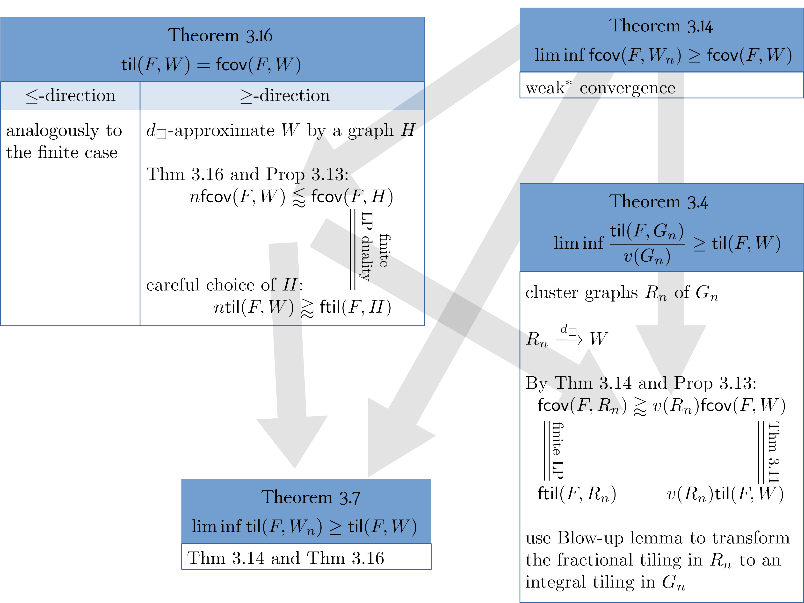
Figure 4.1 shows the dependencies and the key steps in the proofs of our main results.
Refer to caption
Figure 4.1. Main proof steps and dependencies of main results from Section 3.

4.1. Proof of Theorem 3.14

Without loss of generality let us assume that 𝔠n​⟶w∗​𝔠\mathfrak{c}_{n}\overset{\mathrm{w}^{*}}{\;\longrightarrow\;}\mathfrak{c}. In order to show that 𝔠\mathfrak{c} is a fractional FF-cover of WW, we need to show that for any measurable subsets A1,…,Ak⊂ΩA_{1},\ldots,A_{k}\subset\Omega for which there are numbers α1,…,αk\alpha_{1},\ldots,\alpha_{k}, ∑αi<1\sum\alpha_{i}<1 with 𝔠↾Ai<αi\mathfrak{c}_{\restriction A_{i}}<\alpha_{i}, we have ∫(x1,…,xk)∈∏AiW⊗F​(x1,…,xk)​𝖽​νk=0\int_{(x_{1},\ldots,x_{k})\in\prod A_{i}}W^{\otimes F}(x_{1},\ldots,x_{k})\>\mathsf{d}\nu^{k}=0. Let a=1−∑αia=1-\sum\alpha_{i}. Suppose for contradiction that ∫(x1,…,xk)∈∏AiW⊗F​(x1,…,xk)​𝖽​νk>0\int_{(x_{1},\ldots,x_{k})\in\prod A_{i}}W^{\otimes F}(x_{1},\ldots,x_{k})\>\mathsf{d}\nu^{k}>0. Let ξ>0\xi>0 be such that the set

𝐗={𝐱∈∏iAi:W⊗F​(𝐱)>ξ}\mathbf{X}=\left\{\mathbf{x}\in\prod_{i}A_{i}:W^{\otimes F}\left(\mathbf{x}\right)>\xi\right\}

has positive νk\nu^{k}-measure. Since kk-dimensional boxes generate the sigma-algebra on Ωk\Omega^{k}, for each d>0d>0 we can find sets B1⊂A1,…,Bk⊂AkB_{1}\subset A_{1},\ldots,B_{k}\subset A_{k} of positive measure such that

(4.1) νk​(𝐗∩∏iBi)≥(1−d)​∏iν⁡(Bi).\nu^{k}\left(\mathbf{X}\cap\prod_{i}B_{i}\right)\geq(1-d)\prod_{i}\nu(B_{i})\;.

Let us fix such sets for d:=(a/12​k)kd:=(\nicefrac{{a}}{{12k}})^{k}.

Let us take N1N_{1} such that for each n>N1n>N_{1} we have ‖W−Wn‖□<(a/13​k)k+2⋅∏iν⁡(Bi)⋅ξ\|W-W_{n}\|_{\square}<(\nicefrac{{a}}{{13k}})^{k+2}\cdot\prod_{i}\nu(B_{i})\cdot\xi. Lemma 2.2 tells us that for each collection D1,…,DkD_{1},\ldots,D_{k} of measurable subsets of Ω\Omega we have

(4.2) |∫(x1,…,xk)∈∏DiWn⊗F​(x1,…,xk)​𝖽​νk−∫(x1,…,xk)∈∏DiW⊗F​(x1,…,xk)​𝖽​νk|<(a/13​k)k⋅∏iν⁡(Bi)⋅ξ.\left|\int_{(x_{1},\ldots,x_{k})\in\prod D_{i}}W_{n}^{\otimes F}(x_{1},\ldots,x_{k})\>\mathsf{d}\nu^{k}-\int_{(x_{1},\ldots,x_{k})\in\prod D_{i}}W^{\otimes F}(x_{1},\ldots,x_{k})\>\mathsf{d}\nu^{k}\right|<(\nicefrac{{a}}{{13k}})^{k}\cdot\prod_{i}\nu(B_{i})\cdot\xi\;.

Since 𝔠n​⟶w∗​𝔠\mathfrak{c}_{n}\overset{\mathrm{w}^{*}}{\;\longrightarrow\;}\mathfrak{c}, there exists a number N2N_{2} such that for each n>N2n>N_{2} we have

(4.3) ∫x∈Bi𝔠n​(x)​𝑑ν≤∫x∈Bi𝔠⁡(x)+a3​k​𝑑ν≤ν⁡(Bi)​(αi+a3​k)for each i=1,…,k.\int_{x\in B_{i}}\mathfrak{c}_{n}(x)\>\mathsf{d}\nu\leq\int_{x\in B_{i}}\mathfrak{c}(x)+\frac{a}{3k}\>\mathsf{d}\nu\leq\nu(B_{i})\left(\alpha_{i}+\frac{a}{3k}\right)\quad\mbox{for each $i=1,\ldots,k$.}

Now, fix n>max⁡(N1,N2)n>\max(N_{1},N_{2}). For i=1,…,ki=1,\ldots,k, define Di=Bi∩𝔠n−1​([0,αi+2​a/3​k])D_{i}=B_{i}\cap\mathfrak{c}_{n}^{-1}\left([0,\alpha_{i}+\nicefrac{{2a}}{{3k}}]\right). Then we have

∫x∈Bi𝔠n​(x)​𝑑ν\displaystyle\int_{x\in B_{i}}\mathfrak{c}_{n}(x)\>\mathsf{d}\nu =\displaystyle= ∫x∈Di𝔠n​(x)​𝑑ν+∫x∈Bi∖Di𝔠n​(x)​𝑑ν\displaystyle\int_{x\in D_{i}}\mathfrak{c}_{n}(x)\>\mathsf{d}\nu+\int_{x\in B_{i}\setminus D_{i}}\mathfrak{c}_{n}(x)\>\mathsf{d}\nu
≥\displaystyle\geq ν⁡(Di)⋅0+ν⁡(Bi∖Di)⋅(αi+2​a/3​k)\displaystyle\nu(D_{i})\cdot 0+\nu(B_{i}\setminus D_{i})\cdot\left(\alpha_{i}+\nicefrac{{2a}}{{3k}}\right)
=\displaystyle= ν⁡(Bi)​(αi+2​a/3​k−ν⁡(Di)ν⁡(Bi)⋅(αi+2​a/3​k)).\displaystyle\nu(B_{i})\left(\alpha_{i}+\nicefrac{{2a}}{{3k}}-\frac{\nu(D_{i})}{\nu(B_{i})}\cdot\left(\alpha_{i}+\nicefrac{{2a}}{{3k}}\right)\right)\;.

Plugging this into (4.3) we get

ν⁡(Bi)​(αi+2​a/3​k−2​ν⁡(Di)ν⁡(Bi))≤ν⁡(Bi)​(αi+a/3​k),\nu(B_{i})\left(\alpha_{i}+\nicefrac{{2a}}{{3k}}-2\frac{\nu(D_{i})}{\nu(B_{i})}\right)\leq\nu(B_{i})\left(\alpha_{i}+\nicefrac{{a}}{{3k}}\right)\;,

and consequently,

(4.4) ν⁡(Di)≥a6​k⋅ν⁡(Bi).\nu(D_{i})\geq\frac{a}{6k}\cdot\nu(B_{i})\;.

Observe also that for each 𝐱∈∏Di\mathbf{x}\in\prod D_{i} we have ∑i𝔠n​(𝐱i)≤∑i(αi+2​a/3​k)=1−a/3<1\sum_{i}\mathfrak{c}_{n}(\mathbf{x}_{i})\leq\sum_{i}\left(\alpha_{i}+\nicefrac{{2a}}{{3k}}\right)=1-\nicefrac{{a}}{{3}}<1. Since 𝔠n\mathfrak{c}_{n} is a fractional FF-cover of WnW_{n}, we conclude that

(4.5) ∫(x1,⋯,xk)∈∏DiWn⊗F​(x1,…,xk)​𝖽​νk=0.\int_{(x_{1},\cdots,x_{k})\in\prod D_{i}}W_{n}^{\otimes F}(x_{1},\ldots,x_{k})\>\mathsf{d}\nu^{k}=0\;.

On the other hand,

∫(x1,⋯,xk)∈∏DiWn⊗F​(x1,…,xk)​𝖽​νk\displaystyle\int_{(x_{1},\cdots,x_{k})\in\prod D_{i}}W_{n}^{\otimes F}(x_{1},\ldots,x_{k})\>\mathsf{d}\nu^{k} ≥\displaystyle\geq ∫(x1,⋯,xk)∈𝐗∩∏Diξ​𝖽​νk\displaystyle\int_{(x_{1},\cdots,x_{k})\in\mathbf{X}\cap\prod D_{i}}\xi\>\mathsf{d}\nu^{k}
by (4.1) ≥\displaystyle\geq (∏iν⁡(Di)−d​∏iν⁡(Bi))​ξ\displaystyle\left(\prod_{i}\nu(D_{i})-d\prod_{i}\nu(B_{i})\right)\xi
by (4.4) ≥\displaystyle\geq (a/12​k)k​∏iν⁡(Bi)⋅ξ.\displaystyle(\nicefrac{{a}}{{12k}})^{k}\prod_{i}\nu(B_{i})\cdot\xi\;.

This, together with (4.5) contradicts (4.2).

4.2. Proof of Theorem 3.16

We split the proof into the easy “≤\leq”-part and the difficult “≥\geq”-part. The former is given in Proposition 4.1 and its proof is a straightforward modification of the finite version. The latter is given in Proposition 4.2. In the proof of Proposition 4.2 we first approximate a graphon by a finite graph on which we use finite LP-duality as a black-box.

We remark that this approach seems ad-hoc and it is reasonable to ask for a more conceptual proof. Indeed, as was pointed out to us by an anonymous referee, there is fairly rich literature on “algebraic infinite-dimensional duality” (see [2] for a survey). This theory would certainly not be able to give the results we need. The referee also pointed out to us “topological infinite-dimensional duality” developed in [7] which they suggested might provide a blackbox proof of Theorem 3.16. We were, however, unable to apply this theory in our setting.

Proposition 4.1.

Suppose that W:Ω2→[0,1]W:\Omega^{2}\rightarrow[0,1] is a graphon defined on Ω\Omega and FF is a graph on the vertex set [k][k]. Suppose that 𝔠:Ω→[0,1]\mathfrak{c}:\Omega\rightarrow[0,1] is a fractional FF-cover of WW and that 𝔱:Ωk→[0,1]\mathfrak{t}:\Omega^{k}\rightarrow[0,1] is an FF-tiling in WW. Then ‖𝔱‖≤‖𝔠‖\|\mathfrak{t}\|\leq\|\mathfrak{c}\|.

Proof.

We have

‖𝔱‖\displaystyle\|\mathfrak{t}\| =\displaystyle=
by (3.3) =\displaystyle= ∫(x1,…,xk)∈ℱF​(W)𝔱⁡(x1,…,xk)​𝖽​νk\displaystyle\int_{\left(x_{1},\ldots,x_{k}\right)\in\mathcal{F}_{F}(W)}\mathfrak{t}\left(x_{1},\ldots,x_{k}\right)\>\mathsf{d}\nu^{k}
Definition 3.12 ≤\displaystyle\leq ∫(x1,…,xk)∈ℱF​(W)𝔱⁡(x1,…,xk)​(∑i=1k𝔠⁡(xi))​𝖽​νk\displaystyle\int_{\left(x_{1},\ldots,x_{k}\right)\in\mathcal{F}_{F}(W)}\mathfrak{t}\left(x_{1},\ldots,x_{k}\right)\left(\sum_{i=1}^{k}\mathfrak{c}\left(x_{i}\right)\right)\>\mathsf{d}\nu^{k}
=\displaystyle= ∫x∈Ω(𝔠⁡(x)​∑i=1k∫(x1,…,,xi−1,xi+1,…,xk)∈Ωk−1(x1,…,xi−1,x,xi+1,…,xk)∈ℱF​(W)𝔱⁡(x1,…,xi−1,x,xi+1,…,xk))​𝑑ν\displaystyle\int_{x\in\Omega}\left(\mathfrak{c}(x)\sum_{i=1}^{k}\int_{\begin{subarray}{c}\left(x_{1},\ldots,,x_{i-1},x_{i+1},\ldots,x_{k}\right)\in\Omega^{k-1}\\ \left(x_{1},\ldots,x_{i-1},x,x_{i+1},\ldots,x_{k}\right)\in\mathcal{F}_{F}(W)\end{subarray}}\mathfrak{t}\left(x_{1},\ldots,x_{i-1},x,x_{i+1},\ldots,x_{k}\right)\right)\>\mathsf{d}\nu
by (3.4) ≤\displaystyle\leq ∫x∈Ω𝔠⁡(x)​𝑑ν,\displaystyle\int_{x\in\Omega}\mathfrak{c}(x)\>\mathsf{d}\nu\;,

as was needed. ∎

Proposition 4.2.

Suppose that W:Ω2→[0,1]W:\Omega^{2}\rightarrow[0,1] is a graphon defined on Ω\Omega and FF is a graph on the vertex set [k][k]. Then for an arbitrary ϵ>0\epsilon>0 there exists an FF-tiling 𝔱:Ωk→[0,1]\mathfrak{t}:\Omega^{k}\rightarrow[0,1] in WW with ‖𝔱‖≥𝖿𝖼𝗈𝗏⁡(F,W)−ϵ\|\mathfrak{t}\|\geq\mathsf{fcov}(F,W)-\epsilon.

Proof.

For each n=1,2,…n=1,2,\ldots, we find a suitable kn∈ℕk_{n}\in\mathbb{N}, a partition Ω=Ω1(n)⊔Ω2(n)⊔…⊔Ωkn(n)\Omega=\Omega_{1}^{(n)}\sqcup\Omega_{2}^{(n)}\sqcup\ldots\sqcup\Omega_{k_{n}}^{(n)} into knk_{n} sets of measure 1kn\frac{1}{k_{n}} each, and a graphon Wn:Ω2→[0,1]W_{n}:\Omega^{2}\rightarrow[0,1] such that WnW_{n} is constant on each rectangle Ωi(n)×Ωj(n)\Omega_{i}^{(n)}\times\Omega_{j}^{(n)} (i,j∈[kn]i,j\in[k_{n}]), and ‖W−Wn‖1<1/n\|W-W_{n}\|_{1}<\nicefrac{{1}}{{n}}. This is possible as step functions with square steps are dense in ℒ1​(Ω2)\mathcal{L}^{1}(\Omega^{2}). We shall now modify the graphons WnW_{n} in two steps.

First, let Wn′:Ω2→[0,1]W_{n}^{\prime}:\Omega^{2}\rightarrow[0,1] be defined as

Wn′​(x,y)={Wn​(x,y)if Wn​(x,y)≥1/n0otherwise.W_{n}^{\prime}(x,y)=\begin{cases}W_{n}(x,y)&\mbox{if $W_{n}(x,y)\geq\sqrt{\nicefrac{{1}}{{n}}}$}\\ 0&\mbox{otherwise}\end{cases}\;.

This way, we have that

(4.6) ‖Wn−Wn′‖1<1/n.\|W_{n}-W_{n}^{\prime}\|_{1}<\sqrt{\nicefrac{{1}}{{n}}}\;.

For a fixed nn, we say that a rectangle Ωi(n)×Ωj(n)\Omega_{i}^{(n)}\times\Omega_{j}^{(n)} is shoddy if the measure of the set

(supp​Wn′∖supp​W)∩(Ωi(n)×Ωj(n))\left(\mathrm{supp\>}W_{n}^{\prime}\setminus\mathrm{supp\>}W\right)\cap\left(\Omega_{i}^{(n)}\times\Omega_{j}^{(n)}\right)

is at least 1/n4⋅1kn2\sqrt[4]{\nicefrac{{1}}{{n}}}\cdot\frac{1}{k_{n}^{2}}. Note that at each point of supp​Wn′∖supp​W\mathrm{supp\>}W_{n}^{\prime}\setminus\mathrm{supp\>}W the difference between WnW_{n} and WW is at least 1/n\sqrt{\nicefrac{{1}}{{n}}}. This gives that ν2​(supp​Wn′∖supp​W)≤‖Wn−W‖11/n≤1/n\nu^{2}\left(\mathrm{supp\>}W_{n}^{\prime}\setminus\mathrm{supp\>}W\right)\leq\frac{\|W_{n}-W\|_{1}}{\sqrt{\nicefrac{{1}}{{n}}}}\leq\sqrt{\nicefrac{{1}}{{n}}}, which in turn implies that at most 1/n4⋅kn2\sqrt[4]{\nicefrac{{1}}{{n}}}\cdot k_{n}^{2} rectangles Ωi(n)×Ωj(n)\Omega_{i}^{(n)}\times\Omega_{j}^{(n)} are shoddy. Let us define

Wn′′​(x,y)={0(x,y) lies in a shoddy rectangleWn′​(x,y)otherwise.W_{n}^{\prime\prime}(x,y)=\begin{cases}0&\mbox{$(x,y)$ lies in a shoddy rectangle}\\ W^{\prime}_{n}(x,y)&\mbox{otherwise}\end{cases}\;.

Observe that shoddy rectangles are symmetric, so Wn′′W_{n}^{\prime\prime} is indeed a graphon. We changed Wn′′W^{\prime\prime}_{n} on a set of measure at most 1/n4\sqrt[4]{\nicefrac{{1}}{{n}}} which gives that

(4.7) ‖Wn′−Wn′′‖1≤1/n4.\|W_{n}^{\prime}-W_{n}^{\prime\prime}\|_{1}\leq\sqrt[4]{\nicefrac{{1}}{{n}}}\;.

To summarize, we ended up with a graphon Wn′′W^{\prime\prime}_{n} which is a step-function on the rectangles Ωi(n)×Ωj(n)\Omega_{i}^{(n)}\times\Omega_{j}^{(n)} and for which we have

‖Wn′′−W‖1≤‖Wn−W‖1+‖Wn′−Wn‖1+‖Wn′′−Wn′‖1​<(4.6),(4.7)​1n+1/n+1/n4⟶n→∞0.\|W_{n}^{\prime\prime}-W\|_{1}\leq\|W_{n}-W\|_{1}+\|W_{n}^{\prime}-W_{n}\|_{1}+\|W^{\prime\prime}_{n}-W_{n}^{\prime}\|_{1}\overset{\eqref{eq:WWone},\eqref{eq:WoneWtwo}}{<}\frac{1}{n}+\sqrt{\nicefrac{{1}}{{n}}}+\sqrt[4]{\nicefrac{{1}}{{n}}}\quad\overset{n\rightarrow\infty}{\;\longrightarrow\;}\quad 0\;.

Since the ℒ1​(Ω2)\mathcal{L}^{1}(\Omega^{2})-norm is stronger than the cut-norm, we have that the graphons (Wn′′)(W_{n}^{\prime\prime}) converge to WW. In particular, Theorem 3.14 tells us that lim infn𝖿𝖼𝗈𝗏⁡(F,Wn′′)≥𝖿𝖼𝗈𝗏⁡(F,W)\liminf_{n}\mathsf{fcov}(F,W_{n}^{\prime\prime})\geq\mathsf{fcov}(F,W). Let N1N_{1} be such that for each n≥N1n\geq N_{1} we have 𝖿𝖼𝗈𝗏⁡(F,Wn′′)≥𝖿𝖼𝗈𝗏⁡(F,W)−ϵ/2\mathsf{fcov}(F,W_{n}^{\prime\prime})\geq\mathsf{fcov}(F,W)-\nicefrac{{\epsilon}}{{2}}. Let N2=⌈k/ϵ⌉8N_{2}=\lceil\nicefrac{{k}}{{\epsilon}}\rceil^{8}. Now, fix an arbitrary number N≥max⁡(N1,N2)N\geq\max(N_{1},N_{2}), and consider the graphon WN′′W_{N}^{\prime\prime}. This graphon represents a finite graph on the vertex set V={1,…,kN}V=\{1,\ldots,k_{N}\}. We call this graph HH. We forget the edge-weights, that is we put an edge i​jij in HH whenever WN′′W_{N}^{\prime\prime} is positive on Ωi(N)×Ωj(N)\Omega_{i}^{(N)}\times\Omega_{j}^{(N)}. By Proposition 3.13, 𝖿𝖼𝗈𝗏⁡(F,H)=kN⋅𝖿𝖼𝗈𝗏⁡(F,WN′′)\mathsf{fcov}(F,H)=k_{N}\cdot\mathsf{fcov}(F,W_{N}^{\prime\prime}).

The LP-duality of finite graphs tells us that we can find a fractional FF-tiling 𝔱H:Vk→[0,1]\mathfrak{t}_{H}:V^{k}\rightarrow[0,1] on HH with ∑𝔱H​(v1,…,vk)=𝖿𝖼𝗈𝗏⁡(F,H)\sum\mathfrak{t}_{H}(v_{1},\ldots,v_{k})=\mathsf{fcov}(F,H). It is easy to transform 𝔱H\mathfrak{t}_{H} to a fractional FF-tiling 𝔱:Ωk→[0,∞)\mathfrak{t}:\Omega^{k}\rightarrow[0,\infty) on WN′′W_{N}^{\prime\prime} by defining 𝔱\mathfrak{t} to be the constant kN⋅𝔱H​(v1,…,vk)k_{N}\cdot\mathfrak{t}_{H}(v_{1},\ldots,v_{k}) on the entire rectangle ∏iΩvi(N)\prod_{i}\Omega_{v_{i}}^{(N)} (for each OPENv1,v2,…,vk∈[kN])v_{1},v_{2},\ldots,v_{k}\in[k_{N}]). Then 𝔱\mathfrak{t} has weight 1kN​∑𝔱H​(v1,…,vk)=𝖿𝖼𝗈𝗏⁡(F,WN′′)\frac{1}{k_{N}}\sum\mathfrak{t}_{H}(v_{1},\ldots,v_{k})=\mathsf{fcov}(F,W_{N}^{\prime\prime}). The function 𝔱\mathfrak{t} is not necessarily a fractional FF-tiling on WW, as condition (3.3) may be violated due to values at points P=supp⁡((WN′′)⊗F)∖supp⁡(W⊗F)P=\mathrm{supp\>}\left(\left(W_{N}^{\prime\prime}\right)^{\otimes F}\right)\setminus\mathrm{supp\>}\left(W^{\otimes F}\right). We have

(4.8) P⊂⋃i<j,i​j∈E⁡(F)πi​j−1​(supp​Wn′′∖supp​W).P\subset\bigcup_{i<j,ij\in E(F)}\pi_{ij}^{-1}\left(\mathrm{supp\>}W_{n}^{\prime\prime}\setminus\mathrm{supp\>}W\right)\;.

Let 𝔱′\mathfrak{t}^{\prime} be zero on PP, and equal to 𝔱\mathfrak{t} elsewhere. Then 𝔱′\mathfrak{t}^{\prime} is a fractional FF-tiling on WW.

Since supp​Wn′′∖supp​W\mathrm{supp\>}W_{n}^{\prime\prime}\setminus\mathrm{supp\>}W is disjoint from points of shoddy rectangles, we have that for each choice of v1,…,vkv_{1},\ldots,v_{k}, the product set ∏i=1kΩvi(N)\prod_{i=1}^{k}\Omega_{v_{i}}^{(N)} satisfies

νk​(∏i=1kΩvi(N)∩P)\displaystyle\nu^{k}\left(\prod_{i=1}^{k}\Omega_{v_{i}}^{(N)}\cap P\right) ≤(4.8)\displaystyle\overset{\eqref{eq:Pij}}{\leq} ∑ℓ<j,i​j∈E⁡(F)νk​(∏i=1kΩvi(N)∩πℓ​j−1​(supp​WN′′∖supp​W))\displaystyle\sum_{\ell<j,ij\in E(F)}\nu^{k}\left(\prod_{i=1}^{k}\Omega_{v_{i}}^{(N)}\cap\pi_{\ell j}^{-1}\left(\mathrm{supp\>}W_{N}^{\prime\prime}\setminus\mathrm{supp\>}W\right)\right)
≤\displaystyle\leq νk​(∏i=1kΩvi(N))​(k2)​1/N4.\displaystyle\nu^{k}\left(\prod_{i=1}^{k}\Omega_{v_{i}}^{(N)}\right)\binom{k}{2}\sqrt[4]{\nicefrac{{1}}{{N}}}\;.

Using that 𝔱\mathfrak{t} is constant on ∏i=1kΩvi(N)\prod_{i=1}^{k}\Omega_{v_{i}}^{(N)}, we get that

∫(x1,…,xk)∈∏i=1kΩvi(N)𝔱′​(x1,…,xk)​𝖽​νk≥(1−(k2)​1/N4)​∫(x1,…,xk)∈∏i=1kΩvi𝔱⁡(x1,…,xk)​𝖽​νk.\int_{(x_{1},\ldots,x_{k})\in\prod_{i=1}^{k}\Omega_{v_{i}}^{(N)}}\mathfrak{t}^{\prime}(x_{1},\ldots,x_{k})\>\mathsf{d}\nu^{k}\geq\left(1-\tbinom{k}{2}\sqrt[4]{\nicefrac{{1}}{{N}}}\right)\int_{(x_{1},\ldots,x_{k})\in\prod_{i=1}^{k}\Omega_{v_{i}}}\mathfrak{t}(x_{1},\ldots,x_{k})\>\mathsf{d}\nu^{k}\;.

Summing over all product sets ∏i=1kΩvi(N)\prod_{i=1}^{k}\Omega_{v_{i}}^{(N)} we get that 𝔱′\mathfrak{t}^{\prime} is a fractional FF-tiling on WW with

∫(x1,…,xk)∈Ωk𝔱′​(x1,…,xk)​𝖽​νk\displaystyle\int_{(x_{1},\ldots,x_{k})\in\Omega^{k}}\mathfrak{t}^{\prime}(x_{1},\ldots,x_{k})\>\mathsf{d}\nu^{k} ≥(1−(k2)​1/N4)​∫(x1,…,xk)∈Ωk𝔱⁡(x1,…,xk)​𝖽​νk\displaystyle\geq\left(1-\tbinom{k}{2}\sqrt[4]{\nicefrac{{1}}{{N}}}\right)\int_{(x_{1},\ldots,x_{k})\in\Omega^{k}}\mathfrak{t}(x_{1},\ldots,x_{k})\>\mathsf{d}\nu^{k}
≥∫(x1,…,xk)∈Ωk𝔱⁡(x1,…,xk)​𝖽​νk−ϵ2\displaystyle\geq\int_{(x_{1},\ldots,x_{k})\in\Omega^{k}}\mathfrak{t}(x_{1},\ldots,x_{k})\>\mathsf{d}\nu^{k}-\frac{\epsilon}{2}
=𝖿𝖼𝗈𝗏⁡(F,WN′′)−ϵ2≥𝖿𝖼𝗈𝗏⁡(F,W)−ϵ,\displaystyle=\mathsf{fcov}(F,W_{N}^{\prime\prime})-\frac{\epsilon}{2}\geq\mathsf{fcov}(F,W)-\epsilon\;,

as was needed. ∎

4.3. Proof of Theorem 3.7

By Theorem 3.16 it suffices to prove that lim infn𝖿𝖼𝗈𝗏⁡(F,Wn)≥𝖿𝖼𝗈𝗏⁡(F,W)\liminf_{n}\mathsf{fcov}(F,W_{n})\geq\mathsf{fcov}(F,W). This, however, is the subject of Corollary 3.15.

4.4. Proof of Theorem 3.4

For simplicity, let us assume that v⁡(Gn)=nv(G_{n})=n. Suppose that ϵ>0\epsilon>0 is arbitrary. We want to show that for nn sufficiently large, 𝗍𝗂𝗅⁡(F,Gn)≥(𝗍𝗂𝗅⁡(F,W)−ϵ)​n=(𝖿𝖼𝗈𝗏⁡(F,W)−ϵ)​n\mathsf{til}(F,G_{n})\geq(\mathsf{til}(F,W)-\epsilon)n=(\mathsf{fcov}(F,W)-\epsilon)n (where the last equality uses Theorem 3.16). Let δ>0\delta>0 be such that whenever UU is a graphon of cut-distance at most δ\delta from WW we have that

(4.9) 𝖿𝖼𝗈𝗏⁡(F,U)≥𝖿𝖼𝗈𝗏⁡(F,W)−ϵ/3.\mathsf{fcov}(F,U)\geq\mathsf{fcov}(F,W)-\nicefrac{{\epsilon}}{{3}}\;.

Such a number δ\delta exists by Corollary 3.15. Let d=δ/10d=\nicefrac{{\delta}}{{10}}. Let ϵ1\epsilon_{1} be given by Lemma 2.8 for the error parameter γ=ϵ/10\gamma=\nicefrac{{\epsilon}}{{10}} and density d/2\nicefrac{{d}}{{2}}. Let ϵ0\epsilon_{0} be given by Lemma 2.7 for the input parameter β=0.1\beta=0.1 and error parameter ϵ1\epsilon_{1}. Set ϵ2=min⁡(ϵ0,δ/10)\epsilon_{2}=\min(\epsilon_{0},\nicefrac{{\delta}}{{10}}). Lemma 2.6 with error parameter ϵ2\epsilon_{2} gives us a bound LL on the complexity of partitions.

Suppose nn is large enough, so that we have

(4.10) dist□​(WGn,W)<δ/2.\mathrm{dist}_{\square}(W_{G_{n}},W)<\nicefrac{{\delta}}{{2}}\;.

Consider a cluster graph RnR_{n} corresponding to a (ϵ2,d)(\epsilon_{2},d)-regularization of the graph GnG_{n}. Let 𝒱=(V1,…,Vℓ)\mathcal{V}=(V_{1},\ldots,V_{\ell}) be the corresponding partition of V⁡(Gn)V(G_{n}) into clusters, with ℓ≤L\ell\leq L. Let m=|V1|m=|V_{1}|. By (2.2) we have dist□​(WGn,WRn)<δ/2\mathrm{dist}_{\square}(W_{G_{n}},W_{R_{n}})<\nicefrac{{\delta}}{{2}}. Combining with (4.10), triangle inequality gives dist□​(W,WRn)<δ\mathrm{dist}_{\square}(W,W_{R_{n}})<\delta. In particular, (4.9) can be applied to WRnW_{R_{n}}. Proposition 3.13 then gives that 𝖿𝖼𝗈𝗏⁡(F,Rn)=ℓ⋅𝖿𝖼𝗈𝗏⁡(F,WRn)≥ℓ⁡(𝖿𝖼𝗈𝗏⁡(F,W)−ϵ/3)\mathsf{fcov}(F,R_{n})=\ell\cdot\mathsf{fcov}(F,W_{R_{n}})\geq\ell\left(\mathsf{fcov}(F,W)-\nicefrac{{\epsilon}}{{3}}\right). We ignore the edge weights in RnR_{n}. We apply the (standard) LP duality on RnR_{n}. We get a fractional FF-tiling 𝔱Rn:[ℓ]k→[0,1]\mathfrak{t}_{R_{n}}:[\ell]^{k}\rightarrow[0,1]. We now delete from 𝔱Rn\mathfrak{t}_{R_{n}} very small weights. Formally, for a kk-tuple 𝐯∈[ℓ]k\mathbf{v}\in[\ell]^{k} we define 𝔱Rn′​(𝐯)\mathfrak{t}^{\prime}_{R_{n}}(\mathbf{v}) to be 0 if 𝔱(𝐯)Rn<ϵ/(10​ℓk−1)\mathfrak{t}{}_{R_{n}}(\mathbf{v})<\nicefrac{{\epsilon}}{{\left(10\ell^{k-1}\right)}} and to be 𝔱Rn​(𝐯)\mathfrak{t}_{R_{n}}(\mathbf{v}) otherwise. Observe that ∥𝔱′Rn∥≥∥𝔱Rn∥−ϵ​ℓ/10\|\mathfrak{t}^{\prime}{}_{R_{n}}\|\geq\|\mathfrak{t}{}_{R_{n}}\|-\nicefrac{{\epsilon\ell}}{{10}}. For each copy F~\tilde{F} of the graph FF inside RnR_{n} which is in the support of 𝔱′Rn\mathfrak{t}^{\prime}{}_{R_{n}}, consider an arbitrary integer mF~m_{\tilde{F}} in the range between [(1−ϵ/10)⋅𝔱′(F~)Rn⋅m,𝔱′(F~)Rn⋅m]\left[\left(1-\nicefrac{{\epsilon}}{{10}}\right)\cdot\mathfrak{t}^{\prime}{}_{R_{n}}(\tilde{F})\cdot m,\mathfrak{t}^{\prime}{}_{R_{n}}(\tilde{F})\cdot m\right]. Since we can assume that nn is sufficiently large, for the gap between the endpoints of this range we have

ϵ10⋅𝔱′(F~)Rn⋅m≥ϵ10⋅ϵ10​ℓk−1⋅(1−ϵ2)​nℓ≥1.\frac{\epsilon}{10}\cdot\mathfrak{t}^{\prime}{}_{R_{n}}(\tilde{F})\cdot m\geq\frac{\epsilon}{10}\cdot\frac{\epsilon}{10\ell^{k-1}}\cdot\frac{(1-\epsilon_{2})n}{\ell}\geq 1\;.

In particular, we can indeed find an integer mF~m_{\tilde{F}} in the specified range.

Now, for each cluster ViV_{i}, we construct a partition of ViV_{i} into sets Vi,0⊔⨆Vi,F~V_{i,0}\sqcup\bigsqcup V_{i,\tilde{F}} where F~\tilde{F} runs over all copies of FF in RnR_{n} that touch the vertex ii. In this partition, the size of each set Vi,F~V_{i,\tilde{F}} is mF~m_{\tilde{F}}, and Vi,0V_{i,0} is the remainder. Since 𝔱Rn′\mathfrak{t}^{\prime}_{R_{n}} is an FF-tiling mF~F~:F~∋i≤∑F~:F~∋i𝔱′(F~)Rn⋅m≤m{}_{\tilde{F}:\tilde{F}\ni i}m_{\tilde{F}}\leq\sum_{\tilde{F}:\tilde{F}\ni i}\mathfrak{t}^{\prime}{}_{R_{n}}(\tilde{F})\cdot m\leq m. That means that at least one such partition exists. Among all such partitions Vi,0⊔⨆Vi,F~V_{i,0}\sqcup\bigsqcup V_{i,\tilde{F}}, consider a random one.

Suppose that this way we randomly partitioned all the clusters V1,…,VℓV_{1},\ldots,V_{\ell}. For a given copy F~\tilde{F} of FF in RnR_{n} in the support of 𝔱Rn′\mathfrak{t}^{\prime}_{R_{n}}, we set up a random variable XF~X_{\tilde{F}} as follows. If for each edge i​j∈F~ij\in\tilde{F} the pair (Vi,F~,Vj,F~)(V_{i,\tilde{F}},V_{j,\tilde{F}}) is ϵ1\epsilon_{1}-regular, we set XF~=(1−ϵ/10)​mF~X_{\tilde{F}}=(1-\nicefrac{{\epsilon}}{{10}})m_{\tilde{F}}. If there exists an edge i​j∈F~ij\in\tilde{F} for which the pair (Vi,F~,Vj,F~)(V_{i,\tilde{F}},V_{j,\tilde{F}}) fails to be ϵ1\epsilon_{1}-regular, we set XF~=0X_{\tilde{F}}=0. Lemma 2.8 gives that one can always find an FF-tiling of size XF~X_{\tilde{F}} in Gn​[⋃i∈V⁡(F~)Vi,F~]G_{n}\left[\bigcup_{i\in V(\tilde{F})}V_{i,\tilde{F}}\right].

Lemma 2.7 implies that 𝐄⁡[XF~]≥exp⁡(−2​e​(F)​0.1mF~)​(1−ϵ/10)​mF~≥(1−ϵ/5)​mF~\mathbf{E}\left[X_{\tilde{F}}\right]\geq\exp\left(-2e(F)0.1^{m_{\tilde{F}}}\right)(1-\nicefrac{{\epsilon}}{{10}})m_{\tilde{F}}\geq(1-\nicefrac{{\epsilon}}{{5}})m_{\tilde{F}}. By linearity of expectation,

𝐄⁡[∑F~XF~]\displaystyle\mathbf{E}\left[\sum_{\tilde{F}}X_{\tilde{F}}\right] ≥\displaystyle\geq (1−ϵ/5)∑F~(1−ϵ/10)⋅𝔱′(F~)Rn⋅m≥(1−ϵ/3)∥𝔱Rn′∥m\displaystyle(1-\nicefrac{{\epsilon}}{{5}})\sum_{\tilde{F}}\left(1-\nicefrac{{\epsilon}}{{10}}\right)\cdot\mathfrak{t}^{\prime}{}_{R_{n}}(\tilde{F})\cdot m\geq(1-\nicefrac{{\epsilon}}{{3}})\|\mathfrak{t}^{\prime}_{R_{n}}\|m
≥\displaystyle\geq (1−ϵ/3)∥𝔱∥Rnm−ϵ​n/10.\displaystyle(1-\nicefrac{{\epsilon}}{{3}})\|\mathfrak{t}{}_{R_{n}}\|m-\nicefrac{{\epsilon n}}{{10}}\;.

So, let us fix one collection of partitions such that ∑F~XF~≥(1−ϵ/3)∥𝔱∥Rnm−ϵ​n/10\sum_{\tilde{F}}X_{\tilde{F}}\geq(1-\nicefrac{{\epsilon}}{{3}})\|\mathfrak{t}{}_{R_{n}}\|m-\nicefrac{{\epsilon n}}{{10}}. Then by the above there is an FF-tiling in GnG_{n} of size ∑F~XF~\sum_{\tilde{F}}X_{\tilde{F}}. Using the fact that 𝖿𝖼𝗈𝗏⁡(F,Rn)≥ℓ⁡(𝖿𝖼𝗈𝗏⁡(F,W)−ϵ/3)\mathsf{fcov}(F,R_{n})\geq\ell\left(\mathsf{fcov}(F,W)-\nicefrac{{\epsilon}}{{3}}\right), we obtain that 𝗍𝗂𝗅⁡(F,Gn)≥(𝖿𝖼𝗈𝗏⁡(F,W)−ϵ)​n\mathsf{til}(F,G_{n})\geq(\mathsf{fcov}(F,W)-\epsilon)n, as needed.

4.5. Proof of Proposition 3.8

Write k=v⁡(F)k=v(F). Given η>0\eta>0, let the number β\beta be given by the Removal lemma 2.5 for the graph FF and the parameters α=(η/2)k+2\alpha=\left(\nicefrac{{\eta}}{{2}}\right)^{k+2} and d=η/2d=\eta/2. Set δ=β​(η/2)4​k2/k2\delta=\beta(\eta/2)^{4k^{2}}/k^{2}.

Suppose now that UU is δ\delta-close to WW in the cut-norm. Let us fix an optimal fractional FF-cover 𝔠\mathfrak{c} of WW (recall Theorem 3.16 and (3.7)). Let U^\widehat{U} and 𝔠′\mathfrak{c}^{{}^{\prime}} be defined by

U^​(x,y)\displaystyle\widehat{U}(x,y) =\displaystyle= {U⁡(x,y)if U⁡(x,y)>η/20if U⁡(x,y)≤η/2,\displaystyle\begin{cases}U(x,y)&\mbox{if $U(x,y)>\eta/2$}\\ 0&\mbox{if $U(x,y)\leq\eta$}/2\end{cases}\;,
𝔠′​(x)\displaystyle\mathfrak{c}^{\prime}(x) =\displaystyle= max⁡(𝔠⁡(x)+η,1).\displaystyle\max\left(\mathfrak{c}(x)+\eta,1\right)\;.

Obviously, ‖U−U^‖1≤η/2\|U-\widehat{U}\|_{1}\leq\eta/2 and ‖𝔠′‖≤‖𝔠‖+η\|\mathfrak{c}^{\prime}\|\leq\|\mathfrak{c}\|+\eta. Let ℓ=⌈η−1⌉\ell=\lceil\eta^{-1}\rceil. Let us consider the sets AiA_{i}, i=1,…,ℓi=1,\ldots,\ell defined by Ai=𝔠−1[0,i/ℓ)A_{i}=\mathfrak{c}^{-1}[0,\nicefrac{{i}}{{\ell}}). Let X⊂ΩkX\subset\Omega^{k} be the set of points (x1,…,xk)(x_{1},\ldots,x_{k}) where U^(x1,…,xk)⊗F>0\widehat{U}{}^{\otimes F}(x_{1},\ldots,x_{k})>0 but ∑i𝔠′​(xi)<1\sum_{i}\mathfrak{c}^{\prime}(x_{i})<1. Let ℐ⊂ℕk\mathcal{I}\subset\mathbb{N}^{k} be the set of all kk-tuples of integers whose sum is ℓ\ell. We have |ℐ|≤(2η)k|\mathcal{I}|\leq\left(\frac{2}{\eta}\right)^{k}. Observe that

(4.11) X⊂⋃𝐢∈ℐA𝐢1×A𝐢2×⋯×A𝐢k.X\subset\bigcup_{\mathbf{i}\in\mathcal{I}}A_{\mathbf{i}_{1}}\times A_{\mathbf{i}_{2}}\times\cdots\times A_{\mathbf{i}_{k}}\;.

The next claim is crucial.

Claim.

For each kk-tuple 𝐢∈ℐ\mathbf{i}\in\mathcal{I}, we have for 𝐀=A𝐢1×A𝐢2×⋯×A𝐢k\mathbf{A}=A_{\mathbf{i}_{1}}\times A_{\mathbf{i}_{2}}\times\cdots\times A_{\mathbf{i}_{k}} that νk​(𝐀∩X)≤β\nu^{k}(\mathbf{A}\cap X)\leq\beta.

Proof.

Suppose for a contradiction that νk​(𝐀∩X)>β\nu^{k}(\mathbf{A}\cap X)>\beta. Therefore, we have

(4.12) ∫(x1,…,xk)∈𝐀U(x1,…,xk)⊗F𝖽νk≥∫(x1,…,xk)∈𝐀U^(x1,…,xk)⊗F𝖽νk≥(η/2)e⁡(F)⋅β>k2δ.\int_{(x_{1},\ldots,x_{k})\in\mathbf{A}}U{}^{\otimes F}(x_{1},\ldots,x_{k})\>\mathsf{d}\nu^{k}\geq\int_{(x_{1},\ldots,x_{k})\in\mathbf{A}}\widehat{U}{}^{\otimes F}(x_{1},\ldots,x_{k})\>\mathsf{d}\nu^{k}\geq\left(\nicefrac{{\eta}}{{2}}\right)^{e(F)}\cdot\beta>k^{2}\delta\;.

On the other hand, for each kk-tuple 𝐱∈𝐀\mathbf{x}\in\mathbf{A} we have ∑j𝔠⁡(𝐱j)<1\sum_{j}\mathfrak{c}(\mathbf{x}_{j})<1. Since 𝔠\mathfrak{c} is a fractional FF-cover of WW, we conclude that WF​(𝐱)=0W^{F}(\mathbf{x})=0. Therefore,

(4.13) ∫(x1,…,xk)∈𝐀W(x1,…,xk)⊗F𝖽νk=0.\int_{(x_{1},\ldots,x_{k})\in\mathbf{A}}W{}^{\otimes F}(x_{1},\ldots,x_{k})\>\mathsf{d}\nu^{k}=0\;.

Combining 4.12 and 4.13 with Lemma 2.2 we get that ‖U−W‖□>δ\|U-W\|_{\square}>\delta, which is a contradiction. ∎

We shall use tools introduced in Section 2.4. For each 𝐢∈ℐ\mathbf{i}\in\mathcal{I}, let U𝐢U_{\mathbf{i}} be the (A𝐢1,…,Ak)\left(A_{\mathbf{i}_{1}},\ldots,A_{k}\right)-partite version of U^\widehat{U} defined on an auxiliary measure space Ω𝐢=A𝐢1∐…∐A𝐢k\Omega_{\mathbf{i}}=A_{\mathbf{i}_{1}}\amalg\ldots\amalg A_{\mathbf{i}_{k}} with a measure νΩ𝐢\nu_{\Omega_{\mathbf{i}}}. The above Claim tells us that ∫(x1,…,xk)∈(Ω𝐢)kU𝐢^⊗F​𝖽​(νΩ𝐢)≤β\int_{(x_{1},\ldots,x_{k})\in\left(\Omega_{\mathbf{i}}\right)^{k}}\widehat{U_{\mathbf{i}}}^{\otimes F}\>\mathsf{d}\left(\nu_{\Omega_{\mathbf{i}}}\right)\leq\beta. The Removal Lemma (Lemma 2.5) tells us that there exists a set S𝐢⊂Ω𝐢2S_{\mathbf{i}}\subset\Omega_{\mathbf{i}}^{2} of Ω𝐢2\Omega_{\mathbf{i}}^{2}-measure at most α\alpha such that nullifying U𝐢^\widehat{U_{\mathbf{i}}} on S𝐢S_{\mathbf{i}} yields an FF-free graphon. Let B𝐢⊂Ω2B_{\mathbf{i}}\subset\Omega^{2} be the folded version of S𝐢S_{\mathbf{i}}. We have that ν2​(B𝐢)≤α\nu^{2}(B_{\mathbf{i}})\leq\alpha by (2.1). Let us now nullify U^\widehat{U} on B=⋃𝐢∈ℐB𝐢B=\bigcup_{\mathbf{i}\in\mathcal{I}}B_{\mathbf{i}}. The set BB has ν2\nu^{2}-measure at most |ℐ|⋅α≤2ηk⋅α≤η/2|\mathcal{I}|\cdot\alpha\leq\frac{2}{\eta^{k}}\cdot\alpha\leq\nicefrac{{\eta}}{{2}}, and thus the resulting graphon U∗U^{*} satisfies ‖U−U∗‖1≤η\|U-U^{*}\|_{1}\leq\eta. The nullification together with (4.11) tells us that 𝔠′\mathfrak{c}^{\prime} is a fractional FF-cover of U∗U^{*}. This finishes the proof.

4.6. Proof of Theorem 3.10

Suppose that a sequence of graphons (Wn)n\left(W_{n}\right)_{n} converges to a graphon WW in the cut-norm. We shall prove the statement in two steps:

(4.14) lim supn𝗍𝗂𝗅ϵ​(F,Wn)\displaystyle\limsup_{n}\mathsf{til}_{\epsilon}(F,W_{n}) ≥\displaystyle\geq 𝗍𝗂𝗅ϵ​(F,W),and\displaystyle\mathsf{til}_{\epsilon}(F,W)\;,\mbox{and}
(4.15) lim supn𝗍𝗂𝗅ϵ​(F,Wn)\displaystyle\limsup_{n}\mathsf{til}_{\epsilon}(F,W_{n}) ≤\displaystyle\leq 𝗍𝗂𝗅ϵ​(F,W).\displaystyle\mathsf{til}_{\epsilon}(F,W)\;.

(Note that by passing to a subsequence, we could turn the limit superior into a limit.)

First, let us prove (4.14). For each nn, suppose that Un≤WnU_{n}\leq W_{n} is an arbitrary graphon of ℒ1​(Ω2)\mathcal{L}^{1}(\Omega^{2})-norm at most ϵ\epsilon. Since the space of graphons is sequentially compact, let us consider the limit UU of a suitable subsequence (Uni)i\left(U_{n_{i}}\right)_{i}. Since Uni≤WniU_{n_{i}}\leq W_{n_{i}} for each ii, we also have U≤WU\leq W. Furthermore, since the ℒ1​(Ω2)\mathcal{L}^{1}(\Omega^{2})-norm is continuous with respect to the cut-distance, we have that the ℒ1​(Ω2)\mathcal{L}^{1}(\Omega^{2})-norm of UU is at most ϵ\epsilon. In particular, UU appears in the infimum in (3.6) for the graphon WW. We then have

lim supn𝗍𝗂𝗅⁡(F,Wn−Un)≥lim infi𝗍𝗂𝗅⁡(F,Wni−Uni)​≥T​3.7​𝗍𝗂𝗅​(F,W−U)≥𝗍𝗂𝗅ϵ​(F,W),\limsup_{n}\mathsf{til}(F,W_{n}-U_{n})\geq\liminf_{i}\mathsf{til}(F,W_{n_{i}}-U_{n_{i}})\;\overset{T\ref{thm:lowersemicont}}{\geq}\;\mathsf{til}(F,W-U)\geq\mathsf{til}_{\epsilon}(F,W)\;,

as was needed for (4.14).

For (4.15) we shall need that the function 𝗍𝗂𝗅δ​(F,W)\mathsf{til}_{\delta}(F,W), considered as a function in δ∈(0,1)\delta\in(0,1) is left-continuous.

Claim.

Suppose that δ∈(0,1)\delta\in(0,1). Then in the setting above, for each η>0\eta>0 and each graphon U≤WU\leq W with ‖U‖1=δ\|U\|_{1}=\delta there exists a graphon U′≤UU^{\prime}\leq U with ‖U′‖1<δ\|U^{\prime}\|_{1}<\delta such that 𝗍𝗂𝗅⁡(F,W−U)≤𝗍𝗂𝗅⁡(F,W−U′)+η\mathsf{til}(F,W-U)\leq\mathsf{til}(F,W-U^{\prime})+\eta.

Proof of Claim.

Clearly, there exists a set A⊂ΩA\subset\Omega of measure at most η\eta such that U↾A×ΩU_{\restriction A\times\Omega} is positive on a set of positive measure. Let us nullify UU on (A×Ω)∪(Ω×A)(A\times\Omega)\cup(\Omega\times A). For the resulting graphon U′U^{\prime} we have ‖U′‖1<δ\|U^{\prime}\|_{1}<\delta.

Suppose now that 𝔱\mathfrak{t} is an arbitrary FF-tiling in W−U′W-U^{\prime}. By nullifying 𝔱\mathfrak{t} on those v⁡(F)v(F)-tuples whose at least one coordinate lies in AA, we obtain an FF-tiling 𝔱∗\mathfrak{t}^{*} in W−UW-U. By (3.4), we have ‖𝔱‖≤‖𝔱∗‖+η\|\mathfrak{t}\|\leq\|\mathfrak{t}^{*}\|+\eta. We conclude that 𝗍𝗂𝗅⁡(F,W−U)≤𝗍𝗂𝗅⁡(F,W−U′)+η\mathsf{til}(F,W-U)\leq\mathsf{til}(F,W-U^{\prime})+\eta. ∎

By the above claim, it suffices to prove the following weaker form of (4.15):

(4.16) lim supn𝗍𝗂𝗅ϵ​(F,Wn)≤𝗍𝗂𝗅ϵ−1/ℓ​(F,W)+1/ℓ,for each ℓ∈ℕ.\limsup_{n}\mathsf{til}_{\epsilon}(F,W_{n})\leq\mathsf{til}_{\epsilon-\nicefrac{{1}}{{\ell}}}(F,W)+\nicefrac{{1}}{{\ell}}\;,\mbox{for each $\ell\in\mathbb{N}$.}

So, suppose that ℓ∈ℕ\ell\in\mathbb{N} is arbitrary. Let U≤WU\leq W be an arbitrary graphon of ℒ1​(Ω2)\mathcal{L}^{1}(\Omega^{2})-norm at most ϵ−1/ℓ\epsilon-\nicefrac{{1}}{{\ell}}. Let 𝔠:Ω→[0,1]\mathfrak{c}:\Omega\rightarrow[0,1] be an arbitrary fractional FF-cover of W−UW-U of size 𝗍𝗂𝗅⁡(F,W−U)\mathsf{til}(F,W-U). Such a cover exists by Theorem 3.16. Let us consider the sets AiA_{i}, i=1,…,ℓ−1i=1,\ldots,\ell-1 defined by Ai=𝔠−1[(i−1)/ℓ,i/ℓ)A_{i}=\mathfrak{c}^{-1}[\nicefrac{{\left(i-1\right)}}{{\ell}},\nicefrac{{i}}{{\ell}}) and Aℓ=𝔠−1​[(ℓ−1)/ℓ,1]A_{\ell}=\mathfrak{c}^{-1}[\nicefrac{{\left(\ell-1\right)}}{{\ell}},1]. We therefore have another fractional FF-cover 𝔠∗=∑iiℓ​𝟏Ai\mathfrak{c}^{*}=\sum_{i}\frac{i}{\ell}\mathbf{1}_{A_{i}} of size at most ‖𝔠‖+1/ℓ\|\mathfrak{c}\|+\nicefrac{{1}}{{\ell}}.

For each nn, let us take a graphon Un≤WnU_{n}\leq W_{n} so that the sequence (Un)n\left(U_{n}\right)_{n} converges to UU in the cut-norm. Such a sequence (Un)n\left(U_{n}\right)_{n} exists by Lemma 2.9. Since the ℒ1​(Ω2)\mathcal{L}^{1}(\Omega^{2})-norm of UU is at most ϵ−1/ℓ\epsilon-\nicefrac{{1}}{{\ell}} and since the ℒ1​(Ω2)\mathcal{L}^{1}(\Omega^{2}) topology is stronger than the cut-norm topology, we can additionally assume that the ℒ1​(Ω2)\mathcal{L}^{1}(\Omega^{2})-norm of each UnU_{n} is at most ϵ−1/ℓ\epsilon-\nicefrac{{1}}{{\ell}}. By the same argument as in the proof of Proposition 3.8, for large enough nn, the density of copies of FF in Wn−UnW_{n}-U_{n} not covered by the 𝔠∗\mathfrak{c}^{*} is on​(1)o_{n}(1). Using the Removal lemma, for large enough nn, we can find graphons Un′≤Wn−UnU_{n}^{\prime}\leq W_{n}-U_{n} so that Un′U_{n}^{\prime} has ℒ1​(Ω2)\mathcal{L}^{1}(\Omega^{2})-norm at most 1/2​ℓ\nicefrac{{1}}{{2\ell}} and that Wn−(Un+Un′)W_{n}-(U_{n}+U_{n}^{\prime}) has zero density of copies of FF in not covered by the 𝔠∗\mathfrak{c}^{*}. Since Un+Un′U_{n}+U_{n}^{\prime} has ℒ1​(Ω2)\mathcal{L}^{1}(\Omega^{2})-norm at most ϵ\epsilon, we get that

𝗍𝗂𝗅ϵ​(F,Wn)≤‖𝔠∗‖≤‖𝔠‖+1/ℓ≤𝗍𝗂𝗅⁡(F,W−U)+1/ℓ,\mathsf{til}_{\epsilon}(F,W_{n})\leq\|\mathfrak{c}^{*}\|\leq\|\mathfrak{c}\|+\nicefrac{{1}}{{\ell}}\leq\mathsf{til}(F,W-U)+\nicefrac{{1}}{{\ell}}\;,

as was needed for (4.16).

5. Tilings in inhomogeneous random graphs

In this section we give a simple application of our theory. It concerns the random graph model 𝔾⁡(n,W)\mathbb{G}(n,W) which was introduced by Lovász and Szegedy in [18]. Let us briefly recall the model. If W:Ω2→[0,1]W:\Omega^{2}\rightarrow[0,1] is a graphon, then to sample a graph from the distribution 𝔾⁡(n,W)\mathbb{G}(n,W), G∼𝔾⁡(n,W)G\sim\mathbb{G}(n,W), we take deterministically V⁡(G)=[n]V(G)=[n]. Further, we sample points x1,…,xn∈Ωx_{1},\ldots,x_{n}\in\Omega independently at random according to the law ν\nu. To define the edges of GG, we include each pair i​jij as an edge in GG with probability W⁡(xi,xj)W(x_{i},x_{j}), independently of the other choices. When WW is constant pp, 𝔾⁡(n,W)\mathbb{G}(n,W) is the usual Erdős–Rényi random graph 𝔾⁡(n,p)\mathbb{G}(n,p). See [17, Chapter 10] for more properties of the model 𝔾⁡(n,W)\mathbb{G}(n,W).

We prove that the ratios 𝗍𝗂𝗅⁡(F,𝔾⁡(n,W))n\frac{\mathsf{til}\left(F,\mathbb{G}(n,W)\right)}{n} and 𝖿𝗍𝗂𝗅⁡(F,𝔾⁡(n,W))n\frac{\mathsf{ftil}\left(F,\mathbb{G}(n,W)\right)}{n} converge to 𝗍𝗂𝗅⁡(F,W)\mathsf{til}(F,W) asymptotically almost surely. The proof of this statement is a short application of Theorem 3.16.

Theorem 5.1.

Suppose that W:Ω2→[0,1]W:\Omega^{2}\rightarrow[0,1] is a graphon. Then the values 𝗍𝗂𝗅⁡(F,𝔾⁡(n,W))n\frac{\mathsf{til}\left(F,\mathbb{G}(n,W)\right)}{n} and 𝖿𝗍𝗂𝗅⁡(F,𝔾⁡(n,W))n\frac{\mathsf{ftil}\left(F,\mathbb{G}(n,W)\right)}{n} converge in probability to the constant 𝗍𝗂𝗅⁡(F,W)\mathsf{til}(F,W).

Proof.

It is well-known (see e.g. [17, Lemma 10.16]) that the sequence of graphs (𝔾⁡(n,W))n\left(\mathbb{G}(n,W)\right)_{n} converges to WW in the cut-distance almost surely. Thus by Theorem 3.4, 𝗍𝗂𝗅⁡(F,𝔾⁡(n,W))n\frac{\mathsf{til}\left(F,\mathbb{G}(n,W)\right)}{n} is asymptotically almost surely at least 𝗍𝗂𝗅⁡(F,W)−o⁡(1)\mathsf{til}(F,W)-o(1) . The analogous statement for 𝖿𝗍𝗂𝗅⁡(F,𝔾⁡(n,W))n\frac{\mathsf{ftil}\left(F,\mathbb{G}(n,W)\right)}{n} holds, as for any graphs FF and GG we have 𝗍𝗂𝗅⁡(F,G)≤𝖿𝗍𝗂𝗅⁡(F,G)\mathsf{til}(F,G)\leq\mathsf{ftil}\left(F,G\right).

Now, we pick an arbitrary ℓ∈ℕ\ell\in\mathbb{N} and we show that asymptotically almost surely, 𝖿𝗍𝗂𝗅⁡(F,𝔾⁡(n,W))n\frac{\mathsf{ftil}\left(F,\mathbb{G}(n,W)\right)}{n} is at most 𝗍𝗂𝗅⁡(F,W)+3/ℓ\mathsf{til}(F,W)+\nicefrac{{3}}{{\ell}}. Let us apply Theorem 3.16 and fix a fractional FF-cover 𝔠:Ω→[0,1]\mathfrak{c}:\Omega\rightarrow[0,1] of size 𝗍𝗂𝗅⁡(F,W)\mathsf{til}(F,W). Let us round 𝔠\mathfrak{c} up to the closest multiple of 1/2​ℓ\nicefrac{{1}}{{2\ell}}. This way, the size of the modified fractional FF-cover 𝔠′\mathfrak{c}^{\prime} increased by at most 1/2​ℓ\nicefrac{{1}}{{2\ell}}. For i=0,…,2​ℓi=0,\ldots,2\ell, define Ωi\Omega_{i} to be the preimage of i/2​ℓ\nicefrac{{i}}{{2\ell}} under 𝔠′\mathfrak{c}^{\prime}. Since 𝔠′\mathfrak{c}^{\prime} is a fractional FF-cover, we have that for each kk-tuple i1,i2,…,iki_{1},i_{2},\ldots,i_{k} with ∑jij<2​ℓ\sum_{j}i_{j}<2\ell that

∫(x1,…,xk)∈∏ℓ=1kΩiℓW⊗F​(x1,…,xk)​𝖽​νk=0.\int_{\left(x_{1},\ldots,x_{k}\right)\in\prod_{\ell=1}^{k}\Omega_{i_{\ell}}}W^{\otimes F}(x_{1},\ldots,x_{k})\>\mathsf{d}\nu^{k}=0\;.

Since the integrand is non-negative, we get W⊗F​(𝐱)=0W^{\otimes F}(\mathbf{x})=0 for almost every kk-tuple 𝐱=(x1,…,xk)\mathbf{x}=(x_{1},\ldots,x_{k}) as above. Then, for such a tuple 𝐱\mathbf{x}, there exist two indices p𝐱,q𝐱p_{\mathbf{x}},q_{\mathbf{x}}, 1≤p𝐱<q𝐱≤k1\leq p_{\mathbf{x}}<q_{\mathbf{x}}\leq k, p𝐱​q𝐱∈E⁡(F)p_{\mathbf{x}}q_{\mathbf{x}}\in E(F) such that

(5.1) W⁡(xp𝐱,xq𝐱)=0W(x_{p_{\mathbf{x}}},x_{q_{\mathbf{x}}})=0.

Let us now sample the random graph G∼𝔾⁡(n,W)G\sim\mathbb{G}(n,W). Let y1,y2,…,yn∈Ωy_{1},y_{2},\ldots,y_{n}\in\Omega be the random points that represent the nn vertices 1,2,…,n1,2,\ldots,n of 𝔾⁡(n,W)\mathbb{G}(n,W). By the Law of Large Numbers, asymptotically almost surely we have for each j=0,1,…,2​ℓj=0,1,\ldots,2\ell,

(5.2) |{y1,…,yn}∩Ωj|≤(ν⁡(Ωj)+1/ℓ2)​n.\left|\left\{y_{1},\ldots,y_{n}\right\}\cap\Omega_{j}\right|\leq\left(\nu(\Omega_{j})+\nicefrac{{1}}{{\ell^{2}}}\right)n\;.

Define a function 𝔟:V⁡(G)→[0,1]\mathfrak{b}:V(G)\rightarrow[0,1] by mapping a vertex ii to 𝔠′​(yi)\mathfrak{c}^{\prime}(y_{i}). We then have

‖𝔟‖\displaystyle\|\mathfrak{b}\| =\displaystyle= ∑i=1n𝔠′​(yi)=∑j=02​ℓ|{y1,…,yn}∩Ωj|⋅j2​ℓ\displaystyle\sum_{i=1}^{n}\mathfrak{c}^{\prime}(y_{i})=\sum_{j=0}^{2\ell}\left|\left\{y_{1},\ldots,y_{n}\right\}\cap\Omega_{j}\right|\cdot\frac{j}{2\ell}
≤(5.2)\displaystyle\overset{\eqref{eq:aec}}{\leq} ∑j=02​ℓ(ν⁡(Ωj)+1/ℓ2)​n⋅j2​ℓ≤(‖𝔠′‖+2/ℓ)​n≤(‖𝔠‖+3/ℓ)​n.\displaystyle\sum_{j=0}^{2\ell}\left(\nu(\Omega_{j})+\nicefrac{{1}}{{\ell^{2}}}\right)n\cdot\frac{j}{2\ell}\leq(\|\mathfrak{c^{\prime}}\|+\nicefrac{{2}}{{\ell}})n\leq(\|\mathfrak{c}\|+\nicefrac{{3}}{{\ell}})n\;.

We claim that 𝔟\mathfrak{b} is a fractional FF-cover of GG with probability 1. Indeed, let m1,m2,…,mk∈V⁡(G)m_{1},m_{2},\ldots,m_{k}\in V(G) be arbitrary with

(5.3) ∑j=1k𝔟⁡(mj)<1.\sum_{j=1}^{k}\mathfrak{b}(m_{j})<1\;.

It is our task to show that there exist p​q∈E⁡(F)pq\in E(F) such that mp​mq∉E⁡(G)m_{p}m_{q}\not\in E(G). To this end, we observe that (5.3) translates as ym1∈Ωi1,ym2∈Ωi2,…,ymk∈Ωiky_{m_{1}}\in\Omega_{i_{1}},y_{m_{2}}\in\Omega_{i_{2}},\ldots,y_{m_{k}}\in\Omega_{i_{k}} for some kk-tuple i1,i2,…,iki_{1},i_{2},\ldots,i_{k} with ∑jij<2​ℓ\sum_{j}i_{j}<2\ell. Thus, (5.1) applies for some numbers p,q∈[k]p,q\in[k]. But then indeed the edge mp​mqm_{p}m_{q} was included with probability W⁡(ymp,ymq)=0W(y_{m_{p}},y_{m_{q}})=0 in 𝔾⁡(n,W)\mathbb{G}(n,W), as was needed.

Since ℓ\ell was arbitrary, we obtain that 𝖿𝗍𝗂𝗅⁡(F,𝔾⁡(n,W))n\frac{\mathsf{ftil}\left(F,\mathbb{G}(n,W)\right)}{n} is asymptotically almost surely at most 𝗍𝗂𝗅⁡(F,W)+o⁡(1)\mathsf{til}(F,W)+o(1). The analogous statement for 𝗍𝗂𝗅⁡(F,𝔾⁡(n,W))n\frac{\mathsf{til}\left(F,\mathbb{G}(n,W)\right)}{n} follows from the fact that for any graphs FF and GG we have 𝗍𝗂𝗅⁡(F,G)≥𝖿𝗍𝗂𝗅⁡(F,G)\mathsf{til}(F,G)\geq\mathsf{ftil}\left(F,G\right). ∎

It is plausible that Theorem 5.1 can be be extended even to sparse inhomogeneous random graphs 𝔾⁡(n,pn​W)\mathbb{G}(n,p_{n}W), where (pn)n\left(p_{n}\right)_{n} is a sequence of positive reals tending to zero.

As an immediate corollary of Theorem 5.1 and Theorem 3.4 we obtain the following corollary.

Corollary 5.2.

Suppose that FF is an arbitrary graph and WW is an arbitrary graphon. Then

lim inf𝗍𝗂𝗅⁡(F,Gn)v⁡(Gn)=𝗍𝗂𝗅⁡(F,W),\liminf\frac{\mathsf{til}(F,G_{n})}{v(G_{n})}=\mathsf{til}(F,W)\;,

where the limit inferior ranges over all graph sequences (Gn)(G_{n}) that converge to WW.

6. A concluding remark: Analytic approach to linear programming in the setting of graphons

Our main results are proven by first approximating a graphon by a step-function and then applying discrete tools, such as linear programming. Arguments that would work directly in the setting of functional analysis would certainly be much shorter and more elegant. As was pointed out by the referee, some such tools are already available in [2] and [7], but we were unable to make use of them in the current context. In a recent paper [14], Hladký and Rocha investigate concepts of the chromatic number and the clique number of graphons. Unlike in finite graphs, the LP duality fails for the fractional versions of these parameters.

7. Acknowledgments

JH would like thank Dan Král and András Máthé for useful discussions that preceded this project. He would also like to thank Martin Doležal for the discussions they have had regarding functional analysis. We thank two anonymous referees for their comments.

Part of this paper was written while JH was participating in the program Measured group theory at The Erwin Schrödinger International Institute for Mathematics and Physics.

The contents of this publication reflects only the authors’ views and not necessarily the views of the European Commission of the European Union. This publication reflects only its authors’ view; the European Research Council Executive Agency is not responsible for any use that may be made of the information it contains.

References

  • [1] P. Allen, J. Böttcher, J. Hladký, and D. Piguet. A density Corrádi-Hajnal theorem. Canad. J. Math., 67(4):721–758, 2015.
  • [2] E. J. Anderson and P. Nash. Linear programming in infinite-dimensional spaces. Wiley-Interscience Series in Discrete Mathematics and Optimization. John Wiley & Sons, Ltd., Chichester, 1987. Theory and applications, A Wiley-Interscience Publication.
  • [3] B. Bollobás. The independence ratio of regular graphs. Proc. Amer. Math. Soc., 83(2):433–436, 1981.
  • [4] Ch. Bordanave, M. Lelarge, and J. Salez. Matchings on infinite graphs. Probab. Theory Related Fields, 157(1-2):183–208, 2013.
  • [5] C. Borgs, J. T. Chayes, L. Lovász, V. T. Sós, and K. Vesztergombi. Convergent sequences of dense graphs. I. Subgraph frequencies, metric properties and testing. Adv. Math., 219(6):1801–1851, 2008.
  • [6] A. Bruckner, J. Bruckner, and B. Thomson. Real Analysis. ClassicalRealAnalysis.com, second edition, 2008.
  • [7] S. A. Clark. An infinite-dimensional LP duality theorem. Math. Oper. Res., 28(2):233–245, 2003.
  • [8] M. Doležal and J. Hladký. Matching polytons. Electron. J. Combin., 26(4):Paper No. 4.38, 33, 2019.
  • [9] M. Doležal, J. Hladký, P. Hu, and D. Piguet. First steps in combinatorial optimization on graphons: Matchings. In European Conference on Combinatorics, Graph Theory and Applications (EuroComb 2017), volume 61 of Electron. Notes Discrete Math., pages 359–365. Elsevier Sci. B. V., Amsterdam, 2017.
  • [10] G. Elek and G. Lippner. Borel oracles. An analytical approach to constant-time algorithms. Proc. Amer. Math. Soc., 138(8):2939–2947, 2010.
  • [11] P. Erdős and T. Gallai. On maximal paths and circuits of graphs. Acta Math. Acad. Sci. Hungar, 10:337–356 (unbound insert), 1959.
  • [12] S. Gerke, Y. Kohayakawa, V. Rödl, and A. Steger. Small subsets inherit sparse ϵ\epsilon-regularity. J. Combin. Theory Ser. B, 97(1):34–56, 2007.
  • [13] J. Hladký, P. Hu, and D. Piguet. Komlós’s tiling theorem via graphon covers. J. Graph Theory, 90(1):24–45, 2019.
  • [14] J. Hladký and I. Rocha. Independent sets, cliques, and colorings in graphons. European J. Combin., 88:103108, 18, 2020.
  • [15] J. Komlós. Tiling Turán theorems. Combinatorica, 20(2):203–218, 2000.
  • [16] L. Lovász. Subgraph densities in signed graphons and the local Simonovits-Sidorenko conjecture. Electron. J. Combin., 18(1):Paper 127, 21, 2011.
  • [17] L. Lovász. Large networks and graph limits, volume 60 of American Mathematical Society Colloquium Publications. American Mathematical Society, Providence, RI, 2012.
  • [18] L. Lovász and B. Szegedy. Limits of dense graph sequences. J. Combin. Theory Ser. B, 96(6):933–957, 2006.
  • [19] L. Lovász and B. Szegedy. Testing properties of graphs and functions. Israel J. Math., 178:113–156, 2010.
  • [20] H. N. Nguyen and K. Onak. Constant-Time Approximation Algorithms via Local Improvements. In 49th Annual IEEE Symposium on Foundations of Computer Science, FOCS 2008, October 25-28, 2008, Philadelphia, PA, USA, pages 327–336, 2008.
  • [21] A. A. Razborov. Flag algebras. J. Symbolic Logic, 72(4):1239–1282, 2007.
  • [22] A. A. Razborov. On the minimal density of triangles in graphs. Combin. Probab. Comput., 17(4):603–618, 2008.
  • [23] T. Tao. An epsilon of room, I: real analysis, volume 117 of Graduate Studies in Mathematics. American Mathematical Society, Providence, RI, 2010. Pages from year three of a mathematical blog.