跳到论文正文
W Papers独立论文阅读器 arXiv:1606.03084 论文正文 计算阅读时间 · 0%
引用这篇论文根据当前论文元数据生成,正式投稿前建议核对。


License: arXiv.org perpetual non-exclusive license
arXiv:1606.03084v1 [math-ph] 09 Jun 2016

Eigenvalue problem in a solid with many inclusions: asymptotic analysis

V.G. Maz’ya Note: Department of Mathematics, Linköping University, SE-581 83 Linköping, Sweden.    A.B. Movchan Note: Department of Mathematical Sciences, University of Liverpool, Liverpool L69 3BX, U.K.    M.J. Nieves Note: Mechanical Engineering and Materials Research Centre, Liverpool John Moores University, James Parsons Building, Byrom Street, Liverpool L3 3AF, U.K.
Abstract

We construct the asymptotic approximation to the first eigenvalue and corresponding eigensolution of Laplace’s operator inside a domain containing a cloud of small rigid inclusions. The separation of the small inclusions is characterised by a small parameter which is much larger compared with the nominal size of inclusions. Remainder estimates for the approximations to the first eigenvalue and associated eigenfield are presented. Numerical illustrations are given to demonstrate the efficiency of the asymptotic approach compared to conventional numerical techniques, such as the finite element method, for three-dimensional solids containing clusters of small inclusions.

1 Introduction and highlights of results

The method of uniform asymptotic approximations for solids with large clusters of small defects has been developed in the series of papers [20], [24], [26], [27] and the book [25]. The singular perturbation approach is applicable to the cases of clouds containing large numbers of inclusions/voids with different boundary conditions on their surfaces.

While the relative size of the inclusions is small, their overall number may be large, and the homogenisation algorithms for such mesoscale type domains are challenging, as discussed in [13] and [14].

In particular, the change of eigenvalues due to a singular perturbation of the domain is an interesting and challenging problem, which is discussed in detail in [29] for domains containing finite number of small inclusions.

Moreover, uniformity of asymptotic approximations for the eigenfunctions is a serious challenge, which is not addressed in the existing literature for eigenfunctions corresponding to large clusters of small inclusions.

1.1 Background and previous results

The method of compound asymptotic approximations is systematically presented in [29, 30] for solutions to a range of boundary value problems with small holes and irregular boundary points. This method can lead to asymptotic expansions for integral characteristics of several quantities such as energy, stress-intensity factors and eigenvalues associated with such problems. The method is versatile and has been used in the monograph [15] to treat problems concerning multi-structures commonly found in civil engineering and many other applications in physics and applied mathematics.

When periodicity is prevalent within a multi-structure or composite, powerful homogenisation based approaches are used to model these situations using the notion of an average medium [2, 42]. This is a very effective tool in characterising the behaviour of the microstructure of composites, such as those re-enforced by periodically placed fibers [12, 4] that are subjected to different loads. Averaging procedures have been adopted in [41], to model the overall behaviour of materials with regions containing randomly distributed inclusions.

The method proposed in [29, 30] was important in the recent development in the asymptotic treatment of solutions to boundary value problems with non-smooth loading terms in singularly and regularly perturbed domains [16].

Uniform approximations of singular solutions in a domain with a small rigid perforation have been presented in [17]. Uniform approximations of fields in solids with impurities supplied with different boundary conditions have appeared, for instance, in [19] for traction free boundaries or in [23] for transmission conditions. The asymptotic scheme uses model problems in the domain without defects and boundary layers posed in the exterior of a single defect. Different boundary conditions require different boundary layers. In the case of rigid boundaries, corresponding to the Dirichlet boundary conditions, we invoke the the notion of capacity associated with the inclusion [29]. When the Neumann conditions are supplied on small voids, the asymptotic algorithm must be modified and dipole characteristics for the impurity should be used to construct correction terms in the approximation [28]. Approximate Green’s functions in thin or long rods have appeared in [18]. Uniform asymptotics in multiply perforated bodies for problems of vector elasticity were constructed in [21, 22]. Uniform asymptotic approximations of Green’s kernels have been used to study a Hele-Shaw flow containing several obstacles in [40].

Compound asymptotic expansions

In [29], the method of compound asymptotic expansions is used to develop asymptotic formulae for a variety of eigenvalue problems for Laplace’s operator in two- or three-dimensional domains with small rigid inclusions or voids. Approximations of this type allow one to determine the behaviour of the effect of the perturbation to the first eigenvalues when these defects are introduced. In contrast with what is analysed here, these approximations are built on the assumption that the small defects are separated by a finite distance and are not situated near the external boundary. Extension of the results to the vector case of elasticity is demonstrated. In addition, asymptotics of the first eigenvalue and eigenfunction are constructed for the case of a Riemannian manifold with a small rigid inclusion.

For the body a single rigid inclusion and with zero external forces on the exterior, a complete asymptotic series is constructed for the first eigenvalue and the corresponding eigenfunction. For this mixed problem, to leading order, the approximation to the first eigenvalue does not contain information about the position of the inclusion inside the body. It does rely on knowing the capacity of the small inclusion and the volume of the set without inclusions, which depend on the shape and size of the inclusion or body, respectively. The leading order approximation to the eigenfunction uses the capacitary potential for the exterior of the inclusion, see [29, 25], which decays sufficiently fast at infinity, along with model problems for the domain without the defect (which includes Green’s function for this domain). A similar approach can be used to tackle the equivalent problem but for a domain containing an arrangement of a finite number of inclusions. In this case, the size of the first eigenvalue is shown to grow as the number of inclusions increases. For the two-dimensional case, the functions used to construct static boundary layers in the exterior of small holes have a logarithmic growth at infinity.

Other asymptotic approximations for the first eigenvalue and the associated eigenfunction of the Laplacian, that rely on the use of the capacity of an inclusion, include those for Dirichlet’s problem in a 3-dimensional domain with a small inclusion [29].

When rigid inclusions are introduced into the body, one can expect the first eigenvalue to increase, which is a feature predicted by the asymptotic approximations. As mentioned above, asymptotic representations of the type found in [29] are useful in determining how the geometry of the perforated domain influences the change in the first eigenvalue when a void is introduced. Here, boundary layers are constructed using dipole fields for the void, which decay quicker than those in the case of a rigid inclusion. As a result, the asymptotic approach demonstrates that the perturbation to the first eigenvalue of Laplace’s operator is smaller than the case when a rigid inclusion is situated in this domain. In addition, introducing a void into the domain does not necessarily increase the first eigenvalue as with the case of a Dirichlet type inclusion. One can find cases where this quantity decreases or increases and this change depends on the position of the hole or properties of the first eigenfunction for the domain without holes.

In [29], asymptotics of eigenvalues and eigenfunctions are presented for Dirichlet’s problem on a Riemannian manifold with a small hole. In particular, here the leading order term of the first eigenvalue depends on the logarithmic capacity of the small inclusion. Examples of this approximation have been demonstrated for the surface of the sphere with a small rigid inclusion.

The compound asymptotic approximations mentioned above provide a framework for the the extension of the theory to more complicated systems, such as that found in vector elasticity. In [29], approximations for first eigenvalues and associated eigenfunctions for elastic bodies containing small soft inclusions in three-dimensional and planar bodies with cavities are presented.

Homogenisation approximations

Initial boundary value problems for diffusion phenomena in heavily perforated solids have been considered in [13], using homogenisation based techniques. As the overall number of perforations becomes large the convergence of the considered problem to a limit problem is studied and the authors show the appearance of additional terms in the governing equations. For the Dirichlet problem, such a term is proportional to the limit problem’s solution and its coefficient depends on the capacity of the perforations. In the scenario when Neumann conditions are imposed on the voids, such additional terms include those which show that during the diffusion process in the perforated medium, this medium has a memory. For the diffusion problem, if one considers an asymptotic approximation inside such a medium, the boundary layers for small holes or cavities decay exponential fast away from the defects. It should be noted that for the problems treated in [13] explicit asymptotic representations of the fields inside the perforated domains is not given, whereas results of this type based on the method of compound asymptotic expansions appear in, for example, [29, 20, 24].

The methods developed in [13], assume the defect size and the minimum separation between neighbouring defects satisfy a constraint similar to that imposed here in (6). This constraint is unavoidable in the analysis as it governs the solvability of the system (8) as shown in section 4. The homogenisation approach of [13] also depends on the microstructure of the perforated medium satisfying some periodicity constraints or that is governed by some probability law. In this paper, the analysis relies on no such assumptions on the position of the defects.

The eigenvalue problem for the Laplacian inside a heavily perforated nn-dimensional solid (n≥2n\geq 2) containing voids, corresponding to the Neumann conditions, have also been treated in [13]. Again, to treat this problem asymptotically, one should invoke the dipole characteristics of individual voids that enjoy a greater decay than those in the case of rigid inclusions if one considers the far-field behaviour. There, in addition to understand the convergence to the limit problem, the authors also analyse the spectrum in the limit and how this arises as the number of voids grows. Again, explicit asymptotic representations are not given for both eigenvalues and corresponding eigenfunctions.

Compared with [13], we analyse the eigenvalue problem for the Laplacian inside a domain with a densely perforated region containing rigid inclusions, with the Dirichlet boundary conditions. This approach leads to an explicit asymptotic structure for both the first eigenvalue and corresponding eigenfunction for this problem (see Theorems 1 and 2). In addition, the asymptotic approximation of the eigenfunction is uniform throughout the strongly perforated solid.

The approximations for cluster configurations work well when the holes are few and are separated far from each other and remote from the exterior boundary. In particular, interesting effects on the governing equations can be observed when the number of obstacles in a region increase, while their nominal size decreases. This has been studied in [13], where an equation representing the effective properties of a heavily perforated medium appears in this limit. The analysis of a collection of many randomly distributed obstacles has been considered in [10] for the Dirichlet problem and [11] for a mixed problem of the Laplacian. There, the convergence of the governing equation to the limit operator was studied.

Here, we seek a different type of approximation suitable for the case when the small inclusions can be close to one another and their number is large. Such approximations, are known as mesoscale asymptotic approximations, which do not require any assumptions on the periodicity of the cluster of defects. They serve the intermediate case between a finite number of voids and a cluster of defects. Mesoscale approximations originated in [20], concerning the Dirichlet boundary value problem for the Laplacian in a densely perforated domain. Mixed boundary value problems for a domain with many small voids were treated in [24]. Extension of the mesoscale approach to vector elasticity has been carried out for a solid with a large number of small rigid defects [26] and voids [27]. A collection of approximations of Green’s kernels and solutions to boundary value problems in domains with finite collections or mesoscale configurations of perforations, respectively, can be found in the monograph [25]. Applications of the mesoscale approach have also appeared in [7, 8] where the remote scattered field produced by a cluster in an infinite medium has been studied.

1.2 Highlights of the results

In the present paper, we extend the analysis of eigenvalues and eigenfunctions in solids with a finite number of holes, in [29], to the case of large clusters of small inclusions, as shown in Fig. 1.

Refer to caption
Figure 1: A non-periodic cluster of inclusions ωε(j)\omega^{(j)}_{\varepsilon}, 1≤j≤N1\leq j\leq N, contained inside the set ω\omega, which is a subset of ΩN:=Ω\∪j=1Nωε(j)¯\Omega_{N}:=\Omega\backslash\cup_{j=1}^{N}\overline{\omega_{\varepsilon}^{(j)}}.

The asymptotic approximation for the first eigenvalue and corresponding eigenfunction of the Laplacian for various boundary value problems in domains with a single small hole, can be found in [29]. The case of elasticity is also considered there, along with the extension to the scalar case with multiple defects. Asymptotic analysis of the spectral problem for elasticity in an anisotropic and inhomogeneous body has been carried out in [32]. The spectral problem for the plate containing a single small clamped hole and corresponding asymptotics of the first eigenvalue and corresponding eigenfunction can be found in [6]. For Dirichlet problems, asymptotics of spectra for −Δ-\Delta inside nn-dimensional domains with a single small ball has been treated in [33, 36, 37]. For mixed problems, asymptotics of eigenfunctions and eigenvalues for the Laplacian in a 2-dimensional domain containing a small circular hole with the Neumann or Robin condition were constructed in [35, 39]. A similar analysis of spectra has been carried out for domains in ℝn\mathbb{R}^{n} containing a spherical void [38]. Homogenisation based techniques have also been developed in [9] to tackle problems when periodic lattices are subjected to high-frequency vibrations.

We consider an eigenvalue problem in a three-dimensional domain ΩN\Omega_{N} containing a cluster of NN small inclusions ωε(j)\omega^{(j)}_{\varepsilon}, 1≤j≤N1\leq j\leq N, with homogeneous Dirichlet boundary conditions on their surfaces, and the Neumann boundary condition on the exterior boundary ∂Ω\partial\Omega. Here Ω\Omega is the set without any inclusions and ΩN:=Ω\∪j=1Nωε(j)¯\Omega_{N}:=\Omega\backslash\cup_{j=1}^{N}\overline{\omega_{\varepsilon}^{(j)}}. Each inclusion ωε(j)\omega^{(j)}_{\varepsilon} has smooth boundary, a diameter characterised by a small parameter ε\varepsilon and contains an interior point 𝐎(j){\bf O}^{(j)}, 1≤j≤N1\leq j\leq N. We assume the minimum separation between any pair of such points within the cloud is characterised by dd, defined by

d=2−1​mink≠j1≤j,k≤N​|𝐎(k)−𝐎(j)|.d=2^{-1}\min_{\begin{subarray}{c}k\neq j\\ 1\leq j,k\leq N\end{subarray}}|{\bf O}^{(k)}-{\bf O}^{(j)}|\;.

In addition to the above sets, we assume there exists a set ω⊂ΩN\omega\subset\Omega_{N} such that

∪j=1Nωε(j)⊂ω,dist(∪j=1Nωε(j),∂ω)=2d and dist(ω,∂Ω)=1.\cup_{j=1}^{N}\omega^{(j)}_{\varepsilon}\subset\omega\;,\quad\quad\text{dist}(\cup_{j=1}^{N}\omega^{(j)}_{\varepsilon},\partial\omega)=2d\quad\text{ and }\quad\text{dist}(\omega,\partial\Omega)=1\;. (1)

For D⊂ℝ3D\subset\mathbb{R}^{3} we denote by |D||D| the three-dimensional measure of this set.

We construct a high-order approximation for the first eigenvalue λN\lambda_{N}, and develop a uniform asymptotic approximation of the corresponding eigenfunction uNu_{N}, which is a solution of:

Δ𝐱uN(𝐱)+λNuN(𝐱)=0,𝐱∈ΩN:=Ω\∪j=1Nωε(j)¯,\Delta_{{\bf x}}u_{N}({\bf x})+\lambda_{N}u_{N}({\bf x})=0\;,\quad{\bf x}\in\Omega_{N}:=\Omega\backslash\cup_{j=1}^{N}\overline{\omega^{(j)}_{\varepsilon}}\;, (2)
∂uN∂n𝐱​(𝐱)=0,𝐱∈∂Ω,\frac{\partial u_{N}}{\partial n_{\bf x}}({\bf x})=0\;,\quad{\bf x}\in\partial\Omega\;, (3)
uN​(𝐱)=0,𝐱∈∂ωε(j),1≤j≤N,{u_{N}}({\bf x})=0\;,\quad{\bf x}\in\partial\omega_{\varepsilon}^{(j)},\quad 1\leq j\leq N\;, (4)

where NN is considered to be large.

Our approximations rely on model problems in Ω\Omega and the exterior of ωε(j)\omega_{\varepsilon}^{(j)}, 1≤j≤N1\leq j\leq N. In particular, the approximation is formed using

  1. 1.

    the regular part ℋ{\cal H} of Neumann’s function 𝒢{\cal G} in Ω\Omega,

  2. 2.

    the capacitary potential Pε(j)P^{(j)}_{\varepsilon} of ωε(j)\omega^{(j)}_{\varepsilon},

  3. 3.

    quantities such as the capacity cap​(ωε(j))\text{cap}(\omega_{\varepsilon}^{(j)}) of the set ωε(j)\omega_{\varepsilon}^{(j)} and

    ΓΩ(j)=1|Ω|​∫Ωd​𝐳4​π​|𝐳−𝐎(j)|.\Gamma_{\Omega}^{(j)}=\frac{1}{|\Omega|}\int_{\Omega}\frac{d{\bf z}}{4\pi|{\bf z}-{\bf O}^{(j)}|}\;. (5)

Here we present the following theorem concerning the first eigenfunction for Laplace’s operator in ΩN\Omega_{N}:

Theorem 1

Let

ε<c​d3\varepsilon<c\,d^{3} (6)

where cc is a sufficiently small constant. Then the asymptotic approximation of the eigenfunction uNu_{N}, which is a solution of (2)(\ref{uN1})–(4)(\ref{uN3}) in ΩN\Omega_{N}, is given by

uN​(𝐱)\displaystyle u_{N}({\bf x}) =\displaystyle= 1+∑j=1NCj​ΓΩ(j)​cap​(ωε(j))\displaystyle 1+\sum_{j=1}^{N}{C_{j}\Gamma^{(j)}_{\Omega}\text{\emph{cap}}(\omega^{(j)}_{\varepsilon})} (7)
+∑j=1NCj{Pε(j)(𝐱)−cap(ωε(j))ℋ(𝐱,𝐎(j))}+RN(𝐱),\displaystyle+\sum^{N}_{j=1}C_{j}\{P^{(j)}_{\varepsilon}({\bf x})-\text{\emph{cap}}(\omega^{(j)}_{\varepsilon}){\cal H}({\bf x},{\bf O}^{(j)})\}+R_{N}({\bf x})\;,

where RNR_{N} is the remainder term, and the coefficients CkC_{k}, 1≤k≤N1\leq k\leq N, satisfy the solvable algebraic system

1+Ck​(1−cap​(ωε(k))​{ℋ⁡(𝐎(k),𝐎(k))−ΓΩ(k)})\displaystyle 1+C_{k}(1-\text{\emph{cap}}(\omega^{(k)}_{\varepsilon})\{{\cal H}({\bf O}^{(k)},{\bf O}^{(k)})-\Gamma_{\Omega}^{(k)}\})
+∑j≠k1≤j≤NCjcap(ωε(j)){𝒢(𝐎(k),𝐎(j))+ΓΩ(j)}=0,1≤k≤N.\displaystyle+\sum_{\begin{subarray}{c}j\neq k\\ 1\leq j\leq N\end{subarray}}{C_{j}\text{\emph{cap}}(\omega_{\varepsilon}^{(j)})}\Big\{{\cal G}({\bf O}^{(k)},{\bf O}^{(j)})+\Gamma^{(j)}_{\Omega}\Big\}=0\;,\quad 1\leq k\leq N\;. (8)

Here RNR_{N} satisfies the estimate

‖RN‖L2​(ΩN)≤Const ​ε2​d−6.\|R_{N}\|_{L_{2}(\Omega_{N})}\leq\text{\emph{Const} }\varepsilon^{2}d^{-6}\;. (9)

We also present the next theorem, for the corresponding first eigenvalue:

Theorem 2

Let the small parameters ε\varepsilon and dd satisfy (6)(\ref{epstod}) Then the first eigenvalue λN\lambda_{N} corresponding to the eigenfunction uNu_{N} admits the approximation

λN=−1|Ω|∑j=1NCjcap(ωε(j))+O(ε2d−6).\lambda_{N}=-\frac{1}{|\Omega|}\sum^{N}_{j=1}{C_{j}\text{\emph{cap}}(\omega^{(j)}_{\varepsilon})}+O(\varepsilon^{2}d^{-6})\;. (10)
Refer to caption
Refer to caption
Refer to caption
Refer to caption
Refer to caption
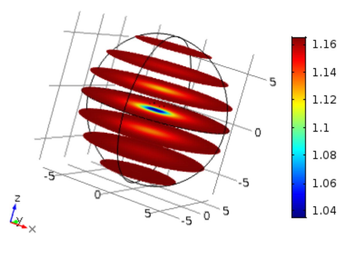
Figure 2: (a) A slice plot of the eigenfield inside a sphere, containing 8 small spherical inclusions, computed using the method of finite elements in COMSOL on a mesh with 1477957 elements. Contour plot of the eigenfield along the planes (b) x3=−0.5x_{3}=-0.5 and (d) x3=0.5x_{3}=0.5 based on the computations from COMSOL. The contour plot of the eigenfield on the planes (c) x3=−0.5x_{3}=-0.5 and (e) x3=0.5x_{3}=0.5 computed using the asymptotic approximation (7). The average absolute error between the computations in (b) and (c) is 2.1×10−32.1\times 10^{-3}, whereas between (d) and (e) it is 3.3×10−33.3\times 10^{-3}.
Refer to caption
Refer to caption
Refer to caption
Refer to caption
Refer to caption
Figure 3: (a) The cloud of 64 small inclusions contained in the cube (0,2)3(0,2)^{3}. (b)–(e) The asymptotic approximation for eigenfield corresponding to the first eigenvalue in the ball of radius 7, centred at the origin, and containing the cloud of inclusions. We show the cross-sectional plots on the planes (b) x3=0.25x_{3}=0.25, (c) x3=0.75x_{3}=0.75, (d) x3=1.25x_{3}=1.25 and (e) x3=1.75x_{3}=1.75.

For the purpose of illustration, in Fig. 2 we show the analytical asymptotic approximation versus the finite element simulation produced for a cluster of 8 Dirichlet-type inclusions on several cross-sections. The first eigenfunction in the overall three-dimensional domain with the cluster of inclusions is shown on Fig. 2.

The amount of memory required to run finite element computations increases substantially when the number NN of inclusions becomes large. For example, in 3-dimensions, with N=64N=64 inclusions in a cluster COMSOL fails due to lack of memory on a standard 16GB workstation. On the other hand, the proposed asymptotic algorithm remains robust and efficient with the results shown in Figure 3. The positions and the radii of inclusions are arbitrary, subject to constraints outlined earlier. In addition to the 3-dimensional illustration in Figure 3, we also show several cross-sectional plots in Figures 3–3. The asymptotic approximations are uniform and take into account mutual interaction between the inclusions with the cluster.

The structure of the article is as follows. In section 2 we formally introduce model problems necessary to compute the approximations (7) and (10). Formal asymptotic derivations of (7) and (10) are then given in section 3. Solvability of the system (8) is proven in section 4. We provide the steps used to attain the remainder estimates (9) and (10) in section 5. and going further in section 6, the higher-order approximation for the first eigenvalue and corresponding eigenfunction are given along with the completion of the proof of Theorems 1 and 2. A comparison of the approximations of Theorems 1 and 2 are compared with those produced by the method of compound asymptotic expansions [29] in section 7. In section 8, we further demonstrate the effectiveness of the approach presented here, by comparing (10) with numerical computations of eigenvalues for solids containing non-periodic clusters produced in COMSOL. In section 9, we discuss the homogenised problem obtained from the algebraic system (8) in the limit as the number of inclusions within the cluster grow. Finally in the Appendix, we present technical steps of the derivation to a higher order approximation of the first eigenvalue and corresponding eigenfunction given in section 6.

2 Model problems

We now introduce solutions to model problems that are necessary in constructing the asymptotic approximations for λN\lambda_{N} and uNu_{N}.

  1. 1.

    The Neumann function in Ω\Omega. Here, 𝒢{\cal G} denotes the Neumann function in Ω\Omega, which is a solution of

    Δ𝐱​𝒢​(𝐱,𝐲)+δ⁡(𝐱−𝐲)−1|Ω|=0,𝐱∈Ω,\Delta_{{\bf x}}{\cal G}({\bf x},{\bf y})+\delta({\bf x}-{\bf y})-\frac{1}{|\Omega|}=0\;,\quad{\bf x}\in\Omega\;, (11)
    ∂𝒢∂n𝐱​(𝐱,𝐲)=0,𝐱∈∂Ω.\frac{\partial{\cal G}}{\partial n_{\bf x}}({\bf x},{\bf y})=0\;,\quad{\bf x}\in\partial\Omega\;. (12)

    This definition of 𝒢{\cal G} is also supplied with the orthogonality condition

    ∫Ω𝒢⁡(𝐱,𝐲)​𝑑𝐱=0,\int_{\Omega}{\cal G}({\bf x},{\bf y})d{\bf x}=0\;,

    which implies the symmetry of 𝒢{\cal G}:

    𝒢⁡(𝐱,𝐲)=𝒢⁡(𝐲,𝐱),𝐱,𝐲∈Ω.{\cal G}({\bf x},{\bf y})={\cal G}({\bf y},{\bf x}),\quad{\bf x},{\bf y}\in\Omega\;.

    We also introduce the regular part ℋ{\cal H} of the Neumann function as

    ℋ⁡(𝐱,𝐲)=14​π​|𝐱−𝐲|−𝒢⁡(𝐱,𝐲).{\cal H}({\bf x},{\bf y})=\frac{1}{4\pi|{\bf x}-{\bf y}|}-{\cal G}({\bf x},{\bf y})\;.
  2. 2.

    Capacitary potential for the inclusion ωε(j)\omega_{\varepsilon}^{(j)}. The capacitary potentials Pε(j)P^{(j)}_{\varepsilon}, 1≤j≤N1\leq j\leq N, are used to construct boundary layers in the exterior of the small inclusions. The function Pε(j)P^{(j)}_{\varepsilon} solves

    Δ​Pε(j)​(𝐱)=0,𝐱∈ℝ3\ωε(j)¯,\Delta P_{\varepsilon}^{(j)}({\bf x})=0\;,\quad{\bf x}\in\mathbb{R}^{3}\backslash\overline{\omega^{(j)}_{\varepsilon}}\;,
    Pε(j)​(𝐱)=1,𝐱∈∂ωε(j),P_{\varepsilon}^{(j)}({\bf x})=1\;,\quad{\bf x}\in\partial\omega_{\varepsilon}^{(j)}\;,
    Pε(j)​(𝐱)→0, as ​|𝐱|→∞.P_{\varepsilon}^{(j)}({\bf x})\to 0\;,\quad\text{ as }|{\bf x}|\to\infty\;.

    The behaviour of the capacitary potential far from the inclusion ωε(j)\omega^{(j)}_{\varepsilon} is characterised by the capacity of this set, defined as

    cap​(ωε(j))=∫ℝ3\ωε(j)¯|∇Pε(j)​(𝐱)|2​𝑑𝐱.\text{cap}(\omega^{(j)}_{\varepsilon})=\int_{\mathbb{R}^{3}\backslash\overline{\omega^{(j)}_{\varepsilon}}}|\nabla P_{\varepsilon}^{(j)}({\bf x})|^{2}d{\bf x}\;.
    Lemma 1

    ((see [20])) For |𝐱−𝐎(j)|>2​ε|{\bf x}-{\bf O}^{(j)}|>2\varepsilon, the capacitary potential admits the asymptotic representation

    Pε(j)​(𝐱)=cap​(ωε(j))4​π​|𝐱−𝐎(j)|+O⁡(ε2|𝐱−𝐎(j)|2).P^{(j)}_{\varepsilon}({\bf x})=\frac{\text{\emph{cap}}(\omega^{(j)}_{\varepsilon})}{4\pi|{\bf x}-{\bf O}^{(j)}|}+O\Big(\frac{\varepsilon^{2}}{|{\bf x}-{\bf O}^{(j)}|^{2}}\Big)\;.

3 Formal asymptotic algorithm

We now derive formal asymptotics for the first eigenvalue λN\lambda_{N} and corresponding eigenfunction uNu_{N}.

First we state the asymptotic approximation for the first eigenvalue of the Laplacian in ΩN\Omega_{N}:

Lemma 2

The formal approximation to the first eigenvalue of Δ\Delta in ΩN\Omega_{N} is given by

λN=ΛN+λR,N,\displaystyle\lambda_{N}=\Lambda_{N}+\lambda_{R,N}\;, (13)

where

ΛN=−1|Ω|∑j=1NCjcap(ωε(j)),\Lambda_{N}=-\frac{1}{|\Omega|}\sum^{N}_{j=1}{C_{j}\text{\emph{cap}}(\omega^{(j)}_{\varepsilon})}\;, (14)

CjC_{j}, 1≤j≤N1\leq j\leq N, satisfy the algebraic system

0\displaystyle 0 =\displaystyle= 1+Ck​(1−cap​(ωε(k))​{ℋ⁡(𝐎(k),𝐎(k))−ΓΩ(k)})\displaystyle 1+C_{k}(1-\text{\emph{cap}}(\omega^{(k)}_{\varepsilon})\{{\cal H}({\bf O}^{(k)},{\bf O}^{(k)})-\Gamma_{\Omega}^{(k)}\}) (15)
+∑j≠k1≤j≤NCjcap(ωε(j)){𝒢(𝐎(k),𝐎(j))+ΓΩ(j)},1≤k≤N,\displaystyle+\sum_{\begin{subarray}{c}j\neq k\\ 1\leq j\leq N\end{subarray}}{C_{j}\text{\emph{cap}}(\omega^{(j)}_{\varepsilon})}\{{\cal G}({\bf O}^{(k)},{\bf O}^{(j)})+\Gamma_{\Omega}^{(j)}\}\;,\quad 1\leq k\leq N\;,

and λR,N\lambda_{R,N} is the remainder of the approximation.

We present the formal scheme leading to the preceding approximation and of the first eigenfunction uNu_{N} contained in the next lemma.

Lemma 3

The formal approximation of the eigenfunction uNu_{N} of problem (2)(\ref{uN1})–(4)(\ref{uN3}) has the form

uN​(𝐱)=U⁡(𝐱)+RN​(𝐱),\displaystyle u_{N}({\bf x})=U({\bf x})+R_{N}({\bf x})\;, (16)

where

U⁡(𝐱)\displaystyle U({\bf x}) =\displaystyle= 1+∑j=1NCj​ΓΩ(j)​cap​(ωε(j))\displaystyle 1+\sum_{j=1}^{N}{C_{j}\Gamma^{(j)}_{\Omega}\text{\emph{cap}}(\omega^{(j)}_{\varepsilon})} (17)
+∑j=1NCj{Pε(j)(𝐱)−cap(ωε(j))ℋ(𝐱,𝐎(j))},\displaystyle+\sum^{N}_{j=1}C_{j}\{P^{(j)}_{\varepsilon}({\bf x})-\text{\emph{cap}}(\omega^{(j)}_{\varepsilon}){\cal H}({\bf x},{\bf O}^{(j)})\}\;,

the coefficients CjC_{j} satisfy the linear algebraic system (15)(\ref{form_sys}) and the function UU, defined according to (17)(\ref{uN=U+RN}), satisfies the problem

Δ​U​(𝐱)+ΛN​U​(𝐱)=fN​(𝐱),𝐱∈ΩN,\displaystyle\Delta U({\bf x})+\Lambda_{N}U({\bf x})=f_{N}({\bf x})\;,\quad{\bf x}\in\Omega_{N}\;,
∂U⁡(𝐱)∂n=ψ⁡(𝐱),𝐱∈∂Ω,\displaystyle\frac{\partial U({\bf x})}{\partial n}=\psi({\bf x})\;,\quad{\bf x}\in\partial\Omega\;,
U⁡(𝐱)=ϕk​(𝐱),𝐱∈∂ωε(k),1≤k≤N,\displaystyle U({\bf x})=\phi_{k}({\bf x})\;,\quad{\bf x}\in\partial\omega_{\varepsilon}^{(k)},1\leq k\leq N\;,

where

|fN​(𝐱)|=O⁡(ε2​d−3​(d−3+∑j=1N|Cj||𝐱−𝐎(j)|)),𝐱∈ΩN,\displaystyle|f_{N}({\bf x})|=O\Big(\varepsilon^{2}d^{-3}\Big(d^{-3}+\sum_{j=1}^{N}\frac{|C_{j}|}{|{\bf x}-{\bf O}^{(j)}|}\Big)\Big)\;,\quad{\bf x}\in\Omega_{N}\;,
|ψ⁡(𝐱)|=O⁡(∑j=1Nε2​|Cj||𝐱−𝐎(j)|3),𝐱∈∂Ω,\displaystyle|\psi({\bf x})|=O\Big(\sum_{j=1}^{N}\frac{\varepsilon^{2}|C_{j}|}{|{\bf x}-{\bf O}^{(j)}|^{3}}\Big)\;,\quad{\bf x}\in\partial\Omega\;,
|ϕk​(𝐱)|=O⁡(ε2​(d−3+∑j≠k1≤j≤N|Cj||𝐎(k)−𝐎(j)|2)),𝐱∈∂ωε(j),1≤k≤N.\displaystyle|\phi_{k}({\bf x})|=O\Big(\varepsilon^{2}\Big(d^{-3}+\sum_{\begin{subarray}{c}j\neq k\\ 1\leq j\leq N\end{subarray}}\frac{|C_{j}|}{|{\bf O}^{(k)}-{\bf O}^{(j)}|^{2}}\Big)\Big)\;,{\bf x}\in\partial\omega_{\varepsilon}^{(j)}\;,1\leq k\leq N\;.

Proof of Lemmas 2 and 3. Let

U⁡(𝐱)\displaystyle U({\bf x}) =\displaystyle= 1+∑j=1NCj​Pε(j)​(𝐱)+u1​(𝐱).\displaystyle 1+\sum_{j=1}^{N}C_{j}P_{\varepsilon}^{(j)}({\bf x})+u_{1}({\bf x})\;. (18)

It is assumed the remainders RN​(𝐱)R_{N}({\bf x}) and λR,N\lambda_{R,N} in (16) and (13) are of the order O⁡(ε2​d−6)O(\varepsilon^{2}d^{-6}). In addition, we will show

u1​(𝐱)=O⁡(ε​d−3) and ΛN=O⁡(ε​d−3).\displaystyle u_{1}({\bf x})=O(\varepsilon d^{-3})\quad\text{ and }\quad\Lambda_{N}=O(\varepsilon d^{-3})\;.

The governing equation in ΩN\Omega_{N}. According to (18), it holds that

0=Δ​U​(𝐱)+ΛN​U​(𝐱)\displaystyle 0=\Delta U({\bf x})+\Lambda_{N}U({\bf x})
=\displaystyle= Δ⁡(1+∑j=1NCj​Pε(j)​(𝐱)+u1​(𝐱))+ΛN​(1+∑j=1NCj​Pε(j)​(𝐱)+u1​(𝐱))\displaystyle\Delta\Big(1+\sum_{j=1}^{N}C_{j}P_{\varepsilon}^{(j)}({\bf x})+u_{1}({\bf x})\Big)+\Lambda_{N}\Big(1+\sum_{j=1}^{N}C_{j}P_{\varepsilon}^{(j)}({\bf x})+u_{1}({\bf x})\Big)
for ​𝐱∈ΩN.\displaystyle\text{ for }{\bf x}\in\Omega_{N}\;.

Since the capacitary potentials are harmonic, this implies in ΩN\Omega_{N} that

Δ​U​(𝐱)+ΛN​U​(𝐱)=Δ​u1​(𝐱)+ΛN​(1+∑j=1NCj​Pε(j)​(𝐱)+u1​(𝐱)).\displaystyle\Delta U({\bf x})+\Lambda_{N}U({\bf x})=\Delta u_{1}({\bf x})+\Lambda_{N}\Big(1+\sum_{j=1}^{N}C_{j}P_{\varepsilon}^{(j)}({\bf x})+u_{1}({\bf x})\Big)\;. (19)

For 𝐱∈ΩN{\bf x}\in\Omega_{N}, one can write

Pε(j)​(𝐱)=cap​(ωε(j))4​π​|𝐱−𝐎(j)|+O⁡(ε2|𝐱−𝐎(j)|2),P^{(j)}_{\varepsilon}({\bf x})=\frac{\text{cap}(\omega_{\varepsilon}^{(j)})}{4\pi|{\bf x}-{\bf O}^{(j)}|}+O\Big(\frac{\varepsilon^{2}}{|{\bf x}-{\bf O}^{(j)}|^{2}}\Big)\;,

(see [29, 30]). As a result, returning to (19) we then have

Δ​U​(𝐱)+ΛN​U​(𝐱)\displaystyle\Delta U({\bf x})+\Lambda_{N}U({\bf x})
=Δ​u1​(𝐱)+ΛN+O⁡(ε2​d−6)+O⁡(ε2​d−3​∑j=1N|Cj||𝐱−𝐎(j)|).\displaystyle=\Delta u_{1}({\bf x})+\Lambda_{N}+O(\varepsilon^{2}d^{-6})+O\Big(\varepsilon^{2}d^{-3}\sum_{j=1}^{N}\frac{|C_{j}|}{|{\bf x}-{\bf O}^{(j)}|}\Big)\;. (20)

Exterior boundary condition. Next we consider the normal derivative of U⁡(𝐱)U({\bf x}) on ∂Ω\partial\Omega. We have

∂U⁡(𝐱)∂n=∂∂n​{1+∑j=1NCj​Pε(j)​(𝐱)+u1​(𝐱)},𝐱∈∂Ω.\frac{\partial U({\bf x})}{\partial n}=\frac{\partial}{\partial n}\Big\{1+\sum_{j=1}^{N}C_{j}P_{\varepsilon}^{(j)}({\bf x})+u_{1}({\bf x})\Big\}\quad\;,{\bf x}\in\partial\Omega\;.

Using Lemma 1, this can be updated to

∂U⁡(𝐱)∂n=∂∂n​{∑j=1NCj​cap​(ωε(j))4​π​|𝐱−𝐎(j)|+u1​(𝐱)}+O⁡(∑j=1Nε2​|Cj||𝐱−𝐎(j)|3),\displaystyle\frac{\partial U({\bf x})}{\partial n}=\frac{\partial}{\partial n}\Big\{\sum_{j=1}^{N}\frac{C_{j}\text{cap}(\omega_{\varepsilon}^{(j)})}{4\pi|{\bf x}-{\bf O}^{(j)}|}+u_{1}({\bf x})\Big\}+O\Big(\sum_{j=1}^{N}\frac{\varepsilon^{2}|C_{j}|}{|{\bf x}-{\bf O}^{(j)}|^{3}}\Big)\;, (21)

for 𝐱∈∂Ω{\bf x}\in\partial\Omega.

The terms u1u_{1} and ΛN\Lambda_{N}. Consulting (20) and (21), we set

Δ​u1​(𝐱)=−ΛN,𝐱∈Ω,\Delta u_{1}({\bf x})=-\Lambda_{N}\;,\quad{\bf x}\in\Omega\;, (22)
∂u1​(𝐱)∂n=−∂∂n​{∑j=1NCj​cap​(ωε(j))4​π​|𝐱−𝐎(j)|},𝐱∈∂Ω,\frac{\partial u_{1}({\bf x})}{\partial n}=-\frac{\partial}{\partial n}\Big\{\sum^{N}_{j=1}\frac{C_{j}\text{cap}(\omega^{(j)}_{\varepsilon})}{4\pi|{\bf x}-{\bf O}^{(j)}|}\Big\}\;,\quad{\bf x}\in\partial\Omega\;, (23)

and we prescribe that

∫Ωu1​(𝐱)​𝑑𝐱=0.\int_{\Omega}u_{1}({\bf x})d{\bf x}=0\;. (24)

Note that according to this problem, the term Λ1\Lambda_{1} can be computed using Green’s identity in Ω\Omega to give

−|Ω|​ΛN\displaystyle-|\Omega|\Lambda_{N} =\displaystyle= ∫ΩΔ​uN​(𝐱)​𝑑𝐱=∫∂Ω∂uN∂n​(𝐱)​d​S𝐱\displaystyle\int_{\Omega}\Delta u_{N}({\bf x})d{\bf x}=\int_{\partial\Omega}\frac{\partial u_{N}}{\partial n}({\bf x})dS_{{\bf x}}
=\displaystyle= −∫∂Ω∂∂n𝐱{∑j=1NCj​cap​(ωε(j))4​π​|𝐱−𝐎(j)|}dS𝐱\displaystyle-\int_{\partial\Omega}\frac{\partial}{\partial n_{{\bf x}}}\Big\{\sum^{N}_{j=1}\frac{C_{j}\text{cap}(\omega^{(j)}_{\varepsilon})}{4\pi|{\bf x}-{\bf O}^{(j)}|}\Big\}dS_{{\bf x}}
=\displaystyle= ∑j=1NCj​cap​(ωε(j)).\displaystyle\sum^{N}_{j=1}{C_{j}\text{cap}(\omega^{(j)}_{\varepsilon})}\;.

Thus, from this we prove (14) of Lemma 2.

In addition, u1u_{1} can be constructed in the form

u1(𝐱)=−∑j=1NCjcap(ωε(j)){ℋ(𝐱,𝐎(j))−ΓΩ(j)},u_{1}({\bf x})=-\sum_{j=1}^{N}C_{j}\text{cap}(\omega^{(j)}_{\varepsilon})\Big\{{\cal H}({\bf x},{\bf O}^{(j)})-\Gamma_{\Omega}^{(j)}\Big\}\;, (25)

with ΓΩ(k)\Gamma_{\Omega}^{(k)} specified in (5). It can be checked this satisfies (22)–(24).

Interior boundary conditions on small inclusions. Taking the trace of U⁡(𝐱)U({\bf x}) on the boundary of ∂ωε(k)\partial\omega^{(k)}_{\varepsilon}, 1≤k≤N1\leq k\leq N, and using the definition of the capacitary potentials gives

U⁡(𝐱)\displaystyle U({\bf x}) =\displaystyle= 1+Ck+∑j≠k1≤j≤NCj​Pε(j)​(𝐱)+u1​(𝐱).\displaystyle 1+C_{k}+\sum_{\begin{subarray}{c}j\neq k\\ 1\leq j\leq N\end{subarray}}C_{j}P_{\varepsilon}^{(j)}({\bf x})+u_{1}({\bf x})\;.

Next, Taylor’s expansion about 𝐱=𝐎(k){\bf x}={\bf O}^{(k)} and Lemma 1 can be employed in the above condition to obtain

U⁡(𝐱)\displaystyle U({\bf x}) =\displaystyle= 1+Ck+∑j≠k1≤j≤NCj​cap​(ωε(j))4​π​|𝐎(k)−𝐎(j)|+u1​(𝐎(k))\displaystyle 1+C_{k}+\sum_{\begin{subarray}{c}j\neq k\\ 1\leq j\leq N\end{subarray}}\frac{C_{j}\text{cap}(\omega^{(j)}_{\varepsilon})}{4\pi|{\bf O}^{(k)}-{\bf O}^{(j)}|}+u_{1}({\bf O}^{(k)})
+O⁡(ε2​d−3)+O⁡(∑j≠k1≤j≤Nε2​|Cj||𝐎(k)−𝐎(j)|2)\displaystyle+O(\varepsilon^{2}d^{-3})+O\Big(\sum_{\begin{subarray}{c}j\neq k\\ 1\leq j\leq N\end{subarray}}\frac{\varepsilon^{2}|C_{j}|}{|{\bf O}^{(k)}-{\bf O}^{(j)}|^{2}}\Big)

for 𝐱∈∂ωε(k){\bf x}\in\partial\omega^{(k)}_{\varepsilon}, 1≤k≤N1\leq k\leq N. According to (25), this is equivalent to

U⁡(𝐱)\displaystyle U({\bf x}) =\displaystyle= 1+Ck​(1−cap​(ωε(k))​{ℋ⁡(𝐎(k),𝐎(k))−ΓΩ(k)})\displaystyle 1+C_{k}(1-\text{cap}(\omega_{\varepsilon}^{(k)})\{{\cal H}({\bf O}^{(k)},{\bf O}^{(k)})-\Gamma_{\Omega}^{(k)}\}) (26)
+∑j≠k1≤j≤NCjcap(ωε(j)){𝒢(𝐎(k),𝐎(j))+ΓΩ(j)}\displaystyle+\sum_{\begin{subarray}{c}j\neq k\\ 1\leq j\leq N\end{subarray}}{C_{j}\text{cap}(\omega^{(j)}_{\varepsilon})}\{{\cal G}({\bf O}^{(k)},{\bf O}^{(j)})+\Gamma_{\Omega}^{(j)}\}
+O⁡(ε2​d−3)+O⁡(∑j≠k1≤j≤Nε2​|Cj||𝐎(k)−𝐎(j)|2).\displaystyle+O(\varepsilon^{2}d^{-3})+O\Big(\sum_{\begin{subarray}{c}j\neq k\\ 1\leq j\leq N\end{subarray}}\frac{\varepsilon^{2}|C_{j}|}{|{\bf O}^{(k)}-{\bf O}^{(j)}|^{2}}\Big)\;.

We then set up a system of algebraic equations with respect to CkC_{k}, 1≤k≤N1\leq k\leq N, as

0\displaystyle 0 =\displaystyle= 1+Ck​(1−cap​(ωε(k))​{ℋ⁡(𝐎(k),𝐎(k))−ΓΩ(k)})\displaystyle 1+C_{k}(1-\text{{cap}}(\omega^{(k)}_{\varepsilon})\{{\cal H}({\bf O}^{(k)},{\bf O}^{(k)})-\Gamma_{\Omega}^{(k)}\}) (27)
+∑j≠k1≤j≤NCjcap(ωε(j)){𝒢(𝐎(k),𝐎(j))+ΓΩ(j)},\displaystyle+\sum_{\begin{subarray}{c}j\neq k\\ 1\leq j\leq N\end{subarray}}{C_{j}\text{cap}(\omega^{(j)}_{\varepsilon})}\{{\cal G}({\bf O}^{(k)},{\bf O}^{(j)})+\Gamma_{\Omega}^{(j)}\}\;,

to remove the leading order term in (26). The preceding together with (13) and (14) prove Lemma 2.

The problem for UU. As a result of equations (20), (22), we have that UU satisfies

Δ​U​(𝐱)+ΛN​U​(𝐱)=O⁡(ε2​d−6)+O⁡(ε2​d−3​∑j=1N|Cj||𝐱−𝐎(j)|),𝐱∈ΩN.\displaystyle\Delta U({\bf x})+\Lambda_{N}U({\bf x})=O(\varepsilon^{2}d^{-6})+O\Big(\varepsilon^{2}d^{-3}\sum_{j=1}^{N}\frac{|C_{j}|}{|{\bf x}-{\bf O}^{(j)}|}\Big)\;,\quad{\bf x}\in\Omega_{N}\;.
(28)

On the exterior boundary, owing to (21) and (23) we obtain

∂U⁡(𝐱)∂n=O⁡(∑j=1Nε2​|Cj||𝐱−𝐎(j)|3),𝐱∈∂Ω.\displaystyle\frac{\partial U({\bf x})}{\partial n}=O\Big(\sum_{j=1}^{N}\frac{\varepsilon^{2}|C_{j}|}{|{\bf x}-{\bf O}^{(j)}|^{3}}\Big)\;,\quad{\bf x}\in\partial\Omega\;. (29)

The algebraic system (27) with (26) provide on the interior boundaries

U⁡(𝐱)\displaystyle U({\bf x}) =\displaystyle= O⁡(ε2​d−3)+O⁡(∑j≠k1≤j≤Nε2​|Cj||𝐎(k)−𝐎(j)|2)\displaystyle O(\varepsilon^{2}d^{-3})+O\Big(\sum_{\begin{subarray}{c}j\neq k\\ 1\leq j\leq N\end{subarray}}\frac{\varepsilon^{2}|C_{j}|}{|{\bf O}^{(k)}-{\bf O}^{(j)}|^{2}}\Big) (30)

for 𝐱∈∂ωε(k){\bf x}\in\partial\omega_{\varepsilon}^{(k)}, 1≤k≤N1\leq k\leq N.

By combining (16), (18), (25), (27) and (28)–(30), we arrive at the proof of Lemma 3. □\Box

4 The algebraic system and its solvability

In this section, it will be shown that the algebraic system (27) identified in the previous sections is solvable. Here we rewrite the system (15) as

0\displaystyle 0 =\displaystyle= 1+Ck​(1−cap​(ωε(k))​ℋ​(𝐎(k),𝐎(k)))\displaystyle 1+C_{k}(1-\text{cap}(\omega_{\varepsilon}^{(k)}){\cal H}({\bf O}^{(k)},{\bf O}^{(k)}))
+∑j≠k1≤j≤NCjcap(ωε(j))g(𝐎(k),𝐎(j))−ΓΩ(k)∑j=1NCjcap(ωε(j)),\displaystyle+\sum_{\begin{subarray}{c}j\neq k\\ 1\leq j\leq N\end{subarray}}{C_{j}\text{{cap}}(\omega^{(j)}_{\varepsilon})}g({\bf O}^{(k)},{\bf O}^{(j)})-\Gamma_{\Omega}^{(k)}\sum_{j=1}^{N}C_{j}\text{cap}(\omega_{\varepsilon}^{(j)})\;,

where

g⁡(𝐱,𝐲)=𝒢⁡(𝐱,𝐲)+ΓΩ​(𝐲)+ΓΩ​(𝐱),g({\bf x},{\bf y})={\cal G}({\bf x},{\bf y})+\Gamma_{\Omega}({\bf y})+\Gamma_{\Omega}({\bf x})\;, (31)

and

ΓΩ​(𝐱)=1|Ω|​∫Ωd​𝐳4​π​|𝐳−𝐱|.\Gamma_{\Omega}({\bf x})=\frac{1}{|\Omega|}\int_{\Omega}\frac{d{\bf z}}{4\pi|{\bf z}-{\bf x}|}\;.

This system can then be written in matrix form as:

−𝐄=(𝐈−𝐇𝐃+𝐆𝐃−𝚪​𝐃)​𝐂,-{\bf E}=({\bf I}-{\bf H}{\bf D}+{\bf G}{\bf D}-\mbox{\boldmath${\Gamma}$}{\bf D}){\bf C}\;, (32)

where 𝐈{\bf I} is the N×NN\times N identity matrix,

𝐂=(C1,…,CN)T,𝐄=∑j=1N𝐞j(N),{\bf C}=(C_{1},\dots,C_{N})^{T}\;,\quad{\bf E}=\sum_{j=1}^{N}{\bf e}^{(N)}_{j}\;,

and 𝐞i(N)=[δi​j]j=1N{\bf e}^{(N)}_{i}=[\delta_{ij}]_{j=1}^{N}. In addition 𝐆=[Gi​j]i,j=1N{\bf G}=[G_{ij}]_{i,j=1}^{N} with

Gi​j={g⁡(𝐎(i),𝐎(j)), for ​i≠j,0,otherwise,G_{ij}=\left\{\begin{array}[]{ll}\displaystyle{g({\bf O}^{(i)},{\bf O}^{(j)})}\;,&\quad\text{ for }i\neq j\;,\\ \\ 0\;,&\quad\text{otherwise,}\end{array}\right.

and

𝐇=diag1≤j≤N​{ℋ⁡(𝐎(j),𝐎(j))},{\bf H}=\text{diag}_{1\leq j\leq N}\{{\cal H}({\bf O}^{(j)},{\bf O}^{(j)})\}\;,
𝚪=[ΓΩ(j)]i,j=1N,𝐃=diag1≤j≤N​{cap​(ωε(j))}.\mbox{\boldmath${\Gamma}$}=[\Gamma_{\Omega}^{(j)}]_{i,j=1}^{N}\;,\quad{\bf D}=\text{diag}_{1\leq j\leq N}\{\text{cap}(\omega^{(j)}_{\varepsilon})\}\;.

Solvability of the algebraic systems

We consider the system (32), whose rows can be written as in (27), and here we show the invertibility of the N×NN\times N matrix 𝐈+(𝐆−𝐇−𝚪)​𝐃{\bf I}+({\bf G}-{\bf H}-\mbox{\boldmath${\Gamma}$}){\bf D}.

Taking the scalar product of (32) with 𝐃𝐂{\bf D}{\bf C} one obtains

−⟨𝐃𝐂,𝐄⟩\displaystyle-\langle{\bf D}{\bf C},{\bf E}\rangle =\displaystyle= ⟨𝐃𝐂,𝐂⟩+⟨𝐃𝐂,𝐆𝐃𝐂⟩\displaystyle\langle{\bf D}{\bf C},{\bf C}\rangle+\langle{\bf D}{\bf C},{\bf G}{\bf D}{\bf C}\rangle (33)
−⟨𝐃𝐂,𝐇𝐃𝐂⟩−⟨𝐃𝐂,𝚪​𝐃𝐂⟩.\displaystyle-\langle{\bf D}{\bf C},{\bf H}{\bf D}{\bf C}\rangle-\langle{\bf D}{\bf C},\mbox{\boldmath${\Gamma}$}{\bf D}{\bf C}\rangle\;.

In proving the solvability of (27), we need the following estimates:

Lemma 4

The estimates

|⟨𝐃𝐂,𝐇𝐃𝐂⟩|\displaystyle|\langle{\bf D}{\bf C},{\bf H}{\bf D}{\bf C}\rangle| ≤\displaystyle\leq Const ​ε​⟨𝐂,𝐃𝐂⟩,\displaystyle\text{\emph{Const} }\varepsilon\,\langle{\bf C},{\bf D}{\bf C}\rangle\;, (34)
|⟨𝐃𝐂,𝚪​𝐃𝐂⟩|\displaystyle|\langle{\bf D}{\bf C},\mbox{\boldmath${\Gamma}$}{\bf D}{\bf C}\rangle| ≤\displaystyle\leq Const ​ε​d−3​⟨𝐂,𝐃𝐂⟩\displaystyle\text{\emph{Const} }\varepsilon\,d^{-3}\langle{\bf C},{\bf D}{\bf C}\rangle (35)

and

⟨𝐃𝐂,𝐆𝐃𝐂⟩≥−Const ​d−1​⟨𝐃𝐂,𝐃𝐂⟩.\langle{\bf D}{\bf C},{\bf G}{\bf D}{\bf C}\rangle\geq-\text{\emph{Const} }d^{-1}\langle{\bf D}{\bf C},{\bf D}{\bf C}\rangle\;. (36)

hold.

Proof of (34)(\ref{CHC}) and (35)(\ref{CGC}). Since the regular part ℋ{\cal H} is bounded in ω\omega, one has that

|⟨𝐃𝐂,𝐇𝐃𝐂⟩|\displaystyle|\langle{\bf D}{\bf C},{\bf H}{\bf D}{\bf C}\rangle| =\displaystyle= |∑k=1N(Ck​cap​(ωε(k)))2​ℋ​(𝐎(k),𝐎(k))|\displaystyle\Big|\sum_{k=1}^{N}(C_{k}\text{cap}(\omega_{\varepsilon}^{(k)}))^{2}{\cal H}({\bf O}^{(k)},{\bf O}^{(k)})\Big|
≤\displaystyle\leq Const ​ε​⟨𝐂,𝐃𝐂⟩,\displaystyle\text{Const }\varepsilon\,\langle{\bf C},{\bf D}{\bf C}\rangle\;,

which is (34). In addition, using (5) gives

|⟨𝐃𝐂,𝚪​𝐃𝐂⟩|\displaystyle|\langle{\bf D}{\bf C},\mbox{\boldmath${\Gamma}$}{\bf D}{\bf C}\rangle| ≤\displaystyle\leq ∑k=1N∑j=1N|Ck​Cj​cap​(ωε(k))​cap​(ωε(j))​ΓΩ(k)|\displaystyle\sum_{k=1}^{N}\sum_{j=1}^{N}|C_{k}C_{j}\text{cap}(\omega_{\varepsilon}^{(k)})\text{cap}(\omega_{\varepsilon}^{(j)})\Gamma_{\Omega}^{(k)}|
≤\displaystyle\leq Const ​∑k=1N∑j=1N|Ck​Cj​cap​(ωε(k))​cap​(ωε(j))|.\displaystyle\text{Const }\sum_{k=1}^{N}\sum_{j=1}^{N}|C_{k}C_{j}\text{cap}(\omega_{\varepsilon}^{(k)})\text{cap}(\omega_{\varepsilon}^{(j)})|\;.

The Cauchy inequality then implies

|⟨𝐃𝐂,𝚪​𝐃𝐂⟩|\displaystyle|\langle{\bf D}{\bf C},\mbox{\boldmath${\Gamma}$}{\bf D}{\bf C}\rangle| ≤\displaystyle\leq Const ​⟨𝐃𝐂,𝐂⟩​∑k=1Ncap​(ωε(k))\displaystyle\text{Const }\langle{\bf D}{\bf C},{\bf C}\rangle\sum_{k=1}^{N}\text{cap}(\omega_{\varepsilon}^{(k)})
≤\displaystyle\leq Const ​ε​d−3​⟨𝐃𝐂,𝐂⟩,\displaystyle\text{Const }\varepsilon d^{-3}\langle{\bf D}{\bf C},{\bf C}\rangle\;,

proving (35).

Proof of (36)(\ref{import_ineq}). The term

⟨𝐃𝐂,𝐆𝐃𝐂⟩=∑k=1NCk​cap​(ωε(k))​∑j≠k1≤j≤Ng⁡(𝐎(k),𝐎(j))​Cj​cap​(ωε(j)).\langle{\bf D}{\bf C},{\bf G}{\bf D}{\bf C}\rangle=\sum_{k=1}^{N}C_{k}\text{cap}(\omega^{(k)}_{\varepsilon})\sum_{\begin{subarray}{c}j\neq k\\ 1\leq j\leq N\end{subarray}}{g({\bf O}^{(k)},{\bf O}^{(j)})}{C_{j}\text{cap}(\omega^{(j)}_{\varepsilon})}\;. (37)

According to (11) and (12) the function gg defined in (31) satisfies

Δ𝐗​g​(𝐗,𝐘)+δ⁡(𝐗−𝐘)=0,𝐗,𝐘∈Ω,\Delta_{{\bf X}}g({\bf X},{\bf Y})+\delta({\bf X}-{\bf Y})=0\;,\quad{\bf X},{\bf Y}\in\Omega\;, (38)
∂g∂n𝐗​(𝐗,𝐘)=∂ΓΩ∂n𝐗​(𝐗),𝐗∈∂Ω,𝐘∈Ω.\frac{\partial g}{\partial n_{\bf X}}({\bf X},{\bf Y})=\frac{\partial\Gamma_{\Omega}}{\partial n_{\bf X}}({\bf X})\;,\quad{\bf X}\in\partial\Omega\;,{\bf Y}\in\Omega\;.

It is also true from (31) that

g⁡(𝐗,𝐘)=g⁡(𝐘,𝐗),𝐗≠𝐘.g({\bf X},{\bf Y})=g({\bf Y},{\bf X}),\quad{\bf X}\neq{\bf Y}\;.

As a result, application of Green’s formula to g⁡(𝐙,𝐗)g({\bf Z},{\bf X}) and g⁡(𝐙,𝐘)g({\bf Z},{\bf Y}) shows that this function satisfies the orthogonality condition:

∫∂Ωg⁡(𝐙,𝐘)​∂ΓΩ∂n𝐗​(𝐙)​d​S𝐙=0.\int_{\partial\Omega}g({\bf Z},{\bf Y})\frac{\partial\Gamma_{\Omega}}{\partial n_{\bf X}}({\bf Z})dS_{{\bf Z}}=0\;. (39)

Here, (38) shows that gg is harmonic if 𝐗≠𝐘{\bf X}\neq{\bf Y}. Using this, (37) can be rewritten with the mean value theorem inside disjoint balls to give

⟨𝐃𝐂,𝐆𝐃𝐂⟩\displaystyle\langle{\bf D}{\bf C},{\bf G}{\bf D}{\bf C}\rangle (40)
=\displaystyle= 482π2​d6​∑k=1N∑j=1N∫B(k)∫B(j)Ck​cap​(ωε(k))​g​(𝐗,𝐘)​Cj​cap​(ωε(j))​𝑑𝐗​𝑑𝐘\displaystyle\frac{48^{2}}{\pi^{2}d^{6}}\sum_{k=1}^{N}\sum_{j=1}^{N}\int_{B^{(k)}}\int_{B^{(j)}}C_{k}\text{cap}(\omega^{(k)}_{\varepsilon}){g({\bf X},{\bf Y})}{C_{j}\text{cap}(\omega^{(j)}_{\varepsilon})}d{\bf X}d{\bf Y}
−48π​d3∑k=1N(Ckcap(ωε(k)))2∫B(k)g(𝐗,𝐎(k))d𝐗.\displaystyle-\frac{48}{\pi d^{3}}\sum_{k=1}^{N}(C_{k}\text{cap}(\omega_{\varepsilon}^{(k)}))^{2}\int_{B^{(k)}}g({\bf X},{\bf O}^{(k)})d{\bf X}\;.

where B(j)={𝐗:|𝐗−𝐎(j)|<d/4}B^{(j)}=\{{\bf X}:|{\bf X}-{\bf O}^{(j)}|<d/4\}.

Next the fact g⁡(𝐱,𝐎(k))=O⁡(|𝐗−𝐎(k)|−1)g({\bf x},{\bf O}^{(k)})=O(|{\bf X}-{\bf O}^{(k)}|^{-1}) allows for the estimate

∫B(k)g⁡(𝐗,𝐎(k))​𝑑𝐗≤Const ​d2.\int_{B^{(k)}}g({\bf X},{\bf O}^{(k)})d{\bf X}\leq\text{Const }d^{2}\;. (41)

The function

Θ⁡(𝐱)={Ck​cap​(ωε(k)),𝐱∈B(k)0otherwise,\Theta({\bf x})=\left\{\begin{array}[]{ll}C_{k}\text{cap}(\omega^{(k)}_{\varepsilon})\;,&\quad{\bf x}\in B^{(k)}\\ 0&\quad\text{otherwise},\end{array}\right.

can be employed to the double sum in (40) to yield:

∑k=1N∑j=1N∫B(k)∫B(j)Ck​cap​(ωε(k))​g​(𝐗,𝐘)​Cj​cap​(ωε(j))​𝑑𝐗​𝑑𝐘\displaystyle\sum_{k=1}^{N}\sum_{j=1}^{N}\int_{B^{(k)}}\int_{B^{(j)}}C_{k}\text{cap}(\omega^{(k)}_{\varepsilon}){g({\bf X},{\bf Y})}{C_{j}\text{cap}(\omega^{(j)}_{\varepsilon})}d{\bf X}d{\bf Y} (42)
=\displaystyle= ∫Ω∫ΩΘ⁡(𝐗)​g​(𝐗,𝐘)​Θ​(𝐘)​𝑑𝐗​𝑑𝐘.\displaystyle\int_{\Omega}\int_{\Omega}\Theta({\bf X})g({\bf X},{\bf Y})\Theta({\bf Y})d{\bf X}d{\bf Y}\;.

Next set

h⁡(𝐗)=∫Ωg⁡(𝐗,𝐘)​Θ​(𝐘)​𝑑𝐘.h({\bf X})=\int_{\Omega}g({\bf X},{\bf Y})\Theta({\bf Y})d{\bf Y}\;.

This function satisfies

Δ𝐱​h​(𝐗)=−Θ⁡(𝐗),𝐗∈Ω,\Delta_{\bf x}h({\bf X})=-\Theta({\bf X})\;,\quad{\bf X}\in\Omega\;, (43)
∂h∂n𝐗​(𝐗)=∂ΓΩ∂n𝐱​(𝐗)​∫ΩΘ⁡(𝐘)​𝑑𝐘.\frac{\partial h}{\partial n_{\bf X}}({\bf X})=\frac{\partial\Gamma_{\Omega}}{\partial n_{\bf x}}({\bf X})\int_{\Omega}\Theta({\bf Y})d{\bf Y}\;.

Note that owing to (39):

∫∂Ωh⁡(𝐗)​∂h∂n𝐗​(𝐗)​d​S𝐗=∫∂Ωh⁡(𝐗)​∂ΓΩ∂n𝐗​(𝐗)​d​S𝐗​∫ΩΘ⁡(𝐘)​𝑑𝐘=0.\int_{\partial\Omega}h({\bf X})\frac{\partial h}{\partial n_{\bf X}}({\bf X})dS_{\bf X}=\int_{\partial\Omega}h({\bf X})\frac{\partial\Gamma_{\Omega}}{\partial n_{\bf X}}({\bf X})dS_{\bf X}\int_{\Omega}\Theta({\bf Y})d{\bf Y}=0\;.

Thus, after integration by parts, one can show using this and (43) that

∫Ω∫ΩΘ⁡(𝐗)​g​(𝐗,𝐘)​Θ​(𝐘)​𝑑𝐗​𝑑𝐘=∫Ω|∇h​(𝐱)|2​𝑑𝐱≥0.\int_{\Omega}\int_{\Omega}\Theta({\bf X})g({\bf X},{\bf Y})\Theta({\bf Y})d{\bf X}d{\bf Y}=\int_{\Omega}|\nabla h({\bf x})|^{2}d{\bf x}\geq 0\;.

Then, this estimate, (37), (40), (41) and (42) prove (36), completing the proof. □\Box

Lemma 5

Let the small parameters ε\varepsilon and dd satisfy the inequality

ε<c​d3\varepsilon<c\,d^{3} (44)

where cc is a sufficiently small constant. Then the system (32)(\ref{sys1}) is solvable and the estimate

∑j=1NCj2≤Const ​d−3,\sum_{j=1}^{N}C_{j}^{2}\leq\text{\emph{Const }}d^{-3}\;, (45)

holds.

Proof. We start from (33), and use the Cauchy inequality to obtain

⟨𝐄,𝐃𝐄⟩1/2​⟨𝐂,𝐃𝐂⟩1/2\displaystyle\langle{\bf E},{\bf D}{\bf E}\rangle^{1/2}\langle{\bf C},{\bf D}{\bf C}\rangle^{1/2} ≥\displaystyle\geq ⟨𝐂,𝐃𝐂⟩+⟨𝐃𝐂,𝐆𝐃𝐂⟩\displaystyle\langle{\bf C},{\bf D}{\bf C}\rangle+\langle{\bf D}{\bf C},{\bf G}{\bf D}{\bf C}\rangle
−⟨𝐃𝐂,𝐇𝐃𝐂⟩−⟨𝐃𝐂,𝚪​𝐃𝐂⟩\displaystyle-\langle{\bf D}{\bf C},{\bf H}{\bf D}{\bf C}\rangle-\langle{\bf D}{\bf C},\mbox{\boldmath${\Gamma}$}{\bf D}{\bf C}\rangle

Now from Lemma 4, we have

⟨𝐄,𝐃𝐄⟩1/2\displaystyle\langle{\bf E},{\bf D}{\bf E}\rangle^{1/2} ≥\displaystyle\geq ⟨𝐂,𝐃𝐂⟩1/2​(1−Const ​(d−1​⟨𝐃𝐂,𝐃𝐂⟩⟨𝐂,𝐃𝐂⟩+ε+ε​d−3))\displaystyle\langle{\bf C},{\bf D}{\bf C}\rangle^{1/2}\Big(1-\text{Const }\Big(d^{-1}\frac{\langle{\bf D}{\bf C},{\bf D}{\bf C}\rangle}{\langle{\bf C},{\bf D}{\bf C}\rangle}+\varepsilon+\varepsilon d^{-3}\Big)\Big)
≥\displaystyle\geq ⟨𝐂,𝐃𝐂⟩1/2​(1−Const ​(d−1​maxk​{cap​(ωε(k))}+ε+ε​d−3)).\displaystyle\langle{\bf C},{\bf D}{\bf C}\rangle^{1/2}\Big(1-\text{Const }(d^{-1}\max_{k}\{\text{cap}(\omega^{(k)}_{\varepsilon})\}+\varepsilon+\varepsilon d^{-3})\Big)\;.

Since cap​(ωε(k))=O⁡(ε)\text{cap}(\omega^{(k)}_{\varepsilon})=O(\varepsilon), 1≤k≤N1\leq k\leq N, the preceding inequality shows that the system is solvable for ε\varepsilon and dd satisfying (44). The estimate (45) then follows immediately. The proof is complete.

5 Remainder estimates

In this section we present the remainder estimate for approximations associated with the first eigenvalue λN\lambda_{N} and the corresponding eigenfunction uNu_{N} required for the proof of Theorems 1 and 2.

We begin by introducing auxiliary functions that enable the estimates for the remainders of our formal approximations to be carried out via integrals over domains local to the boundaries of ΩN\Omega_{N}.

Auxiliary functions. Let

Ψ0​(𝐱)=∑j=1NCj​{Pε(j)​(𝐱)−cap​(ωε(j))4​π​|𝐱−𝐎(j)|}\Psi_{0}({\bf x})=\sum_{j=1}^{N}C_{j}\Big\{P_{\varepsilon}^{(j)}({\bf x})-\frac{\text{cap}(\omega_{\varepsilon}^{(j)})}{4\pi|{\bf x}-{\bf O}^{(j)}|}\Big\}

and for k=1,…,Nk=1,\dots,N,

Ψk​(𝐱)\displaystyle\Psi_{k}({\bf x}) =\displaystyle= −Ck​cap​(ωε(k))​(ℋ⁡(𝐱,𝐎(k))−ℋ⁡(𝐎(k),𝐎(k)))\displaystyle-C_{k}\text{cap}(\omega_{\varepsilon}^{(k)})({\cal H}({\bf x},{\bf O}^{(k)})-{\cal H}({\bf O}^{(k)},{\bf O}^{(k)})) (46)
−∑j≠k1≤j≤NCjcap(ωε(j))𝒢(𝐎(k),𝐎(j))\displaystyle-\sum_{\begin{subarray}{c}j\neq k\\ 1\leq j\leq N\end{subarray}}{C_{j}\text{{cap}}(\omega^{(j)}_{\varepsilon})}{\cal G}({\bf O}^{(k)},{\bf O}^{(j)})
+∑j≠k1≤j≤NCj{Pε(j)(𝐱)−cap(ωε(j))ℋ(𝐱,𝐎(j))}.\displaystyle+\sum_{\begin{subarray}{c}j\neq k\\ 1\leq j\leq N\end{subarray}}C_{j}\{P_{\varepsilon}^{(j)}({\bf x})-\text{cap}(\omega_{\varepsilon}^{(j)}){\cal H}({\bf x},{\bf O}^{(j)})\}\;.

It can be verified that

∂U∂n=∂Ψ0∂n,𝐱∈∂Ω,\frac{\partial U}{\partial n}=\frac{\partial\Psi_{0}}{\partial n}\;,\quad{\bf x}\in\partial\Omega\;, (47)
UN=Ψk,𝐱∈∂ωε(k),1≤k≤N,{U_{N}}={\Psi_{k}}\;,\quad{\bf x}\in\partial\omega^{(k)}_{\varepsilon}\;,1\leq k\leq N\;, (48)

and

Δ​Ψ0​(𝐱)=0,𝐱∈ΩN,\displaystyle\Delta\Psi_{0}({\bf x})=0\;,\quad{\bf x}\in\Omega_{N}\;,
Δ​Ψk​(𝐱)+ΛN=0,𝐱∈ΩN,1≤k≤N.\displaystyle\Delta\Psi_{k}({\bf x})+\Lambda_{N}=0\;,\quad{\bf x}\in\Omega_{N}\;,\quad 1\leq k\leq N\;. (49)

Let Br(j)={𝐱:|𝐱−𝐎(j)|<r}B_{r}^{(j)}=\{{\bf x}:|{\bf x}-{\bf O}^{(j)}|<r\}. In addition, let χε(j)∈C0∞​(B3​ε(j))\chi_{\varepsilon}^{(j)}\in C^{\infty}_{0}(B^{(j)}_{3\varepsilon}), which is equal to 1 on B2​ε(j)B_{2\varepsilon}^{(j)}. These cut-off functions will be used to reduce certain integrals over ΩN\Omega_{N} to integrals in the vicinity of the small inclusions.

The same approach will be applied to integrals in the vicinity of ∂Ω\partial\Omega, which are obtained using the cut-off function χ0∈C0∞\chi_{0}\in C^{\infty}_{0}. This function is chosen to be equal to one in {𝐱:dist(𝐱,∂Ω)≤1/6,𝐱∈Ω}\{{\bf x}:\text{dist}({\bf x},\partial\Omega)\leq 1/6,{\bf x}\in\Omega\} and zero inside the set {𝐱:dist(𝐱,∂Ω)≥1/2,𝐱∈Ω}\{{\bf x}:\text{dist}({\bf x},\partial\Omega)\geq 1/2,{\bf x}\in\Omega\}. In what follows, 𝒱:={𝐱:0<dist(𝐱,∂Ω)≤1/2,𝐱∈Ω}{\cal V}:=\{{\bf x}:0<\text{dist}({\bf x},\partial\Omega)\leq 1/2,{\bf x}\in\Omega\}.

The function σN\sigma_{N}

Now we use the auxiliary functions to construct

σN=A⁡{U−χ0​Ψ0−∑j=1Nχε(j)​Ψj},\sigma_{N}=A\,\{U-\chi_{0}\Psi_{0}-\sum^{N}_{j=1}\chi^{(j)}_{\varepsilon}\Psi_{j}\}\;, (50)

where the constant AA is chosen to enable

‖σN‖L2​(ΩN)=1.\|\sigma_{N}\|_{L_{2}(\Omega_{N})}=1\;.

According to (47)–(49),

Δ​σN+ΛN​σN=FN,𝐱∈ΩN,\displaystyle\Delta\sigma_{N}+\Lambda_{N}\sigma_{N}=F_{N}\;,\quad{\bf x}\in\Omega_{N}\;, (51)
∂σN∂n=0,𝐱∈∂Ω,\displaystyle\frac{\partial\sigma_{N}}{\partial n}=0\;,\quad{\bf x}\in\partial\Omega\;, (52)
σN=0,𝐱∈∂ωε(k),1≤k≤N,\displaystyle{\sigma_{N}}=0\;,\quad{\bf x}\in\partial\omega_{\varepsilon}^{(k)},1\leq k\leq N\;, (53)

where

FN\displaystyle F_{N} =\displaystyle= A​{Δ​U+ΛN​U}\displaystyle A\{\Delta U+\Lambda_{N}U\} (54)
−A⁡{Δ⁡(χ0​Ψ0)+ΛN​χ0​Ψ0}\displaystyle-A\{\Delta(\chi_{0}\Psi_{0})+\Lambda_{N}\chi_{0}\Psi_{0}\}
−∑j=1NA{Δ(χε(k)Ψk)+ΛNχε(k)Ψk},𝐱∈ΩN.\displaystyle-\sum^{N}_{j=1}A\{\Delta(\chi^{(k)}_{\varepsilon}\Psi_{k})+\Lambda_{N}\chi^{(k)}_{\varepsilon}\Psi_{k}\}\;,\quad{\bf x}\in\Omega_{N}\;.

In the next section we prove the following Lemma.

Lemma 6

Let

ε<c​d3,\varepsilon<c\,d^{3}\;,

where cc is a sufficiently small constant. Then the estimates

∥σN−uN∥L2​(ΩN)≤Const ε3/2d−9/2,\|\sigma_{N}-u_{N}\|_{L_{2}(\Omega_{N})}\leq\text{\emph{Const} }{\varepsilon^{3/2}d^{-9/2}}\;, (55)

and

|λN−ΛN|≤Const ε3/2d−9/2,|\lambda_{N}-\Lambda_{N}|\leq\text{\emph{Const} }{\varepsilon^{3/2}d^{-9/2}}\;, (56)

hold.

Estimate of FNF_{N}

We first consider an estimate for FNF_{N} in (51) and (54) in L2​(ΩN)L_{2}(\Omega_{N}). Here we show

∥FN∥L2​(ΩN)≤Const ε3/2d−9/2.\|F_{N}\|_{L_{2}(\Omega_{N})}\leq\text{Const }\varepsilon^{3/2}d^{-9/2}\;. (57)

Terms appearing in FNF_{N} can be further expanded to give

FN\displaystyle F_{N} =\displaystyle= A{ΔU+ΛNU}−A{2∇χ0⋅∇Ψ0+Ψ0Δχ0}\displaystyle A\{\Delta U+\Lambda_{N}U\}-A\{2\nabla\chi_{0}\cdot\nabla\Psi_{0}+\Psi_{0}\Delta\chi_{0}\} (58)
−A∑j=1N{2∇χε(k)⋅∇Ψk+ΨkΔχε(k)−χε(k)ΛN}\displaystyle-A\sum^{N}_{j=1}\{2\nabla\chi^{(k)}_{\varepsilon}\cdot\nabla\Psi_{k}+\Psi_{k}\Delta\chi^{(k)}_{\varepsilon}-\chi_{\varepsilon}^{(k)}\Lambda_{N}\}
−A​ΛN​{χ0​Ψ0+∑k=1Nχε(k)​Ψk},𝐱∈ΩN.\displaystyle-A\Lambda_{N}\Big\{\chi_{0}\Psi_{0}+\sum_{k=1}^{N}\chi^{(k)}_{\varepsilon}\Psi_{k}\Big\},\quad{\bf x}\in\Omega_{N}\;.

This provides

∥FN∥L2​(ΩN)2≤Const {∥ΔU+ΛNU∥L2​(ΩN)2+∥∇Ψ0∥L2​(𝒱)2+∥Ψ0∥L2​(𝒱)2\displaystyle\|F_{N}\|_{L_{2}(\Omega_{N})}^{2}\leq\text{Const }\Big\{\|\Delta U+\Lambda_{N}U\|_{L_{2}(\Omega_{N})}^{2}+\|\nabla\Psi_{0}\|^{2}_{L_{2}({\cal V})}+\|\Psi_{0}\|^{2}_{L_{2}({\cal V})}
+ε−2∑k=1N[∥∇Ψk∥L2​(B3​ε(k)\ωε(k))2+ε−2∥Ψk∥L2​(B3​ε(k)\ωε(k))2]+𝒫+𝒮}\displaystyle+\varepsilon^{-2}\sum^{N}_{k=1}\Big[\|\nabla\Psi_{k}\|^{2}_{L_{2}(B^{(k)}_{3\varepsilon}\backslash{\omega_{\varepsilon}^{(k)}})}+\varepsilon^{-2}\|\Psi_{k}\|^{2}_{L_{2}(B^{(k)}_{3\varepsilon}\backslash{\omega_{\varepsilon}^{(k)}})}\Big]+{\cal P}+{\cal S}\Big\} (59)

where

𝒫\displaystyle{\cal P} =\displaystyle= ΛN2​∑k=1N‖χε(k)‖L2​(B3​ε(k)\ωε(k))2\displaystyle\Lambda_{N}^{2}\sum_{k=1}^{N}\|\chi_{\varepsilon}^{(k)}\|^{2}_{L_{2}(B^{(k)}_{3\varepsilon}\backslash{\omega_{\varepsilon}^{(k)}})} (60)
𝒮\displaystyle{\cal S} =\displaystyle= ΛN2​‖χ0​Ψ0+∑k=1Nχε(k)​Ψk‖L2​(ΩN)2.\displaystyle\Lambda_{N}^{2}\Big\|\chi_{0}\Psi_{0}+\sum_{k=1}^{N}\chi^{(k)}_{\varepsilon}\Psi_{k}\Big\|^{2}_{L_{2}(\Omega_{N})}\;. (61)

Thus (57) can be achieved if the right-hand side of (59) is estimated.

Inequalities associated with Ψ0\Psi_{0}

Here, as a result of Lemma 1 and the Cauchy inequality, we have the estimate

‖Ψ0‖L2​(𝒱)2\displaystyle\|\Psi_{0}\|^{2}_{L_{2}({\cal V})} ≤\displaystyle\leq Const ​ε4​∫𝒱|∑j=1N|Cj||𝐱−𝐎(j)|2|2​𝑑𝐱\displaystyle\text{Const }\varepsilon^{4}\int_{{\cal V}}\Big|\sum_{j=1}^{N}\frac{|C_{j}|}{|{\bf x}-{\bf O}^{(j)}|^{2}}\Big|^{2}\,d{\bf x}
≤\displaystyle\leq Const ​ε4​∑m=1N|Cm|2​∑j=1N∫𝒱d​𝐱|𝐱−𝐎(j)|4.\displaystyle\text{Const }\varepsilon^{4}\sum^{N}_{m=1}|C_{m}|^{2}\sum_{j=1}^{N}\int_{\cal V}\frac{d{\bf x}}{|{\bf x}-{\bf O}^{(j)}|^{4}}\;.

Since dist​(ω,∂Ω)=O⁡(1)\text{dist}(\omega,\partial\Omega)=O(1), using Lemma 5, we arrive at

‖Ψ0‖L2​(𝒱)2≤Const ​ε4​d−6.\|\Psi_{0}\|^{2}_{L_{2}({\cal V})}\leq\text{Const }\varepsilon^{4}d^{-6}\;. (62)

Using similar approach to the estimate (62), one can show that

‖∇Ψ0‖L2​(𝒱)2≤Const ​ε4​d−6.\|\nabla\Psi_{0}\|_{L_{2}({\cal V})}^{2}\leq\text{Const }\varepsilon^{4}d^{-6}\;. (63)

Inequalities associated with Ψk\Psi_{k}, 1≤k≤N1\leq k\leq N

Now we prove that

∑k=1N‖Ψk‖L2​(B3​ε(k)\ωε(k))2≤Const ​ε7​d−9\displaystyle\sum_{k=1}^{N}\|\Psi_{k}\|_{L_{2}(B^{(k)}_{3\varepsilon}\backslash{\omega_{\varepsilon}^{(k)}})}^{2}\leq\text{Const }\varepsilon^{7}d^{-9} (64)
∑k=1N‖∇Ψk‖L2​(B3​ε(k)\ωε(k))2≤Const ​ε3​d−9.\displaystyle\sum^{N}_{k=1}\|\nabla\Psi_{k}\|^{2}_{L_{2}(B^{(k)}_{3\varepsilon}\backslash{\omega_{\varepsilon}^{(k)}})}\leq\text{Const }\varepsilon^{3}d^{-9}\;. (65)

Proof of inequality (64)(\ref{PsikestL21}). The terms Ψk\Psi_{k} are estimated in L2​(B3​ε(k)\ωε(k))L_{2}(B_{3\varepsilon}^{(k)}\backslash{\omega_{\varepsilon}^{(k)}}) as follows. The Taylor expansion about 𝐱=𝐎(k){\bf x}={\bf O}^{(k)} gives

∫B3​ε(k)\ωε(k)|Ck​cap​(ωε(k))​(ℋ⁡(𝐱,𝐎(k))−ℋ⁡(𝐎(k),𝐎(k)))|2​𝑑𝐱≤Const ​ε7​|Ck|2.\displaystyle\int_{B^{(k)}_{3\varepsilon}\backslash{\omega^{(k)}_{\varepsilon}}}\Big|C_{k}\text{cap}(\omega_{\varepsilon}^{(k)})({\cal H}({\bf x},{\bf O}^{(k)})-{\cal H}({\bf O}^{(k)},{\bf O}^{(k)}))\Big|^{2}d{\bf x}\leq\text{Const }\varepsilon^{7}|C_{k}|^{2}\;.
(66)

We note that using Taylor’s expansion about 𝐱=𝐎(k){\bf x}={\bf O}^{(k)}

∫B3​ε(k)\ωε(k)|∑j≠k1≤j≤NCj​cap​(ωε(j))​𝒢​(𝐎(k),𝐎(j))\displaystyle\int_{B^{(k)}_{3\varepsilon}\backslash{\omega^{(k)}_{\varepsilon}}}\Big|\sum_{\begin{subarray}{c}j\neq k\\ 1\leq j\leq N\end{subarray}}{C_{j}\text{{cap}}(\omega^{(j)}_{\varepsilon})}{\cal G}({\bf O}^{(k)},{\bf O}^{(j)}) (67)
−∑j≠k1≤j≤NCj{Pε(j)(𝐱)−cap(ωε(j))ℋ(𝐱,𝐎(j))}|2d𝐱\displaystyle-\sum_{\begin{subarray}{c}j\neq k\\ 1\leq j\leq N\end{subarray}}C_{j}\{P_{\varepsilon}^{(j)}({\bf x})-\text{cap}(\omega_{\varepsilon}^{(j)}){\cal H}({\bf x},{\bf O}^{(j)})\}\Big|^{2}d{\bf x}
≤\displaystyle\leq Const ​∫B3​ε(k)\ωε(k)|∑j≠k1≤j≤NCj​{Pε(j)​(𝐱)−cap​(ωε(j))4​π​|𝐎(k)−𝐎(j)|}|2​𝑑𝐱\displaystyle\text{Const }\int_{B^{(k)}_{3\varepsilon}\backslash{\omega^{(k)}_{\varepsilon}}}\Big|\sum_{\begin{subarray}{c}j\neq k\\ 1\leq j\leq N\end{subarray}}C_{j}\Big\{P_{\varepsilon}^{(j)}({\bf x})-\frac{\text{cap}(\omega_{\varepsilon}^{(j)})}{4\pi|{\bf O}^{(k)}-{\bf O}^{(j)}|}\Big\}\Big|^{2}d{\bf x}

Lemma 1 can then be applied to obtain the estimate

∫B3​ε(k)\ωε(k)|∑j≠k1≤j≤NCj​{Pε(j)​(𝐱)−cap​(ωε(j))4​π​|𝐎(k)−𝐎(j)|}|2​𝑑𝐱\displaystyle\int_{B^{(k)}_{3\varepsilon}\backslash{\omega^{(k)}_{\varepsilon}}}\Big|\sum_{\begin{subarray}{c}j\neq k\\ 1\leq j\leq N\end{subarray}}C_{j}\Big\{P_{\varepsilon}^{(j)}({\bf x})-\frac{\text{cap}(\omega_{\varepsilon}^{(j)})}{4\pi|{\bf O}^{(k)}-{\bf O}^{(j)}|}\Big\}\Big|^{2}d{\bf x} (68)
≤\displaystyle\leq Const ​ε2​∫B3​ε(k)\ωε(k)|∑j≠k1≤j≤NCj​{1|𝐱−𝐎(j)|−1|𝐎(k)−𝐎(j)|}|2​𝑑𝐱\displaystyle\text{Const }\varepsilon^{2}\int_{B^{(k)}_{3\varepsilon}\backslash{\omega^{(k)}_{\varepsilon}}}\Big|\sum_{\begin{subarray}{c}j\neq k\\ 1\leq j\leq N\end{subarray}}C_{j}\Big\{\frac{1}{|{\bf x}-{\bf O}^{(j)}|}-\frac{1}{|{\bf O}^{(k)}-{\bf O}^{(j)}|}\Big\}\Big|^{2}d{\bf x}
≤\displaystyle\leq Const ​ε7​|∑j≠k1≤j≤NCj|𝐎(k)−𝐎(j)|2|2.\displaystyle\text{Const }\varepsilon^{7}\Big|\sum_{\begin{subarray}{c}j\neq k\\ 1\leq j\leq N\end{subarray}}\frac{C_{j}}{|{\bf O}^{(k)}-{\bf O}^{(j)}|^{2}}\Big|^{2}\;.

Using the Cauchy inequality and Lemma 5 we find the right-hand side is majorised by

Const ​ε7​d−3​∑j≠k1≤j≤N1|𝐎(k)−𝐎(j)|4.\text{Const }\varepsilon^{7}d^{-3}\sum_{\begin{subarray}{c}j\neq k\\ 1\leq j\leq N\end{subarray}}\frac{1}{|{\bf O}^{(k)}-{\bf O}^{(j)}|^{4}}\;. (69)

Through combining (66)–(69), it can then be asserted that

‖Ψk‖L2​(B3​ε(k)\ωε(k))2≤Const ​ε7​{|Ck|2+d−3​∑j≠k1≤j≤N1|𝐎(k)−𝐎(j)|4}.\displaystyle\|\Psi_{k}\|^{2}_{L_{2}(B^{(k)}_{3\varepsilon}\backslash{\omega^{(k)}_{\varepsilon}})}\leq\text{Const }\varepsilon^{7}\Big\{{|C_{k}|^{2}}+d^{-3}\sum_{\begin{subarray}{c}j\neq k\\ 1\leq j\leq N\end{subarray}}\frac{1}{|{\bf O}^{(k)}-{\bf O}^{(j)}|^{4}}\Big\}.
(70)

It then follows

∑k=1N‖Ψk‖L2​(B3​ε(k)\ωε(k))2\displaystyle\sum_{k=1}^{N}\|\Psi_{k}\|_{L_{2}(B^{(k)}_{3\varepsilon}\backslash{\omega_{\varepsilon}^{(k)}})}^{2} ≤\displaystyle\leq Const ​ε7​{∑k=1N|Ck|2+d−3​∑k=1N∑j≠k1≤j≤N1|𝐎(k)−𝐎(j)|4}.\displaystyle\text{Const }\varepsilon^{7}\Big\{{\sum_{k=1}^{N}|C_{k}|^{2}}+d^{-3}\sum_{k=1}^{N}\sum_{\begin{subarray}{c}j\neq k\\ 1\leq j\leq N\end{subarray}}\frac{1}{|{\bf O}^{(k)}-{\bf O}^{(j)}|^{4}}\Big\}\;.

Lemma 5 then gives

∑k=1N‖Ψk‖L2​(B3​ε(k)\ωε(k))2\displaystyle\sum_{k=1}^{N}\|\Psi_{k}\|_{L_{2}(B^{(k)}_{3\varepsilon}\backslash{\omega_{\varepsilon}^{(k)}})}^{2} ≤\displaystyle\leq Const ε7{d−3+d−9∫ω×ω:|𝐗−𝐘|>dd​𝐘​d​𝐗|𝐗−𝐘|4}\displaystyle\text{Const }\varepsilon^{7}\Big\{{d^{-3}}+d^{-9}\int_{\begin{subarray}{c}\omega\times\omega:\\ |{\bf X}-{\bf Y}|>d\end{subarray}}\frac{d{\bf Y}d{\bf X}}{|{\bf X}-{\bf Y}|^{4}}\Big\}

which yields (64).

Proof of inequality (65)(\ref{DPsikestL21}). Consulting (46), we can derive that

∑k=1N‖∇Ψk‖L2​(B3​ε(k)\ωε(k))2≤Const ​{ℳ+𝒩},\sum^{N}_{k=1}\|\nabla\Psi_{k}\|^{2}_{L_{2}(B^{(k)}_{3\varepsilon}\backslash{\omega_{\varepsilon}^{(k)}})}\leq\text{Const }\{{\cal M}+{\cal N}\}\;, (72)

with

ℳ\displaystyle{\cal M} =\displaystyle= ∑k=1N‖∇(Ck​cap​(ωε(k))​ℋ​(𝐱,𝐎(k)))‖L2​(B3​ε(k)\ωε(k))2,\displaystyle\sum_{k=1}^{N}\Big\|\nabla(C_{k}\text{cap}(\omega_{\varepsilon}^{(k)}){\cal H}({\bf x},{\bf O}^{(k)}))\Big\|_{L_{2}(B^{(k)}_{3\varepsilon}\backslash{\omega_{\varepsilon}^{(k)}})}^{2}\;, (73)
𝒩\displaystyle{\cal N} =\displaystyle= ∑k=1N‖∇(∑j≠k1≤j≤NCj​{Pε(j)​(𝐱)−cap​(ωε(j))​ℋ​(𝐱,𝐎(j))})‖L2​(B3​ε(k)\ωε(k))2.\displaystyle\sum_{k=1}^{N}\Big\|\nabla(\sum_{\begin{subarray}{c}j\neq k\\ 1\leq j\leq N\end{subarray}}C_{j}\{P_{\varepsilon}^{(j)}({\bf x})-\text{cap}(\omega_{\varepsilon}^{(j)}){\cal H}({\bf x},{\bf O}^{(j)})\})\Big\|_{L_{2}(B^{(k)}_{3\varepsilon}\backslash{\omega_{\varepsilon}^{(k)}})}^{2}\;.

The regular part ℋ⁡(𝐱,𝐎(j)){\cal H}({\bf x},{\bf O}^{(j)}) and its derivatives are bounded for 𝐱∈ω{\bf x}\in\omega. As a consequence, we have

ℳ\displaystyle{\cal M} ≤\displaystyle\leq Const ​ε5​∑k=1N|Ck|2\displaystyle\text{Const }\varepsilon^{5}\sum_{k=1}^{N}|C_{k}|^{2}

Applying Lemma 5 then gives

ℳ\displaystyle{\cal M} ≤\displaystyle\leq Const ​ε5​d−3.\displaystyle\text{Const }\varepsilon^{5}{d^{-3}}\;. (75)

For 𝒩{\cal N}, it is appropriate to use Lemma 1 where the far-field behaviour of Pε(j)P^{(j)}_{\varepsilon}, j≠kj\neq k, is given. Thus one obtains the inequality

𝒩\displaystyle{\cal N} ≤\displaystyle\leq Const ​ε2​∑k=1N∫B3​ε(k)\ωε(k)(∑j≠k1≤j≤N|Cj||𝐱−𝐎(j)|2)2​𝑑𝐱\displaystyle\text{Const }\varepsilon^{2}\sum_{k=1}^{N}\int_{B^{(k)}_{3\varepsilon}\backslash{\omega_{\varepsilon}^{(k)}}}\Big(\sum_{{\begin{subarray}{c}j\neq k\\ 1\leq j\leq N\end{subarray}}}\frac{|C_{j}|}{|{\bf x}-{\bf O}^{(j)}|^{2}}\Big)^{2}d{\bf x}
≤\displaystyle\leq Const ​ε5​∑k=1N(∑j≠k1≤j≤N|Cj||𝐎(k)−𝐎(j)|2)2\displaystyle\text{Const }\varepsilon^{5}\sum_{k=1}^{N}\Big(\sum_{{\begin{subarray}{c}j\neq k\\ 1\leq j\leq N\end{subarray}}}\frac{|C_{j}|}{|{\bf O}^{(k)}-{\bf O}^{(j)}|^{2}}\Big)^{2}

where the Taylor expansion has been employed about 𝐱=𝐎(k){\bf x}={\bf O}^{(k)} in moving to the last line. Next the Cauchy inequality and (45) produce

𝒩\displaystyle{\cal N} ≤\displaystyle\leq Const ​ε5​∑m=1N|Cm|2​∑k=1N∑j≠k1≤j≤N1|𝐎(k)−𝐎(j)|4\displaystyle\text{Const }\varepsilon^{5}\sum_{m=1}^{N}|C_{m}|^{2}\sum_{k=1}^{N}\sum_{{\begin{subarray}{c}j\neq k\\ 1\leq j\leq N\end{subarray}}}\frac{1}{|{\bf O}^{(k)}-{\bf O}^{(j)}|^{4}}
≤\displaystyle\leq Const ​ε5​d−3​∑k=1N∑j≠k1≤j≤N1|𝐎(k)−𝐎(j)|4.\displaystyle\text{Const }\varepsilon^{5}d^{-3}\sum_{k=1}^{N}\sum_{{\begin{subarray}{c}j\neq k\\ 1\leq j\leq N\end{subarray}}}\frac{1}{|{\bf O}^{(k)}-{\bf O}^{(j)}|^{4}}\;.

The second sum can be approximated by a double integral over ω\omega to give

𝒩\displaystyle{\cal N} ≤\displaystyle\leq Const ε5d−9∫∫ω×ω:|𝐗−𝐘|>dd​𝐗​d​𝐘|𝐗−𝐘|4≤Const ε5d−9.\displaystyle\text{Const }\varepsilon^{5}d^{-9}\int\int_{\begin{subarray}{c}\omega\times\omega:\\ |{\bf X}-{\bf Y}|>d\end{subarray}}\frac{d{\bf X}d{\bf Y}}{|{\bf X}-{\bf Y}|^{4}}\leq\text{Const }\varepsilon^{5}d^{-9}\;. (76)

Proof of inequality (57)(\ref{FNestL2})

The characteristic functions χ0\chi_{0} and χk(j)\chi_{k}^{(j)}, 1≤j≤N1\leq j\leq N, are bounded by unity, and this together with (62) and (70) show that

‖χ0​Ψ0+∑k=1Nχε(k)​Ψk‖L2​(ΩN)2\displaystyle\Big\|\chi_{0}\Psi_{0}+\sum_{k=1}^{N}\chi^{(k)}_{\varepsilon}\Psi_{k}\Big\|^{2}_{L_{2}(\Omega_{N})} ≤\displaystyle\leq Const {ε4d−6+ε7∑k=1N|Ck|2\displaystyle\text{Const }\Big\{\varepsilon^{4}d^{-6}+{\varepsilon^{7}\sum_{k=1}^{N}|C_{k}|^{2}} (77)
+ε7d−3∑k=1N∑j≠k1≤j≤N1|𝐎(k)−𝐎(j)|4}.\displaystyle+\varepsilon^{7}d^{-3}\sum_{k=1}^{N}\sum_{\begin{subarray}{c}j\neq k\\ 1\leq j\leq N\end{subarray}}\frac{1}{|{\bf O}^{(k)}-{\bf O}^{(j)}|^{4}}\Big\}\;.

The double sum in the right-hand side can be approximated by a double integral over ω\omega. Therefore, with Lemma 5, one can write the estimate

‖χ0​Ψ0+∑k=1Nχε(k)​Ψk‖L2​(ΩN)2\displaystyle\Big\|\chi_{0}\Psi_{0}+\sum_{k=1}^{N}\chi^{(k)}_{\varepsilon}\Psi_{k}\Big\|^{2}_{L_{2}(\Omega_{N})}
≤\displaystyle\leq Const {ε4d−6+ε7d−3+ε7d−9∫∫ω×ω:|𝐗−𝐘|>dd​𝐗​d​𝐘|𝐗−𝐘|4}\displaystyle\text{Const }\Big\{\varepsilon^{4}d^{-6}+{\varepsilon^{7}d^{-3}}+\varepsilon^{7}d^{-9}\int\int_{\begin{subarray}{c}\omega\times\omega:\\ |{\bf X}-{\bf Y}|>d\end{subarray}}\frac{d{\bf X}d{\bf Y}}{|{\bf X}-{\bf Y}|^{4}}\Big\}

then we arrive at

‖χ0​Ψ0+∑k=1Nχε(k)​Ψk‖L2​(ΩN)2\displaystyle\Big\|\chi_{0}\Psi_{0}+\sum_{k=1}^{N}\chi^{(k)}_{\varepsilon}\Psi_{k}\Big\|^{2}_{L_{2}(\Omega_{N})} ≤\displaystyle\leq Const ​ε4​{d−6+ε3​d−3+ε3​d−9}\displaystyle\text{Const }\varepsilon^{4}\Big\{d^{-6}+{\varepsilon^{3}d^{-3}}+\varepsilon^{3}d^{-9}\Big\}\; (79)
≤\displaystyle\leq Const ​ε4​d−6.\displaystyle\text{Const }\varepsilon^{4}d^{-6}\;.

The right-hand side in governing equation (28) can be estimated in L2​(ΩN)L_{2}(\Omega_{N}) by considering the term

∫ΩN|∑j=1N|Cj||𝐱−𝐎(j)||2​𝑑𝐱.\int_{\Omega_{N}}\Big|\sum_{j=1}^{N}\frac{|C_{j}|}{|{\bf x}-{\bf O}^{(j)}|}\Big|^{2}\,d{\bf x}\;.

The Cauchy inequality shows this is majorised by

Const ​∑j=1N|Cj|2​∑k=1N∫ΩNd​𝐱|𝐱−𝐎(k)|2.\text{Const }\sum_{j=1}^{N}|C_{j}|^{2}\sum_{k=1}^{N}\int_{\Omega_{N}}\frac{d{\bf x}}{|{\bf x}-{\bf O}^{(k)}|^{2}}\;.

The above integrals are bounded by a constant, thus we can say owing to Lemma 5 that

‖Δ​U+ΛN​U‖L2​(ΩN)2\displaystyle\|\Delta U+\Lambda_{N}U\|_{L_{2}(\Omega_{N})}^{2} ≤\displaystyle\leq Const ​ε4​d−9​{d−3+∑j=1N|Cj|2}\displaystyle\text{Const }\varepsilon^{4}d^{-9}\Big\{d^{-3}+\sum_{j=1}^{N}|C_{j}|^{2}\Big\} (80)
≤\displaystyle\leq Const ​ε4​d−12.\displaystyle\text{Const }\varepsilon^{4}d^{-12}\;.

Since ΛN=O⁡(ε​d−3)\Lambda_{N}=O(\varepsilon d^{-3}), for 𝒮{\cal S} in (61), it holds that

𝒮≤Const ​ε2​d−6​‖χ0​Ψ0+∑k=1Nχε(k)​Ψk‖L2​(ΩN)2.{\cal S}\leq\text{Const }\varepsilon^{2}d^{-6}\Big\|\chi_{0}\Psi_{0}+\sum_{k=1}^{N}\chi^{(k)}_{\varepsilon}\Psi_{k}\Big\|^{2}_{L_{2}(\Omega_{N})}\;.

Using (79) yields

𝒮≤Const ​ε6​d−12.{\cal S}\leq\text{Const }\varepsilon^{6}d^{-12}\;. (81)

The term 𝒫{\cal P}, in (60), as a result of χε(k)∈C0∞​(B3​ε(k)\ωε(k)¯)\chi_{\varepsilon}^{(k)}\in C^{\infty}_{0}(B^{(k)}_{3\varepsilon}\backslash\overline{\omega_{\varepsilon}^{(k)}}), satisfies

𝒫≤Const ​ε5​d−9.{\cal P}\leq\text{Const }\varepsilon^{5}d^{-9}\;. (82)

Combining (59), (62)–(65), (80)–(82) yields (57).

Proof of Lemma 6

From (2)-(4), we can then write a boundary value problem for the difference of σN\sigma_{N} and uNu_{N} as

Δ⁡(σN−uN)+ΛN​(σN−uN)+(ΛN−λN)​uN=FN,𝐱∈ΩN,\displaystyle\Delta(\sigma_{N}-u_{N})+\Lambda_{N}(\sigma_{N}-u_{N})+(\Lambda_{N}-\lambda_{N})u_{N}=F_{N}\;,\quad{\bf x}\in\Omega_{N}\;, (83)
∂∂n​(σN−uN)=0,𝐱∈∂Ω,\displaystyle\frac{\partial}{\partial n}(\sigma_{N}-u_{N})=0\;,\quad{\bf x}\in\partial\Omega\;, (84)
σN−uN=0,𝐱∈∂ωε(k),1≤k≤N.\displaystyle{\sigma_{N}-u_{N}}=0\;,\quad{\bf x}\in\partial\omega_{\varepsilon}^{(k)},1\leq k\leq N\;. (85)

One can then multiply (83) through by the difference σN−uN\sigma_{N}-u_{N} and integrate by parts in ΩN\Omega_{N} to obtain

−∫ΩN|∇(σN−uN)|2d𝐱+ΛN∫ΩN(σN−uN)2d𝐱\displaystyle-\int_{\Omega_{N}}|\nabla(\sigma_{N}-u_{N})|^{2}\,d{\bf x}+\Lambda_{N}\int_{\Omega_{N}}(\sigma_{N}-u_{N})^{2}\,d{\bf x}
+(ΛN−λN)∫ΩNuN(σN−uN)d𝐱=∫ΩNFN(σN−uN)d𝐱.\displaystyle+(\Lambda_{N}-\lambda_{N})\int_{\Omega_{N}}u_{N}(\sigma_{N}-u_{N})\,d{\bf x}=\int_{\Omega_{N}}F_{N}(\sigma_{N}-u_{N})\,d{\bf x}\;. (86)

Poincaré’s inequality implies

∫ΩN|∇(σN−uN)|2​𝑑𝐱≥Const​∫ΩN|σN−uN|2​𝑑𝐱\int_{\Omega_{N}}|\nabla(\sigma_{N}-u_{N})|^{2}\,d{\bf x}\geq\text{Const}\int_{\Omega_{N}}|\sigma_{N}-u_{N}|^{2}\,d{\bf x}

which together with (86) shows

(ΛN−λN)​∫ΩNuN​(σN−uN)​𝑑𝐱−∫ΩNFN​(σN−uN)​𝑑𝐱\displaystyle(\Lambda_{N}-\lambda_{N})\int_{\Omega_{N}}u_{N}(\sigma_{N}-u_{N})\,d{\bf x}-\int_{\Omega_{N}}F_{N}(\sigma_{N}-u_{N})\,d{\bf x} (87)
≥\displaystyle\geq Const ​(1−ΛN)​∫ΩN|σN−uN|2​𝑑𝐱.\displaystyle\text{Const }(1-\Lambda_{N})\int_{\Omega_{N}}|\sigma_{N}-u_{N}|^{2}\,d{\bf x}\;.

From this and using the fact ΛN=O⁡(ε​d−3)\Lambda_{N}=O(\varepsilon d^{-3}) one obtains the inequality

Const ​‖σN−uN‖L2​(ΩN)\displaystyle\text{Const }\|\sigma_{N}-u_{N}\|_{L_{2}(\Omega_{N})} ≤\displaystyle\leq |ΛN−λN|​‖uN‖L2​(ΩN)+‖FN‖L2​(ΩN)\displaystyle|\Lambda_{N}-\lambda_{N}|\|u_{N}\|_{L_{2}(\Omega_{N})}+\|F_{N}\|_{L_{2}(\Omega_{N})} (88)
=\displaystyle= |ΛN−λN|+‖FN‖L2​(ΩN)\displaystyle|\Lambda_{N}-\lambda_{N}|+\|F_{N}\|_{L_{2}(\Omega_{N})}

as ‖uN‖L2​(ΩN)=1\|u_{N}\|_{L_{2}(\Omega_{N})}=1.

One can obtain an estimate for σN−uN\sigma_{N}-u_{N} in L2L_{2} in terms of the small parameters ε\varepsilon and dd from (88). To aid us develop such an estimate we now use (57).

Estimates for the remainders. Rayleigh’s quotient allows one to assert that λN=O⁡(ε​d−3)\lambda_{N}=O(\varepsilon d^{-3}). As a consequence we can say

|λN−ΛN|≤Const ​ε​d−3.|\lambda_{N}-\Lambda_{N}|\leq\text{Const }\varepsilon d^{-3}\;.

With (57) and (88), we derive that

‖σN−uN‖L2​(ΩN)≤Const ​ε​d−3.\|\sigma_{N}-u_{N}\|_{L_{2}(\Omega_{N})}\leq\text{Const }\varepsilon d^{-3}\;. (89)

In addition, using integration by parts, the definitions of uNu_{N} in (2)–(4) and σN\sigma_{N} in (51)–(53), it is possible to show that

(ΛN−λN)​∫ΩNσN​uN​𝑑𝐱=∫ΩNFN​σN​𝑑𝐱+∫ΩNFN​(uN−σN)​𝑑𝐱.(\Lambda_{N}-\lambda_{N})\int_{\Omega_{N}}\sigma_{N}u_{N}\,d{\bf x}=\int_{\Omega_{N}}F_{N}\sigma_{N}\,d{\bf x}+\int_{\Omega_{N}}F_{N}(u_{N}-\sigma_{N})\,d{\bf x}\;.

The Cauchy inequality then gives the estimate

(ΛN−λN)​∫ΩNσN​uN​𝑑𝐱≤‖FN‖L2​(ΩN)​(1+‖uN−σN‖L2​(ΩN)).(\Lambda_{N}-\lambda_{N})\int_{\Omega_{N}}\sigma_{N}u_{N}\,d{\bf x}\leq\|F_{N}\|_{L_{2}(\Omega_{N})}(1+\|u_{N}-\sigma_{N}\|_{L_{2}(\Omega_{N})})\;.

Using (89), a lower bound for the left-hand side can be established through the estimate

∫ΩNσN​uN​𝑑𝐱=∫ΩNσN2​𝑑𝐱+∫ΩNσN​(uN−σN)​𝑑𝐱≥1+O⁡(ε​d−3).\int_{\Omega_{N}}\sigma_{N}u_{N}\,d{\bf x}=\int_{\Omega_{N}}\sigma_{N}^{2}\,d{\bf x}+\int_{\Omega_{N}}\sigma_{N}(u_{N}-\sigma_{N})d{\bf x}\geq 1+O(\varepsilon d^{-3})\;. (90)

Thus (57), (89) and (90) prove (56). It remains to combine this with (88) and deduce that (55) holds, completing the proof of Lemma 6. □\Box

Note that it is possible to write RNR_{N} of (7)

RN=−χ0​Ψ0−∑j=1Nχε(j)​Ψj+QN,R_{N}=-\chi_{0}\Psi_{0}-\sum_{j=1}^{N}\chi_{\varepsilon}^{(j)}\Psi_{j}+Q_{N}\;,

so that with (50)

uN=A−1​σN+QN,u_{N}=A^{-1}{\sigma_{N}}+Q_{N}\;,

and by Lemma 6 we have

∥QN∥L2​(ΩN)≤Const ε3/2d−9/2.\|Q_{N}\|_{L_{2}(\Omega_{N})}\leq\text{Const }\varepsilon^{3/2}\,d^{-9/2}\;.

This together with (79) shows

∥RN∥L2​(ΩN)≤Const ε3/2d−9/2.\|R_{N}\|_{L_{2}(\Omega_{N})}\leq\text{Const }\varepsilon^{3/2}d^{-9/2}\;.

The remainder estimates of Theorems 1 and 2 follow the same procedure as in Lemma 6, and require the construction of the higher-order terms in the asymptotic approximations. This relies on the introduction of additional model fields for the inclusions ωε(k)\omega^{(k)}_{\varepsilon} and an additional algebraic system which removes higher-order discrepancies produced on the small inclusions.

Remark. The above estimates are improved further through analysis of higher-order terms in the next section, as follows

‖RN‖L2​(ΩN)≤Const ​ε2​d−6,\|R_{N}\|_{L_{2}(\Omega_{N})}\leq\text{{Const} }\varepsilon^{2}d^{-6}\;, (91)
|λN−ΛN|≤Const ​ε2​d−6.|\lambda_{N}-\Lambda_{N}|\leq\text{{Const} }\varepsilon^{2}d^{-6}\;. (92)

6 Higher-order asymptotics

6.1 Additional model problem

To section 2, we now add one more field used to construct the higher-order approximation presented here. We define a vector function 𝐃(k){\bf D}^{(k)} as the solution of a problem posed in the exterior of scaled inclusion ω(k):={𝝃:ε​𝝃+𝐎(k)∈ωε(k)}\omega^{(k)}:=\{\mbox{\boldmath${\xi}$}:\varepsilon\mbox{\boldmath${\xi}$}+{\bf O}^{(k)}\in\omega^{(k)}_{\varepsilon}\}. This vector function is subject to

Δ​𝐃(k)​(𝝃)=𝐎,𝝃∈ℝ3\ω(k)¯,\Delta{\bf D}^{(k)}(\mbox{\boldmath${\xi}$})={\bf O}\;,\quad\mbox{\boldmath${\xi}$}\in\mathbb{R}^{3}\backslash\overline{\omega^{(k)}}\;,
𝐃(k)​(𝝃)=𝝃,𝝃∈ℝ3\ω(k)¯,{\bf D}^{(k)}(\mbox{\boldmath${\xi}$})=\mbox{\boldmath${\xi}$}\;,\quad\mbox{\boldmath${\xi}$}\in\mathbb{R}^{3}\backslash\overline{\omega^{(k)}}\;,
𝐃(k)​(𝝃)→𝐎 as |𝝃|→∞.{\bf D}^{(k)}(\mbox{\boldmath${\xi}$})\to{\bf O}\quad\text{ as }\quad|\mbox{\boldmath${\xi}$}|\to\infty\;.

The behaviour of this vector field at infinity is summarised in the next lemma (see [25] for the proof)

Lemma 7

((see [25])) For |𝛏|>2|\mbox{\boldmath${\xi}$}|>2, the vector function 𝐃(k)=[Di(k)]i=13{\bf D}^{(k)}=[D^{(k)}_{i}]_{i=1}^{3} admits the asymptotic representation:

𝐃(k)​(𝝃)=𝒯(k)​𝝃|𝝃|3+O⁡(|𝝃|−3){\bf D}^{(k)}(\mbox{\boldmath${\xi}$})={\cal T}^{(k)}\frac{\mbox{\boldmath${\xi}$}}{|\mbox{\boldmath${\xi}$}|^{3}}+O(|\mbox{\boldmath${\xi}$}|^{-3})

where 𝒯(k)=[𝒯i​j(k)]i,j=13{\mbox{\boldmath${\cal T}$}}^{(k)}=[{\cal T}^{(k)}_{ij}]_{i,j=1}^{3} is a constant matrix whose entries are given by

𝒯i​j(k)=meas3​(ω(k))​δi​j+∫ℝ3\ω(k)∇Di(k)​(𝝃)⋅∇Dj(k)​(𝝃)​𝑑𝝃.{\cal T}^{(k)}_{ij}=\text{\emph{meas}}_{3}(\omega^{(k)})\delta_{ij}+\int_{\mathbb{R}^{3}\backslash{\omega^{(k)}}}\nabla D^{(k)}_{i}(\mbox{\boldmath${\xi}$})\cdot\nabla D^{(k)}_{j}(\mbox{\boldmath${\xi}$})d\mbox{\boldmath${\xi}$}\;.

and it is symmetric positive definite.

We define 𝐃ε(k)​(𝐱)=ε​𝐃(k)​(𝝃){\bf D}^{(k)}_{\varepsilon}({\bf x})=\varepsilon{\bf D}^{(k)}(\mbox{\boldmath${\xi}$}) and the matrix 𝒯ε(k)=ε3​𝒯(k){\cal T}^{(k)}_{\varepsilon}=\varepsilon^{3}{\cal T}^{(k)} which are quantities associated with the exterior of the small inclusion ωε(k)\omega^{(k)}_{\varepsilon}.

Before moving to the proof of the higher-order approximation, we restate Lemma 1, providing an additional term in the far-field asymptotics of Pε(j)P^{(j)}_{\varepsilon}, 1≤j≤N1\leq j\leq N:

Lemma 8

((see [29])) For |𝐱−𝐎(j)|>2​ε|{\bf x}-{\bf O}^{(j)}|>2\varepsilon, the capacitary potential admits the asymptotic representation

Pε(j)​(𝐱)=cap​(ωε(j))4​π​|𝐱−𝐎(j)|+𝜷ε(j)⋅∇(14​π​|𝐱−𝐎(j)|)+O⁡(ε3|𝐱−𝐎(j)|3),P^{(j)}_{\varepsilon}({\bf x})=\frac{\text{\emph{cap}}(\omega^{(j)}_{\varepsilon})}{4\pi|{\bf x}-{\bf O}^{(j)}|}+\mbox{\boldmath${\beta}$}^{(j)}_{\varepsilon}\cdot\nabla\Big(\frac{1}{4\pi|{\bf x}-{\bf O}^{(j)}|}\Big)+O\Big(\frac{\varepsilon^{3}}{|{\bf x}-{\bf O}^{(j)}|^{3}}\Big)\;,

where |𝛃ε(j)|=O⁡(ε2)|\mbox{\boldmath${\beta}$}_{\varepsilon}^{(j)}|=O(\varepsilon^{2}).

6.2 Main result I: Higher-order approximation for the first eigenfunction

Here we present a theorem concerning a higher-order asymptotic approximation of the first eigenvalue and corresponding eigenfunction of the Laplacian in ΩN\Omega_{N}. Before moving to the theorem regarding this eigenfield, we introduce the new constant coefficients used in this approximation. We have a vectors 𝐁(k){\bf B}^{(k)} that appear as coefficients of the fields 𝐃ε(k){\bf D}_{\varepsilon}^{(k)}, 1≤k≤N1\leq k\leq N, and are given by:

𝐁(k)=Ck​cap​(ωε(k))​∇𝐱ℋ​(𝐎(k),𝐎(k))−∑j≠k1≤j≤NCj​cap​(ωε(j))​∇𝐱𝒢​(𝐎(k),𝐎(j)).{\bf B}^{(k)}=C_{k}\text{cap}(\omega^{(k)}_{\varepsilon})\nabla_{\bf x}{\cal H}({\bf O}^{(k)},{\bf O}^{(k)})-\sum_{\begin{subarray}{c}j\neq k\\ 1\leq j\leq N\end{subarray}}C_{j}\text{cap}(\omega^{(j)}_{\varepsilon})\nabla_{\bf x}{\cal G}({\bf O}^{(k)},{\bf O}^{(j)})\;. (93)

Another algebraic system is also used to ensure the asymptotic formulae presented satisfy the boundary conditions to a high accuracy. To this end, we also use the coefficients AjA_{j}, 1≤j≤N1\leq j\leq N, which are solutions of

−v(k)\displaystyle-v^{(k)} =\displaystyle= Ak​(1−cap​(ωε(k))​{ℋ⁡(𝐎(k),𝐎(k))−ΓΩ(k)})\displaystyle A_{k}(1-\text{{cap}}(\omega^{(k)}_{\varepsilon})\{{\cal H}({\bf O}^{(k)},{\bf O}^{(k)})-\Gamma_{\Omega}^{(k)}\}) (94)
+∑j≠k1≤j≤NAjcap(ωε(j))(𝒢(𝐎(k),𝐎(j))+ΓΩ(j)).\displaystyle+\sum_{\begin{subarray}{c}j\neq k\\ 1\leq j\leq N\end{subarray}}A_{j}\text{{cap}}(\omega^{(j)}_{\varepsilon})({\cal G}({\bf O}^{(k)},{\bf O}^{(j)})+\Gamma_{\Omega}^{(j)})\;.

Here

v(k)=Ck​𝜷ε(k)⋅(∇𝐳ℋ​(𝐎(k),𝐳)|𝐳=𝐎(k)+𝜸Ω(k))\displaystyle v^{(k)}=C_{k}\mbox{\boldmath${\beta}$}^{(k)}_{\varepsilon}\cdot(\nabla_{\bf z}{\cal H}({\bf O}^{(k)},{\bf z})\Big|_{{\bf z}={\bf O}^{(k)}}+\mbox{\boldmath${\gamma}$}^{(k)}_{\Omega})
−∑j≠k1≤j≤NCj𝜷ε(j)⋅(∇𝐳𝒢(𝐎(k),𝐳)|𝐳=𝐎(j)−𝜸Ω(j))\displaystyle-\sum_{\begin{subarray}{c}j\neq k\\ 1\leq j\leq N\end{subarray}}C_{j}\mbox{\boldmath${\beta}$}_{\varepsilon}^{(j)}\cdot(\nabla_{\bf z}{\cal G}({\bf O}^{(k)},{\bf z})\Big|_{{\bf z}={\bf O}^{(j)}}-\mbox{\boldmath${\gamma}$}^{(j)}_{\Omega})
+Λ1∑j=1NCjcap(ωε(j))∫Ω𝒢(𝐲,𝐎(k))𝒢(𝐲,𝐎(j))d𝐲,\displaystyle+\Lambda_{1}\sum_{j=1}^{N}C_{j}\text{{cap}}(\omega_{\varepsilon}^{(j)})\int_{\Omega}{\cal G}({\bf y},{\bf O}^{(k)}){\cal G}({\bf y},{\bf O}^{(j)})\,d{\bf y}\;, (95)

where Λ1\Lambda_{1} is given by the right-hand side of (14) and

𝜸Ω(j)=−∫Ω∇𝐳(14​π​|𝐱−𝐳|)|𝐳=𝐎(j)d𝐱.\boldsymbol{\gamma}_{\Omega}^{(j)}=-\int_{\Omega}\nabla_{{\bf z}}\left(\frac{1}{4\pi|{\bf x}-{\bf z}|}\right)\Big|_{{\bf z}={\bf O}^{(j)}}d{\bf x}\;.

We have the theorem:

Theorem 3

Let the parameters ε\varepsilon and dd satisfy

ε<c​d3,\varepsilon<c\,d^{3}\;,

where cc is a sufficiently small constant. Then the first eigenfunction of the Laplacian in ΩN\Omega_{N} is given by

uN​(𝐱)\displaystyle u_{N}({\bf x}) =\displaystyle= 1+∑j=1N(Cj+Aj)​{Pε(j)​(𝐱)−cap​(ωε(j))​(ℋ⁡(𝐱,𝐎(j))−ΓΩ(j))}\displaystyle 1+\sum_{j=1}^{N}(C_{j}+A_{j})\{P_{\varepsilon}^{(j)}({\bf x})-\text{\emph{cap}}(\omega^{(j)}_{\varepsilon})({\cal H}({\bf x},{\bf O}^{(j)})-\Gamma_{\Omega}^{(j)})\} (96)
+∑j=1N𝐁(j)⋅𝐃ε(j)(𝐱)+∑j=1NCj𝜷ε(j)⋅[∇𝐳ℋ(𝐱,𝐳)|𝐳=𝐎(j)+𝜸Ω(j)]\displaystyle+\sum_{j=1}^{N}{\bf B}^{(j)}\cdot{\bf D}^{(j)}_{\varepsilon}({\bf x})+\sum_{j=1}^{N}C_{j}\mbox{\boldmath${\beta}$}^{(j)}_{\varepsilon}\cdot[\nabla_{\bf z}{\cal H}({\bf x},{\bf z})\Big|_{{\bf z}={\bf O}^{(j)}}+\mbox{\boldmath${\gamma}$}_{\Omega}^{(j)}]
+Λ1∑j=1NCjcap(ωε(j))∫Ω𝒢(𝐲,𝐱)𝒢(𝐲,𝐎(j))d𝐲+RN(𝐱)\displaystyle+\Lambda_{1}\sum_{j=1}^{N}C_{j}\text{\emph{cap}}(\omega^{(j)}_{\varepsilon})\int_{\Omega}{\cal G}({\bf y},{\bf x}){\cal G}({\bf y},{\bf O}^{(j)})d{\bf y}+R_{N}({\bf x})

where the coefficients CjC_{j} and AjA_{j}, 1≤j≤N1\leq j\leq N, satisfy the solvable systems (8)(\emph{\ref{sys_C_thm}}) and (94)(\emph{\ref{sys2Bj1}})–(95)(\emph{\ref{sys2Bj2}}), respectively.

The remainder RNR_{N} admits the estimate

∥RN∥L2​(ΩN)≤Const ε5/2d−15/2.\|R_{N}\|_{L_{2}(\Omega_{N})}\leq\text{\emph{Const} }\varepsilon^{5/2}d^{-15/2}\;. (97)

The proof of Theorem 3 can be found in the Appendix.

6.3 Main result II: Higher-order approximation for the first eigenvalue

The next theorem contains the higher-order approximation of λN\lambda_{N}.

Theorem 4

Let the coefficients ε\varepsilon and dd satisfy

ε<c​d3\varepsilon<c\,d^{3}

then the approximation to the first eigenvalue of the Laplacian in ΩN\Omega_{N} has the form

λN\displaystyle\lambda_{N} =\displaystyle= Λ1+Λ2+λR,N\displaystyle\Lambda_{1}+\Lambda_{2}+\lambda_{R,N}

where Λ1\Lambda_{1} is the right-hand side of (14)(\ref{WN61}),

Λ2=−1|Ω|∑j=1Ncap(ωε(j))(Aj+Λ1CjΓΩ(j)),\Lambda_{2}=-\frac{1}{|\Omega|}\sum_{j=1}^{N}\text{\emph{cap}}(\omega^{(j)}_{\varepsilon})(A_{j}+\Lambda_{1}C_{j}\Gamma_{\Omega}^{(j)})\;, (98)

CjC_{j}, 1≤j≤N1\leq j\leq N, are the same as in the algebraic system (8)(\ref{sys_C_thm}) and λR,N\lambda_{R,N} is now the remainder of this approximation with

|λR,N|≤Const ε5/2d−15/2.|\lambda_{R,N}|\leq\text{\emph{Const} }\varepsilon^{5/2}d^{-15/2}\;.

For the relevant derivation of Theorem 4 we refer to the Appendix.

6.4 Completion of the proofs of Theorems 1 and 2

Concerning the coefficients AjA_{j} and 𝐁(j){\bf B}^{(j)}, 1≤k≤N1\leq k\leq N, one can obtain the estimates presented in the next lemma. The detailed proofs are found in the Appendix.

Lemma 9

Let the small parameters ε\varepsilon and dd satisfy the inequality

ε<c​d3\varepsilon<c\,d^{3}

where cc is a sufficiently small constant. Then the system (94){\rm(\ref{sys2Bj1})}–(95){\rm(\ref{sys2Bj2})} is solvable and the estimates

∑j=1NAj2≤Const ​ε4​d−12,\sum_{j=1}^{N}A_{j}^{2}\leq\text{\emph{Const }}\varepsilon^{4}d^{-12}\;, (99)
∑j=1N|𝐁(j)|2≤Const ​ε2​d−9,\sum_{j=1}^{N}|{\bf B}^{(j)}|^{2}\leq\text{\emph{Const }}\varepsilon^{2}d^{-9}\;, (100)

hold.

With Lemmas 5 and 9, one can show that

|Λ2|≤Const ​ε2​d−6,|\Lambda_{2}|\leq\text{Const }\varepsilon^{2}d^{-6}\;,

with Λ2\Lambda_{2} given in (98). This with Theorem 4, proves Theorem 2.

Note that it is possible to write RNR_{N} of (96)

RN=−χ0​Ψ0−∑j=1Nχε(j)​Ψj+QN,R_{N}=-\chi_{0}\Psi_{0}-\sum_{j=1}^{N}\chi_{\varepsilon}^{(j)}\Psi_{j}+Q_{N}\;, (101)

where for the higher-order approximation presented here the function Ψ0\Psi_{0} is defined as

Ψ0​(𝐱)=∑j=1N(Cj+Aj)​[Pε(j)​(𝐱)−cap​(ωε(j))4​π​|𝐱−𝐎(j)|]\displaystyle\Psi_{0}({\bf x})=\sum_{j=1}^{N}(C_{j}+A_{j})\Big[P^{(j)}_{\varepsilon}({\bf x})-\frac{\text{cap}(\omega^{(j)}_{\varepsilon})}{4\pi|{\bf x}-{\bf O}^{(j)}|}\Big]
+∑j=1N𝐁(j)⋅𝐃ε(j)(𝐱)+∑j=1NCj𝜷ε(j)⋅∇𝐳(14​π​|𝐱−𝐳|)|𝐳=𝐎(j).\displaystyle+\sum_{j=1}^{N}{\bf B}^{(j)}\cdot{\bf D}_{\varepsilon}^{(j)}({\bf x})+\sum_{j=1}^{N}C_{j}\mbox{\boldmath${\beta}$}_{\varepsilon}^{(j)}\cdot\nabla_{{\bf z}}\left(\frac{1}{4\pi|{\bf x}-{\bf z}|}\right)\Big|_{{\bf z}={\bf O}^{(j)}}\;.
(102)

For 1≤k≤N1\leq k\leq N, Ψk\Psi_{k} has the form

Ψk​(𝐱)=∑j≠k1≤j≤N[(Cj+Aj)​[Pε(j)​(𝐱)−cap​(ωε(j))4​π​|𝐎(k)−𝐎(j)|]+𝐁(j)⋅𝐃ε(j)​(𝐱)]\displaystyle\Psi_{k}({\bf x})=\sum_{\begin{subarray}{c}j\neq k\\ 1\leq j\leq N\end{subarray}}\Big[(C_{j}+A_{j})\Big[P^{(j)}_{\varepsilon}({\bf x})-\frac{\text{cap}(\omega^{(j)}_{\varepsilon})}{4\pi|{\bf O}^{(k)}-{\bf O}^{(j)}|}\Big]+{\bf B}^{(j)}\cdot{\bf D}_{\varepsilon}^{(j)}({\bf x})\Big]
+∑j≠k1≤j≤NCj𝜷ε(j)⋅∇𝐳(14​π​|𝐎(k)−𝐳|)|𝐳=𝐎(j)+𝐁(k)⋅(𝐱−𝐎(j))\displaystyle+\sum_{\begin{subarray}{c}j\neq k\\ 1\leq j\leq N\end{subarray}}C_{j}\mbox{\boldmath${\beta}$}_{\varepsilon}^{(j)}\cdot\nabla_{{\bf z}}\left(\frac{1}{4\pi|{\bf O}^{(k)}-{\bf z}|}\right)\Big|_{{\bf z}={\bf O}^{(j)}}+{\bf B}^{(k)}\cdot({\bf x}-{\bf O}^{(j)})
−∑j=1N(Cj+Aj)cap(ωε(j))(ℋ(𝐱,𝐎(j))−ℋ(𝐎(k),𝐎(j)))\displaystyle-\sum_{j=1}^{N}(C_{j}+A_{j})\text{cap}(\omega^{(j)}_{\varepsilon})({\cal H}({\bf x},{\bf O}^{(j)})-{\cal H}({\bf O}^{(k)},{\bf O}^{(j)}))
+∑j=1NCj𝜷ε(j)⋅[∇𝐳ℋ(𝐱,𝐳)|𝐳=𝐎(j)−∇𝐳ℋ(𝐎(k),𝐳)|𝐳=𝐎(j)]\displaystyle+\sum_{j=1}^{N}C_{j}\mbox{\boldmath${\beta}$}_{\varepsilon}^{(j)}\cdot[\nabla_{{\bf z}}{\cal H}({\bf x},{\bf z})\Big|_{{\bf z}={\bf O}^{(j)}}-\nabla_{{\bf z}}{\cal H}({\bf O}^{(k)},{\bf z})\Big|_{{\bf z}={\bf O}^{(j)}}]
+Λ1∑j=1NCjcap(ωε(j))∫Ω𝒢(𝐲,𝐎(j))(𝒢(𝐲,𝐱)−𝒢(𝐲,𝐎(k)))d𝐲.\displaystyle+\Lambda_{1}\sum_{j=1}^{N}C_{j}\text{cap}(\omega^{(j)}_{\varepsilon})\int_{\Omega}{\cal G}({\bf y},{\bf O}^{(j)})({\cal G}({\bf y},{\bf x})-{\cal G}({\bf y},{\bf O}^{(k)}))d{\bf y}\;.
(103)

Here, the functions Ψk\Psi_{k}, 0≤k≤N0\leq k\leq N, are constructed in order to satisfy the properties (47) and (48), involving RNR_{N} defined in Theorem 3, together with the leading order term of the approximation (96). The latter term we denote by VV (see (B.3) in the Appendix) and this replaces UU in (47) and (48).

In the Appendix, we prove estimates concerning Ψk\Psi_{k}, 0≤k≤N0\leq k\leq N, and their derivatives in L2L_{2}, which are contained in the next lemma.

Lemma 10

The function Ψ0\Psi_{0} satisfies the L2L_{2}-estimates

‖Ψ0‖L2​(𝒱)2≤Const ​ε6​d−6,‖∇Ψ0‖L2​(𝒱)2≤Const ​ε6​d−6,\displaystyle\|\Psi_{0}\|_{L_{2}({\cal V})}^{2}\leq\text{\emph{Const }}\varepsilon^{6}d^{-6}\;,\qquad\|\nabla\Psi_{0}\|_{L_{2}({\cal V})}^{2}\leq\text{\emph{Const }}\varepsilon^{6}d^{-6}\;,
(104)

whereas for the Ψk\Psi_{k}, 1≤k≤N1\leq k\leq N, we have:

∑k=1N‖Ψk‖L2​(B3​ε(k)\ωε(k))2≤Const ​ε9​d−15,\displaystyle\sum_{k=1}^{N}\|\Psi_{k}\|^{2}_{L_{2}(B_{3\varepsilon}^{(k)}\backslash{\omega_{\varepsilon}^{(k)}})}\leq\text{\emph{Const }}\varepsilon^{9}d^{-15}\;, (105)

and

∑k=1N‖∇Ψk‖L2​(B3​ε(k)\ωε(k))2≤Const ​ε7​d−15.\displaystyle\sum_{k=1}^{N}\|\nabla\Psi_{k}\|^{2}_{L_{2}(B_{3\varepsilon}^{(k)}\backslash{\omega_{\varepsilon}^{(k)}})}\leq\text{\emph{Const }}\varepsilon^{7}d^{-15}\;.
(106)

Then, with (101)

uN=A−1​σN+QN,u_{N}=A^{-1}{\sigma_{N}}+Q_{N}\;,

with σN\sigma_{N} having the form

σN=A⁡{V−χ0​Ψ0−∑j=1Nχε(j)​Ψj},\sigma_{N}=A\,\{V-\chi_{0}\Psi_{0}-\sum^{N}_{j=1}\chi^{(j)}_{\varepsilon}\Psi_{j}\}\;, (107)

where (96) can be used to define V=uN−RNV=u_{N}-R_{N}. From (97) we have

∥QN∥L2​(ΩN)≤Const ε5/2d−15/2.\|Q_{N}\|_{L_{2}(\Omega_{N})}\leq\text{Const }\varepsilon^{5/2}\,d^{-15/2}\;.

In addition, by Lemma 10 and the definition of the cut-off functions

‖χ0​Ψ0+∑j=1Nχε(j)​Ψj‖L2​(ΩN)≤Const ​ε3​d−3.\Big\|\chi_{0}\Psi_{0}+\sum_{j=1}^{N}\chi_{\varepsilon}^{(j)}\Psi_{j}\Big\|_{L_{2}(\Omega_{N})}\leq\text{Const }\varepsilon^{3}d^{-3}\;.

Thus with (101)

∥RN∥L2​(ΩN)≤Const{ε3d−3+ε5/2d−15/2},\|R_{N}\|_{L_{2}(\Omega_{N})}\leq\text{Const}\{\varepsilon^{3}d^{-3}+\varepsilon^{5/2}d^{-15/2}\}\;,

proving Theorem 3. Now, using Lemmas 7 and 8, one can show the term

W⁡(𝐱)\displaystyle W({\bf x}) =\displaystyle= ∑j=1NAj​{Pε(j)​(𝐱)−cap​(ωε(j))​(ℋ⁡(𝐱,𝐎(j))−ΓΩ(j))}\displaystyle\sum_{j=1}^{N}A_{j}\{P_{\varepsilon}^{(j)}({\bf x})-\text{cap}(\omega^{(j)}_{\varepsilon})({\cal H}({\bf x},{\bf O}^{(j)})-\Gamma_{\Omega}^{(j)})\}
+∑j=1N𝐁(j)⋅𝐃ε(j)(𝐱)+∑j=1NCj𝜷ε(j)⋅[∇𝐳ℋ(𝐱,𝐳)|𝐳=𝐎(j)+𝜸Ω(j)]\displaystyle+\sum_{j=1}^{N}{\bf B}^{(j)}\cdot{\bf D}^{(j)}_{\varepsilon}({\bf x})+\sum_{j=1}^{N}C_{j}\mbox{\boldmath${\beta}$}^{(j)}_{\varepsilon}\cdot[\nabla_{\bf z}{\cal H}({\bf x},{\bf z})\Big|_{{\bf z}={\bf O}^{(j)}}+\mbox{\boldmath${\gamma}$}_{\Omega}^{(j)}]
+Λ1∑j=1NCjcap(ωε(j))∫Ω𝒢(𝐲,𝐱)𝒢(𝐲,𝐎(j))d𝐲\displaystyle+\Lambda_{1}\sum_{j=1}^{N}C_{j}\text{cap}(\omega^{(j)}_{\varepsilon})\int_{\Omega}{\cal G}({\bf y},{\bf x}){\cal G}({\bf y},{\bf O}^{(j)})d{\bf y}

admits the estimate

|W⁡(𝐱)|≤Const ​ε2​d−6,𝐱∈ΩN,|W({\bf x})|\leq\text{Const }\varepsilon^{2}d^{-6}\;,\quad{\bf x}\in\Omega_{N}\;,

and so

‖W‖L2​(ΩN)≤Const ​ε2​d−6.\|W\|_{L_{2}(\Omega_{N})}\leq\text{Const }\varepsilon^{2}d^{-6}\;.

This together with Theorem 3 completes the proof of Theorem 1. □\Box

7 Approximations for dilute clusters versus large clusters of inclusions

We now consult the case of a domain containing a dilute cluster of inclusions, which was considered in [29]. For this we assume NN is finite and we define the domain Ωε=Ω\∪j=1Nωε(j)¯\Omega_{\varepsilon}=\Omega\backslash\cup_{j=1}^{N}\overline{\omega_{\varepsilon}^{(j)}}. We now relax the assumptions of (1) and constrain the interior points of the collection of inclusions ωε(j)\omega^{(j)}_{\varepsilon}, 1≤j≤N1\leq j\leq N, to be separated by a finite distance from each other (so that d=O⁡(1)d=O(1)), and we assume these points are sufficiently far away from the exterior boundary ∂Ω\partial\Omega.

For this configuration, the first eigenvalue λε\lambda_{\varepsilon} and the corresponding eigenfunction uεu_{\varepsilon} satisfy:

Δ𝐱​uε​(𝐱)+λε​uε​(𝐱)=0,𝐱∈Ωε,\Delta_{{\bf x}}u_{\varepsilon}({\bf x})+\lambda_{\varepsilon}u_{\varepsilon}({\bf x})=0\;,\quad{\bf x}\in\Omega_{\varepsilon}\;, (108)
∂uε∂n𝐱​(𝐱)=0,𝐱∈∂Ω,\frac{\partial u_{\varepsilon}}{\partial n_{\bf x}}({\bf x})=0\;,\quad{\bf x}\in\partial\Omega\;, (109)
uε​(𝐱)=0,𝐱∈∂ωε(j),1≤j≤N.{u_{\varepsilon}}({\bf x})=0\;,\quad{\bf x}\in\partial\omega_{\varepsilon}^{(j)},\quad 1\leq j\leq N\;. (110)

According to the method of compound asymptotic expansions presented in [29] for the dilute cluster of inclusions the first eigenvalue λε\lambda_{\varepsilon} and the corresponding eigenfunction uεu_{\varepsilon} are approximated as follows:

Theorem 5

The asymptotic approximation of the eigenfunction uεu_{\varepsilon}, which is a solution of (108)(\ref{uN1_mazya})–(110)(\ref{uN3_mazya}) in Ωε\Omega_{\varepsilon}, is given by

uε​(𝐱)\displaystyle u_{\varepsilon}({\bf x}) =\displaystyle= 1−∑j=1NΓΩ(j)​cap​(ωε(j))\displaystyle 1-\sum_{j=1}^{N}{\Gamma^{(j)}_{\Omega}\text{\emph{cap}}(\omega^{(j)}_{\varepsilon})}
−∑j=1N{Pε(j)(𝐱)−cap(ωε(j))ℋ(𝐱,𝐎(j))}+Rε(𝐱),\displaystyle-\sum^{N}_{j=1}\{P^{(j)}_{\varepsilon}({\bf x})-\text{\emph{cap}}(\omega^{(j)}_{\varepsilon}){\cal H}({\bf x},{\bf O}^{(j)})\}+R_{\varepsilon}({\bf x})\;,

where RεR_{\varepsilon} is the remainder term satisfying

‖Rε‖L2​(Ωε)≤Const ​ε2.\|R_{\varepsilon}\|_{L_{2}(\Omega_{\varepsilon})}\leq\text{\emph{Const} }\varepsilon^{2}\;.
Theorem 6

The first eigenvalue λε\lambda_{\varepsilon} corresponding to the eigenfunction uεu_{\varepsilon} in Ωε\Omega_{\varepsilon} admits the approximation

λε=1|Ω|​∑j=1Ncap​(ωε(j))+O⁡(ε2).\lambda_{\varepsilon}=\frac{1}{|\Omega|}\sum^{N}_{j=1}{\text{\emph{cap}}(\omega^{(j)}_{\varepsilon})}+O(\varepsilon^{2})\;.

The results of Theorems 5 and 6, for the domain with a finite cluster can be compared with the results of Theorems 1 and 2. The asymptotic approximations have a similar structure, utilising model problems posed in the domain Ω\Omega and in the exterior of the sets ωε(j)\omega^{(j)}_{\varepsilon}, 1≤j≤N1\leq j\leq N. One can also obtain the estimates for the remainder of these approximations by carrying out the approach presented in sections 5 and 6.

However, we note the uniform approximation for uεu_{\varepsilon} does not require the solution of an algebraic system for unknown coefficients, which are responsible for compensating the error produced in the boundary conditions on small inclusions. The approximation for uNu_{N} does require the solutions CjC_{j}, 1≤j≤N1\leq j\leq N, to system (8). This system contains information about the shape and size of small inclusions, through the presence of the capacity of individual inclusions. In addition, the positions of the inclusions are incorporated in this system, through the arguments of Neumann’s function GG.

As a result, it can be concluded from comparing approximations (6) and (10) for the first eigenvalue, that the former approximation, to leading order, only takes into account the shape and size of the inclusions and the exterior domain Ω\Omega. In addition to this, the leading order term of the approximation in (10) incorporates the knowledge of the position of the inclusions through CjC_{j}, 1≤j≤N1\leq j\leq N.

It should be noted that the approximations in Theorems 1 and 6 cannot efficiently serve the case when the inclusions are close together and their number becomes large, whereas approximations (1) and (6) cover both the case of the domain such as this and the domain with the finite cluster Ωε\Omega_{\varepsilon}.

8 Numerical illustration

In this section, we implement the asymptotic formulae of Theorem 1 in numerical schemes and compare with benchmark finite element computations in COMSOL.

We begin with a general description of the computational geometry, involving a sphere containing small spherical inclusions, in section 8.1. There, we also present the model fields related to the exterior and interior problems relevant to the asymptotic approximation (7). In section 8.2, the asymptotic formulae of Theorem 1 and 2 are compared with the benchmark finite element computations.

8.1 Computational geometry and model fields for spherical bodies and inclusions

Here we consider the domain Ω\Omega to be a sphere BRB_{R} of radius RR, with centre at the origin. In addition, let the sets ωε(j)\omega^{(j)}_{\varepsilon}, 1≤j≤N1\leq j\leq N, be small spheres with centres 𝐎(j){\bf O}^{(j)} and radii rε(j)r^{(j)}_{\varepsilon}, respectively.

Capacitary potential for the spherical inclusion ωε(j)\omega_{\varepsilon}^{(j)}. For the spherical inclusion of radius rε(j)r_{\varepsilon}^{(j)} and centre 𝐎(j){\bf O}^{(j)} inside in ℝ3\mathbb{R}^{3}, the capacitary potential is

Pε(j)​(𝐱)=rε(j)|𝐱−𝐎(j)|,P_{\varepsilon}^{(j)}({\bf x})=\frac{r^{(j)}_{\varepsilon}}{|{\bf x}-{\bf O}^{(j)}|}\;,

where the capacity for the cavity is cap​(ωε(j))=4​π​rε(j)\text{cap}(\omega_{\varepsilon}^{(j)})=4\pi r_{\varepsilon}^{(j)}.

The Neumann function in BRB_{R}. For the sphere BRB_{R}, the Neumann function 𝒢{\cal G} is a solution of the problem

Δ𝐱​𝒢​(𝐱,𝐲)+δ⁡(𝐱−𝐲)−34​π​R3=0,𝐱∈BR,\Delta_{{\bf x}}{\cal G}({\bf x},{\bf y})+\delta({\bf x}-{\bf y})-\frac{3}{4\pi R^{3}}=0\;,\quad{\bf x}\in B_{R}\;,
∂𝒢∂n𝐱​(𝐱,𝐲)=0,𝐱∈∂BR.\frac{\partial{\cal G}}{\partial n_{\bf x}}({\bf x},{\bf y})=0\;,\quad{\bf x}\in\partial B_{R}\;.

The function 𝒢{\cal G} is given by

𝒢⁡(𝐱,𝐲)=14​π​|𝐱−𝐲|−ℋ⁡(𝐱,𝐲),{\cal G}({\bf x},{\bf y})=\frac{1}{4\pi|{\bf x}-{\bf y}|}-{\cal H}({\bf x},{\bf y})\;,

where the regular part ℋ{\cal H} takes the form

ℋ⁡(𝐱,𝐲)\displaystyle{\cal H}({\bf x},{\bf y}) =\displaystyle= −|𝐱|2+|𝐲|28​π​R3−R4​π​|𝐲|​|𝐱−𝐲¯|\displaystyle-\frac{|{\bf x}|^{2}+|{\bf y}|^{2}}{8\pi R^{3}}-\frac{R}{4\pi|{\bf y}||{\bf x}-\overline{{\bf y}}|}
−14​π​R​log⁡[2​R2R2−𝐱⋅𝐲+|𝐲|​|𝐱−𝐲¯|]\displaystyle-\frac{1}{4\pi R}\log\Big[\frac{2R^{2}}{R^{2}-{\bf x}\cdot{\bf y}+|{\bf y}||{\bf x}-\overline{{\bf y}}|}\Big]

with 𝐲¯=R2​𝐲/|𝐲|2\overline{{\bf y}}=R^{2}{\bf y}/|{\bf y}|^{2}. The above representation can be found through modification of the result in [31], where the last two terms in the above right-hand side can be found. As in [31], we note that logarithmic potentials are characteristic of two dimensional problems, for which they are harmonic. We note that the logarithmic term occurring in the right-hand side is harmonic and analytic in BRB_{R}. A detailed proof of these properties are found in [31]. The second term is obtained through the classic method of images which yields a harmonic function.

Algebraic system. In particular if Ω=BR\Omega=B_{R}, we have

∫BRd​𝐳4​π​|𝐳−𝐎(j)|=12​(R2−|𝐎(j)|23),\int_{B_{R}}\frac{d{\bf z}}{4\pi|{\bf z}-{\bf O}^{(j)}|}=\frac{1}{2}\left(R^{2}-\frac{|{\bf O}^{(j)}|^{2}}{3}\right)\;, (111)

which can be computed through Green’s formula applied to the kernel of the above integral and the function |𝐳|2|{\bf z}|^{2} in Ω\Omega.

Then, in combining (8), (5) and (111) we receive that for this scenario, the coefficients CkC_{k}, 1≤k≤N1\leq k\leq N, can be determined from

1+Ck+∑j≠k1≤j≤NCj​cap​(ωε(j))​{𝒢⁡(𝐎(k),𝐎(j))+38​π​R−18​π​R3​|𝐎(j)|2}=0.\displaystyle 1+C_{k}+\sum_{\begin{subarray}{c}j\neq k\\ 1\leq j\leq N\end{subarray}}{C_{j}\text{{cap}}(\omega_{\varepsilon}^{(j)})}\Big\{{\cal G}({\bf O}^{(k)},{\bf O}^{(j)})+\frac{3}{8\pi R}-\frac{1}{8\pi R^{3}}{|{\bf O}^{(j)}|^{2}}\Big\}=0\;.

8.2 Comparison of asymptotics with the finite element method

We compute the first eigenvalue, for several configurations of ΩN\Omega_{N}, using the approximation (10) and compare this with results based on the finite element method in COMSOL. The results are presented in Table 1. Here, we consider the sphere Ω\Omega, centred at the origin, having radius R=7R=7. The spherical inclusions are arranged inside this domain, according to Table 1. We note that there is an excellent agreement for values given by the method of finite elements and the asymptotic formula (10).

First we consider the case when the positions of inclusions form the corners of the cube with centre (0,0,0) and side length 1. In this case, the centres 𝐎i​j​k{\bf O}_{ijk} are arranged as follows:

𝐎i​j​k=(−12+i−1,−12+j−1,−12+k−1),{\bf O}_{ijk}=\Big(-\frac{1}{2}+{i-1},-\frac{1}{2}+{j-1},-\frac{1}{2}+{k-1}\Big)\;,

with 1≤i,j,k≤21\leq i,j,k\leq 2. We denote this collection of points by the set

𝐏={𝐎i​j​k:1≤i,j,k≤2}.{\bf P}=\{{\bf O}_{ijk}:1\leq i,j,k\leq 2\}\;.

In addition, later we use the notations 𝐕=(−0.25,0,0){\bf V}=(-0.25,0,0) and
𝐖={(−0.25,0,0),(0.25,0,0)}{\bf W}=\{(-0.25,0,0),(0.25,0,0)\}. The radii ri​j​kr_{ijk} corresponding to the inclusion with centre 𝐎i​j​k{\bf O}_{ijk}, are

r111=0.0125r112=0.015r121=0.0075r211=0.01\displaystyle r_{111}=0.0125\quad r_{112}=0.015\quad r_{121}=0.0075\quad r_{211}=0.01
r212=0.02r221=0.0125r122=0.03r222=0.01725,\displaystyle r_{212}=0.02\quad r_{221}=0.0125\quad r_{122}=0.03\quad r_{222}=0.01725\;,

and the set 𝐑{\bf R} is used to denote the collection of these values.

We define the small parameters as

ε=R−1​max1≤j≤N​{rε(j)} and d=R−1​mink≠j1≤k,j≤N​dist​(𝐎(j),𝐎(k)).\varepsilon=R^{-1}{\max_{1\leq j\leq N}\{r_{\varepsilon}^{(j)}\}}\quad\text{ and }\quad d={R}^{-1}{\displaystyle{\min_{\begin{subarray}{c}k\neq j\\ 1\leq k,j\leq N\end{subarray}}\text{dist}({\bf O}^{(j)},{\bf O}^{(k)})}}\;.

For N=8N=8, these parameters are ε=0.0043\varepsilon=0.0043 and d=0.1428d=0.1428 for the simulations presented here.

8.3 Evaluation of the first eigenvalue

In Table 1, we show the first eigenvalue computed in COMSOL and the computations based on the asymptotic approximation (10) for various configurations of inclusions. We consider arrangements of inclusions where N=8,9N=8,9 or 10. We begin with the configuration having centres and radii according to 𝐏{\bf P} and 𝐑{\bf R}. Results are also presented for the 𝐏∪𝐕{\bf P}\cup{\bf V} and 𝐏∪𝐖{\bf P}\cup{\bf W}, where additional inclusions have been introduced in the simulations. The radii of the additional inclusions are also supplied in Table 1.

The computations agree very well with each other. The relative error in the computations for N=8,9,10N=8,9,10 (with d=0.1428,0.1072,0.0714d=0.1428,0.1072,0.0714, respectively) is less than 4%. This error between the computations for λN\lambda_{N} increases as we increase NN. Note that the mesh size for each simulation has the same order. The mesh sizes presented represent those close to the maximum mesh size that the first eigenfield and eigenvalue could be computed with in COMSOL. Therefore, the computations from COMSOL may not be as accurate as one would expect for the case of N=10N=10.

Table 1: Comparison of approximation for λN\lambda_{N} with results from COMSOL for arrangements with N=8,9,10N=8,9,10 inclusions.
Radii Centres Mesh size λN  (approx.)(×10−3)\begin{array}[]{c}\text{$\lambda_{N}$ }\\ \text{ (approx.)}\\ \text{($\times 10^{-3}$)}\end{array} λN(COMSOL)(×10−3)\begin{array}[]{c}\text{$\lambda_{N}$}\\ \text{(COMSOL)}\\ \text{($\times 10^{-3}$)}\end{array} Relativeerror\begin{array}[]{c}\text{Relative}\\ \text{error}\end{array}
R P 1477957 0.96588 0.98287 1.73%
𝐑∪{0.02}{\bf R}\cup\{0.02\} 𝐏∪𝐕{\bf P}\cup{\bf V} 1598887 1.08686 1.11180 2.64%
𝐑∪{0.02}∪{0.015}\begin{array}[]{c}{\bf R}\cup\{0.02\}\\ \cup\{0.015\}\end{array} 𝐏∪𝐖\begin{array}[]{c}{\bf P}\cup{\bf W}\end{array} 1670448 1.17062 1.21600 3.37%

8.4 Computations for the first eigenfunction

Next, for an arrangement of N=8N=8 voids, we compute the first eigenfunction using the asymptotic formula (7). The resulting field computed in COMSOL is shown in Figure 2 as a slice plot. Here, the perturbation to the field can be clearly seen near the origin. A contour plot of the field along the plane x3=−0.5x_{3}=-0.5, in the vicinity of the inclusions, based on the COMSOL computations is shown in Figure 2. The corresponding computations based on the asymptotic approximation (7) are given in Figure 2. The computations in Figures 2 and 2 are visibly indistinguishable. In fact the average absolute error between the results inside this computational window is 2.1×10−32.1\times 10^{-3}. The COMSOL computation for first eigenfield along the plane x3=0.5x_{3}=0.5, near the inclusions, is presented in Figure 2. Once again, the eigenfield computed via (7) is shown in Figure 2. There is visibly an excellent agreement between the two computations, with the average absolute error between these results being 3.3×10−33.3\times 10^{-3} inside the computational window. The example here clearly demonstrates the accuracy of the asymptotic approach as this compares well with the benchmark results of COMSOL.

8.5 The asymptotic coefficients CjC_{j}, 1≤j≤N1\leq j\leq N

The asymptotic coefficients CjC_{j}, 1≤j≤N1\leq j\leq N, contained in the approximation for the first eigenvalue and corresponding eigenfunction of the Laplacian in ΩN\Omega_{N} can be computed by solving the system (8). In this section, the cluster inside the spherical body is represented by a collection of many small spherical inclusions positioned close to each other. The algebraic system for this case takes the form (8.1). For a configuration with N=1728N=1728 inclusions, with ε=1.7369×10⁻⁶\varepsilon=1.7369\times 10^{-6} and d=0.0238d=0.0238 the quantities |Cj||C_{j}| are plotted as functions of jj, 1≤j≤N1\leq j\leq N in Figure 4 . The resulting picture shows the coefficients are close to 1 (corresponding to the dilute approximation) and not comparable with the magnitude of the ε\varepsilon and dd.

Figure 4: The quantities |Cj||C_{j}|, plotted as a function of jj, 1≤j≤N1\leq j\leq N, N=1728N=1728. The coefficients correspond to the case of a non-periodic cubic cluster of spherical inclusions (characterised by ε=1.7369×10⁻⁶\varepsilon=1.7369\times 10^{-6} and d=0.0238d=0.0238) contained in a spherical body of radius 77 with centre at the origin. The index jj is assigned in a way that we count the inclusions along the kt​hk^{th} plane, defined by x3=(2​k−1)/12x_{3}=(2k-1)/12, 1≤k≤121\leq k\leq 12, inside the cluster. In each plane there are 144 inclusions, i.e. CjC_{j}, 1≤j≤1441\leq j\leq 144 corresponds to the inclusions on the plane x3=0x_{3}=0.

9 Comparison with the homogenisation approach for a periodic cloud contained in a body

In this section, we discuss the connection of the algebraic system (8) to the homogenised problem obtained in the limit as N→∞N\to\infty, which we show is a mixed boundary value problem for an inhomogeneous equation. We begin with some underlying assumptions which lead to the homogenised problem.

Geometric assumptions

We assume the domain ω\omega is occupied by a periodic distribution of identical inclusions. To describe the cloud ω\omega inside Ω\Omega, we divide the set ω\omega into NN small identical cubes Qd(j)=𝐎(j)+QdQ^{(j)}_{d}={\bf O}^{(j)}+Q_{d}, with Qd={𝐱:−d/2<xj<d/2,1≤j≤3}Q_{d}=\{{\bf x}:-d/2<x_{j}<d/2,1\leq j\leq 3\}, with centres 𝐎(j){\bf O}^{(j)} and such that ωε(j)⊂Qd(j)\omega^{(j)}_{\varepsilon}\subset Q^{(j)}_{d}, 1≤j≤N1\leq j\leq N. Here, ε\varepsilon and dd are subjected to the constraint (6). Each inclusion is defined by ωε(j)=𝐎(j)+Fε\omega_{\varepsilon}^{(j)}={\bf O}^{(j)}+F_{\varepsilon}, for 1≤j≤N1\leq j\leq N, where FεF_{\varepsilon} is a specified set with smooth boundary, containing the origin as an interior point and having a diameter characterised by ε\varepsilon. Since the inclusions are identical we have for 1≤j≤N1\leq j\leq N, cap​(ωε(j))=cap​(Fε)\text{cap}(\omega^{(j)}_{\varepsilon})=\text{cap}(F_{\varepsilon}). Here we define

μ=limd→0cap​(Fε)d3.\mu=\lim_{d\to 0}\frac{\text{cap}(F_{\varepsilon})}{d^{3}}\;. (112)

In the next section, we consider the case when N→∞N\to\infty (and subsequently d→0d\to 0, ε→0\varepsilon\to 0). In this limit, we will assume the solutions CjC_{j}, 1≤j≤N1\leq j\leq N, of the algebraic system (8) converge to C^j\hat{C}_{j}, 1≤j≤N1\leq j\leq N, respectively, and they are given as

C^j=u^​(𝐎(j)),1≤j≤N,\hat{C}_{j}=\hat{u}({\bf O}^{(j)})\;,\quad 1\leq j\leq N\;,

with u^\hat{u} being the solution of the homogenised problem obtained in the same limit from problem (2)–(4).

Algebraic system and connection to the auxiliary homogenised equation

Let

G⁡(𝐱,𝐲)=𝒢⁡(𝐱,𝐲)+ΓΩ​(𝐲)G({\bf x},{\bf y})={\cal G}({\bf x},{\bf y})+\Gamma_{\Omega}({\bf y})\;

and

H⁡(𝐱,𝐲)=14​π​|𝐱−𝐲|−G⁡(𝐱,𝐲).H({\bf x},{\bf y})=\frac{1}{4\pi|{\bf x}-{\bf y}|}-G({\bf x},{\bf y})\;.

Here

ΓΩ​(𝐲)=14​π​|Ω|​∫Ωd​𝐳|𝐳−𝐲|,\Gamma_{\Omega}({\bf y})=\frac{1}{4\pi|\Omega|}\int_{\Omega}\frac{d{\bf z}}{|{\bf z}-{\bf y}|}\;,

and we note ΓΩ​(𝐎(j))=ΓΩ(j)\Gamma_{\Omega}({\bf O}^{(j)})=\Gamma_{\Omega}^{(j)}, 1≤j≤N1\leq j\leq N. In addition,

Δ𝐱​G​(𝐱,𝐲)+δ⁡(𝐱−𝐲)−1|Ω|=0,𝐱∈Ω,\Delta_{\bf x}G({\bf x},{\bf y})+\delta({\bf x}-{\bf y})-\frac{1}{|\Omega|}=0,\quad{\bf x}\in\Omega\;, (113)

which follows from the definition of 𝒢{\cal G} in section 2 (see (11)). From (8), the algebraic system may be written as

1+Ck​(1−cap​(Fε)​H​(𝐎(k),𝐎(k)))\displaystyle 1+C_{k}(1-\text{{cap}}(F_{\varepsilon})H({\bf O}^{(k)},{\bf O}^{(k)}))
+cap​(Fε)d3∑j≠k1≤j≤NCjG(𝐎(k),𝐎(j))d3=0\displaystyle+\frac{\text{{cap}}(F_{\varepsilon})}{d^{3}}\sum_{\begin{subarray}{c}j\neq k\\ 1\leq j\leq N\end{subarray}}{C_{j}}G({\bf O}^{(k)},{\bf O}^{(j)})d^{3}=0

for 1≤k≤N.1\leq k\leq N. By taking the limit N→∞N\to\infty (so that d→0d\to 0) in the preceding equation, we replace the Riemann sum by an integral over ω\Qd(k)¯\omega\backslash\overline{Q_{d}^{(k)}}. Simultaneously, as N→∞N\to\infty, we have d→0d\to 0, ε→0\varepsilon\to 0 and we retrieve the equation

1+u^​(𝐱)+μ​∫ωG⁡(𝐱,𝐲)​u^​(𝐲)​𝑑𝐲=0,𝐱∈ω,\displaystyle 1+\hat{u}({\bf x})+\mu\int_{\omega}G({\bf x},{\bf y}){\hat{u}({\bf y})}d{\bf y}=0,\quad{\bf x}\in\omega\;,

where μ\mu is defined in (112). It remains to apply the Laplacian to this equation, to obtain

Δ𝐱​u^​(𝐱)−μ⁡(u^​(𝐱)−1|Ω|​∫ωu^​(𝐱)​𝑑𝐱)=0,𝐱∈ω.\Delta_{\bf x}\hat{u}({\bf x})-\mu\Big(\hat{u}({\bf x})-\frac{1}{|\Omega|}\int_{\omega}\hat{u}({\bf x})d{\bf x}\Big)=0\;,\quad{\bf x}\in\omega\;.

Here we have used (113). In turn, the equation for u^\hat{u} in Ω\ω¯\Omega\backslash\overline{\omega} takes the form

Δ𝐱​u^​(𝐱)+μ=0,𝐱∈Ω\ω¯.\Delta_{\bf x}\hat{u}({\bf x})+\mu=0\;,\quad{\bf x}\in\Omega\backslash\overline{\omega}\;.

From this, the auxiliary homogenised problem can now be stated.

Auxiliary homogenised problem

The function u^\hat{u}, defined inside the homogenised medium Ω\Omega containing an effective inclusion ω⊂Ω\omega\subset\Omega, is a solution of the inhomogeneous equation

Δ​u^​(𝐱)−μ⁡(χω​(𝐱)​u^​(𝐱)−1)=0,𝐱∈Ω\Delta\hat{u}({\bf x})-\mu\Big(\chi_{\omega}({\bf x})\hat{u}({\bf x})-1\Big)=0\;,\quad{\bf x}\in\Omega (114)

with χω\chi_{\omega} denoting the characteristic function for the set ω\omega. Together with this, we supply the boundary condition on the exterior of the domain in the form

∂u^∂n​(𝐱)=0,𝐱∈∂Ω,\frac{\partial\hat{u}}{\partial n}({\bf x})=0\;,\quad{\bf x}\in\partial\Omega\;, (115)

and the transmission conditions across the interface of ω\omega as:

[u^​(𝐱)]∂ω=0 and [∂u^∂n​(𝐱)]∂ω=0,\Big[{\hat{u}}{}({\bf x})\Big]_{\partial\omega}=0\quad\text{ and }\quad\left[\frac{\partial\hat{u}}{\partial n}({\bf x})\right]_{\partial\omega}=0\;, (116)

where [⋅]∂ω[\cdot]_{\partial\omega} indicates the jump across the boundary ∂ω\partial\omega. In addition, we note that u^\hat{u} satisfies

1|Ω|​∫ωu^​(𝐱)​𝑑𝐱=1.\frac{1}{|\Omega|}\int_{\omega}\hat{u}({\bf x})d{\bf x}=1\;.

One can check that the problem (114)–(116) is solvable by applying integration parts to u^\hat{u} inside ω∪Ω\ω¯\omega\cup\Omega\backslash\overline{\omega}.

Example: Homogenised problem for a sphere with spherical cluster of inclusions

We present an example for the case Ω=BR\Omega=B_{R} and ω=Br\omega=B_{r}, with Bρ:={𝐱:|𝐱|<ρ}B_{\rho}:=\{{\bf x}:|{\bf x}|<\rho\}. In this case, the solution of (114)–(116) can be computed explicitly, and has the form

u^​(𝐱)=χΩ\ω¯​(𝐱)​u^O​(𝐱)+χω​(𝐱)​u^I​(𝐱),\hat{u}({\bf x})=\chi_{\Omega\backslash\overline{\omega}}({\bf x})\hat{u}_{O}({\bf x})+\chi_{{\omega}}({\bf x})\hat{u}_{I}({\bf x})\;, (117)

with

u^I​(𝐱)=13​R3−r3(μ​r​cosh⁡(μ​r)−sinh⁡(μ​r))​sinh⁡(μ​|𝐱|)|𝐱|+1μ\displaystyle\hat{u}_{I}({\bf x})=\frac{1}{3}\frac{R^{3}-r^{3}}{(\sqrt{\mu}r\cosh(\sqrt{\mu}r)-\sinh(\sqrt{\mu}r))}\frac{\sinh(\sqrt{\mu}|{\bf x}|)}{|{\bf x}|}+\frac{1}{\mu} (118)

and

u^O​(𝐱)\displaystyle\hat{u}_{O}({\bf x}) =\displaystyle= −16​|𝐱|2−13​R3|𝐱|\displaystyle-\frac{1}{6}|{\bf x}|^{2}-\frac{1}{3}\frac{R^{3}}{|{\bf x}|}
+16​((r3+2​R3)​μ+6​r)​μ​cosh⁡(μ​r)−(3​r2​μ+6)​sinh⁡(μ​r)μ⁡(μ​r​cosh⁡(μ​r)−sinh⁡(μ​r)).\displaystyle+\frac{1}{6}\frac{((r^{3}+2R^{3})\mu+6r)\sqrt{\mu}\cosh(\sqrt{\mu}r)-(3r^{2}\mu+6)\sinh(\sqrt{\mu}r)}{\mu(\sqrt{\mu}r\cosh(\sqrt{\mu}r)-\sinh(\sqrt{\mu}r))}\;.

For the case when R=7R=7, r=1r=1 and μ=0.09\mu=0.09, the slice plot of the solution u^\hat{u} is plotted in Figure 5. One can see the magnitude of the field inside the effective inclusion ω\omega drops as |𝐱|→0|{\bf x}|\to 0.

Refer to caption
Figure 5: The slice plot of the homogenised solution u^\hat{u}, defined in (117)–(), satisfying (114)–(115), for the case then Ω=B7\Omega=B_{7} and ω=B1\omega=B_{1}. The computation has been performed using the parameter μ=0.09\mu=0.09.

Comparison with the asymptotic approximation (7)

Consequently, the homogenisation approach provides the following approximation for the eigenvalue λN\lambda_{N} and the coefficients CjC_{j} in the representation (7) of the field uNu_{N}:

λN≃μ,Cj≃u^(𝐎(j)),j=1,…,N,\lambda_{N}\simeq\mu,~~C_{j}\simeq\hat{u}({\bf O}^{(j)}),~~j=1,\dots,N,

where μ\mu is defined by (112), and u^\hat{u} is the solution of the inhomogeneous transmission problem (114)–(116).

The asymptotic scheme demonstrated in Sections 1–8, has proved to be superior compared to the homogenisation approximation, as it has delivered a uniform approximation of the first eigenfunction over Ω\Omega including a disordered cloud ω\omega of small inclusions.

Appendix: Higher order approximation

We present here more details concerning the proofs associated with the higher order approximations presented in section 6 for the field uNu_{N} and the corresponding first eigenvalue λN\lambda_{N}. Section A contains the proof of Lemma 9 and then the proof of Theorems 3–4, including the proof of the auxiliary estimate Lemma 10, are presented in Section B.

A Proof of Lemma 9: Estimates of constant coefficients AjA_{j} and 𝐁(j){\bf B}^{(j)}

The solvability of (94)(\ref{sys2Bj1})–(95)(\ref{sys2Bj2}) can be proved in a similar way to steps in the proof of Lemma 5, as one needs to invert the same matrix to find CjC_{j}, 1≤j≤N1\leq j\leq N, as is needed in order to identify AjA_{j}, 1≤j≤N1\leq j\leq N. Such a proof yields the inequality

∑j=1NAj2≤Const ​∑j=1N(v(j))2\sum_{j=1}^{N}A_{j}^{2}\leq\text{Const }\sum_{j=1}^{N}(v^{(j)})^{2}

where it remains to estimate the right-hand side with (95). In fact, from (95), we can obtain with Young’s inequality:

∑j=1N(v(j))2≤Const ​ε4​∑k=1N{Ck2+(∑j≠k1≤j≤NCj|𝐎(k)−𝐎(j)|2)2+d−6​(∑k=1NCj)2}.\displaystyle\sum_{j=1}^{N}(v^{(j)})^{2}\leq\text{Const }\varepsilon^{4}\sum_{k=1}^{N}\Bigg\{C_{k}^{2}+\Big(\sum_{\begin{subarray}{c}j\neq k\\ 1\leq j\leq N\end{subarray}}\frac{C_{j}}{|{\bf O}^{(k)}-{\bf O}^{(j)}|^{2}}\Big)^{2}+d^{-6}\Big(\sum_{k=1}^{N}{C_{j}}\Big)^{2}\Bigg\}\;.

Applying Cauchy’s inequality and Lemma 5 it can be deduced:

∑j=1Nvj2≤Const ​ε4​d−3​{1+d−9+∑k=1N∑j≠k1≤j≤N1|𝐎(k)−𝐎(j)|4}\displaystyle\sum_{j=1}^{N}v_{j}^{2}\leq\text{Const }\varepsilon^{4}d^{-3}\Bigg\{1+d^{-9}+\sum_{k=1}^{N}\sum_{\begin{subarray}{c}j\neq k\\ 1\leq j\leq N\end{subarray}}\frac{1}{|{\bf O}^{(k)}-{\bf O}^{(j)}|^{4}}\Bigg\}
≤\displaystyle\leq Const ​ε4​d−3​{1+d−9+d−6}\displaystyle\text{Const }\varepsilon^{4}d^{-3}\{1+d^{-9}+d^{-6}\}

and then (99) follows. A similar approach yields the estimate (100). □\Box

B Proof of Theorems 3 and 4

First we write the formal asymptotic representations for higher order approximations to uNu_{N} and λN\lambda_{N} in section B.1, which also includes the problem for leading order approximation of uNu_{N} and associated estimates with proofs. The proof of Lemma 10 is found in section B.2. In section B.3, we then complete the proofs of Theorems 3 and 4.

B.1 Formal asymptotic representations

The first eigenvalue λN\lambda_{N} and corresponding eigenfunction uNu_{N} and are now sought in the form:

uN​(𝐱)=V⁡(𝐱)+RN​(𝐱),\displaystyle u_{N}({\bf x})=V({\bf x})+R_{N}({\bf x})\;, (B.1)
λN=ΛN+λR,N,\displaystyle\lambda_{N}=\Lambda_{N}+\lambda_{R,N}\;, (B.2)

where

V⁡(𝐱)\displaystyle V({\bf x}) =\displaystyle= 1+∑j=1N(Cj+Aj)​{Pε(j)​(𝐱)−cap​(ωε(j))​(ℋ⁡(𝐱,𝐎(j))−ΓΩ(j))}\displaystyle 1+\sum_{j=1}^{N}(C_{j}+A_{j})\{P_{\varepsilon}^{(j)}({\bf x})-\text{cap}(\omega^{(j)}_{\varepsilon})({\cal H}({\bf x},{\bf O}^{(j)})-\Gamma_{\Omega}^{(j)})\} (B.3)
+∑j=1N𝐁(j)⋅𝐃ε(j)(𝐱)+∑j=1NCj𝜷ε(j)⋅[∇𝐳ℋ(𝐱,𝐳)|𝐳=𝐎(j)+𝜸Ω(j)]\displaystyle+\sum_{j=1}^{N}{\bf B}^{(j)}\cdot{\bf D}^{(j)}_{\varepsilon}({\bf x})+\sum_{j=1}^{N}C_{j}\mbox{\boldmath${\beta}$}^{(j)}_{\varepsilon}\cdot[\nabla_{\bf z}{\cal H}({\bf x},{\bf z})\Big|_{{\bf z}={\bf O}^{(j)}}+\mbox{\boldmath${\gamma}$}_{\Omega}^{(j)}]
+Λ1∑j=1NCjcap(ωε(j))∫Ω𝒢(𝐲,𝐱)𝒢(𝐲,𝐎(j))d𝐲\displaystyle+\Lambda_{1}\sum_{j=1}^{N}C_{j}\text{cap}(\omega^{(j)}_{\varepsilon})\int_{\Omega}{\cal G}({\bf y},{\bf x}){\cal G}({\bf y},{\bf O}^{(j)})d{\bf y}

and ΛN\Lambda_{N} is redefined as:

ΛN=Λ1+Λ2.\displaystyle\Lambda_{N}=\Lambda_{1}+\Lambda_{2}\;. (B.4)

The term Λ2\Lambda_{2} is defined in (98). In what follows we assume Λ2=O⁡(ε2​d−6)\Lambda_{2}=O(\varepsilon^{2}d^{-6}).

Problem for the function VV

Before stating the problem that the function VV satisfies (see (B.3)), we first introduce auxiliary functions used in the proof of Theorem 3. These functions we denote by Ψk\Psi_{k}, 0≤k≤N0\leq k\leq N, and they appear in (102) and (103). They are constructed in similar way to as in section 5, where Ψ0\Psi_{0} is harmonic in ΩN\Omega_{N} and Ψk\Psi_{k}, 1≤k≤N1\leq k\leq N, satisfies

Δ​Ψk​(𝐱)+ΛN=0,𝐱∈ΩN,1≤k≤N,\Delta\Psi_{k}({\bf x})+\Lambda_{N}=0\;,\quad{\bf x}\in\Omega_{N}\;,\quad 1\leq k\leq N\;,

with ΛN\Lambda_{N} defined in (B.4).

We have the next lemma, concerning the problem for VV.

Lemma 11

The function VV of (B.3)(\emph{\ref{UfnA}}) satisfies the problem

Δ​V​(𝐱)+ΛN​V​(𝐱)=f⁡(𝐱),𝐱∈ΩN,\displaystyle\Delta V({\bf x})+\Lambda_{N}V({\bf x})=f({\bf x})\;,\quad{\bf x}\in\Omega_{N}\;, (B.5)
∂V∂n​(𝐱)=Ψ0​(𝐱),𝐱∈∂Ω,\displaystyle\frac{\partial V}{\partial n}({\bf x})=\Psi_{0}({\bf x})\;,\quad{\bf x}\in\partial\Omega\;, (B.6)
V⁡(𝐱)=Ψk​(𝐱),𝐱∈∂ωε(k),1≤k≤N,\displaystyle V({\bf x})=\Psi_{k}({\bf x})\;,\quad{\bf x}\in\partial\omega_{\varepsilon}^{(k)},1\leq k\leq N\;, (B.7)

where ΛN\Lambda_{N} is given in (B.4)(\emph{\ref{LpA}}),

|f(𝐱)|≤Const ε2d−3∑j=1N{|Aj||𝐱−𝐎(j)|+d−3|Cj||𝐱−𝐎(j)|+ε|Cj|+|Aj||𝐱−𝐎(j)|2\displaystyle|f({\bf x})|\leq\text{\emph{Const} }\varepsilon^{2}\,d^{-3}\sum_{j=1}^{N}\Big\{\frac{|A_{j}|}{|{\bf x}-{\bf O}^{(j)}|}+d^{-3}\frac{|C_{j}|}{|{\bf x}-{\bf O}^{(j)}|}+\varepsilon\frac{|C_{j}|+|A_{j}|}{|{\bf x}-{\bf O}^{(j)}|^{2}}
+ε2|Cj||𝐱−𝐎(j)|3+εd−3|Cj|+ε2|𝐁(j)||𝐱−𝐎(j)|2},𝐱∈ΩN,\displaystyle\qquad\qquad+\varepsilon^{2}\frac{|C_{j}|}{|{\bf x}-{\bf O}^{(j)}|^{3}}+\varepsilon\,d^{-3}{|C_{j}|}+\varepsilon^{2}\frac{|{\bf B}^{(j)}|}{|{\bf x}-{\bf O}^{(j)}|^{2}}\Big\}\;,\quad{\bf x}\in\Omega_{N}\;,
(B.8)

for 𝐱∈∂Ω{\bf x}\in\partial\Omega

|Ψ0​(𝐱)|≤Const ​ε2​∑j=1N[ε​|Cj||𝐱−𝐎(j)|3+|Aj||𝐱−𝐎(j)|2+ε​|𝐁(j)||𝐱−𝐎(j)|2],\displaystyle|\Psi_{0}({\bf x})|\leq\text{\emph{Const }}\varepsilon^{2}\sum_{j=1}^{N}\Big[\frac{\varepsilon|C_{j}|}{|{\bf x}-{\bf O}^{(j)}|^{3}}+\frac{|A_{j}|}{|{\bf x}-{\bf O}^{(j)}|^{2}}+\frac{\varepsilon|{\bf B}^{(j)}|}{|{\bf x}-{\bf O}^{(j)}|^{2}}\Big]\;, (B.9)

and for 𝐱∈∂ωε(k){\bf x}\in\partial\omega_{\varepsilon}^{(k)}, 1≤k≤N1\leq k\leq N,

|Ψk(𝐱)|≤Const ε2[∑j=1N{|Aj|+ε|Cj|+εd−3|Cj|}\displaystyle|\Psi_{k}({\bf x})|\leq\text{\emph{Const} }\varepsilon^{2}\Big[\sum_{j=1}^{N}\Big\{|A_{j}|+\varepsilon|C_{j}|+\varepsilon d^{-3}|C_{j}|\Big\}
+ε2∑j≠k1≤j≤N{ε​|Cj||𝐎(k)−𝐎(j)|3+|Aj||𝐎(k)−𝐎(j)|2+ε​|𝐁(j)||𝐎(k)−𝐎(j)|2}].\displaystyle+\varepsilon^{2}\sum_{\begin{subarray}{c}j\neq k\\ 1\leq j\leq N\end{subarray}}\Big\{\frac{\varepsilon|C_{j}|}{|{\bf O}^{(k)}-{\bf O}^{(j)}|^{3}}+\frac{|A_{j}|}{|{\bf O}^{(k)}-{\bf O}^{(j)}|^{2}}+\frac{\varepsilon|{\bf B}^{(j)}|}{|{\bf O}^{(k)}-{\bf O}^{(j)}|^{2}}\Big\}\Big]\;.
(B.10)

Proof of (B.5) and (B.8)

Owing to asymptotics of the fields Pε(j)P_{\varepsilon}^{(j)} and 𝐃ε(j){\bf D}_{\varepsilon}^{(j)}, in Lemmas 1 and 7, respectively, from (B.3) it can be shown

V⁡(𝐱)=1+∑j=1N(Cj+Aj)​cap​(ωε(j))​(𝒢⁡(𝐱,𝐎(j))+ΓΩ(j))\displaystyle V({\bf x})=1+\sum_{j=1}^{N}(C_{j}+A_{j})\text{cap}(\omega^{(j)}_{\varepsilon})({\cal G}({\bf x},{\bf O}^{(j)})+\Gamma_{\Omega}^{(j)})
−∑j=1NCj𝜷ε(j)⋅[∇𝐳𝒢(𝐱,𝐳)|𝐳=𝐎(j)−𝜸Ω(j)]\displaystyle-\sum_{j=1}^{N}C_{j}\mbox{\boldmath${\beta}$}^{(j)}_{\varepsilon}\cdot[\nabla_{\bf z}{\cal G}({\bf x},{\bf z})\Big|_{{\bf z}={\bf O}^{(j)}}-\mbox{\boldmath${\gamma}$}_{\Omega}^{(j)}]
+Λ1∑j=1NCjcap(ωε(j))∫Ω𝒢(𝐲,𝐱)𝒢(𝐲,𝐎(j))d𝐲\displaystyle+\Lambda_{1}\sum_{j=1}^{N}C_{j}\text{cap}(\omega^{(j)}_{\varepsilon})\int_{\Omega}{\cal G}({\bf y},{\bf x}){\cal G}({\bf y},{\bf O}^{(j)})d{\bf y}
+O⁡(∑j=1Nε3​|Cj||𝐱−𝐎(j)|3)+O⁡(∑j=1Nε2​|Aj||𝐱−𝐎(j)|2)+O⁡(∑j=1Nε3​|𝐁(j)||𝐱−𝐎(j)|2).\displaystyle+O\Big(\sum_{j=1}^{N}\frac{\varepsilon^{3}|C_{j}|}{|{\bf x}-{\bf O}^{(j)}|^{3}}\Big)+O\Big(\sum_{j=1}^{N}\frac{\varepsilon^{2}|A_{j}|}{|{\bf x}-{\bf O}^{(j)}|^{2}}\Big)+O\Big(\sum_{j=1}^{N}\frac{\varepsilon^{3}|{\bf B}^{(j)}|}{|{\bf x}-{\bf O}^{(j)}|^{2}}\Big)\,.

Moreover, after multiplication by ΛN\Lambda_{N} in (B.3), one can show

ΛN​V​(𝐱)=Λ1+Λ2+Λ1​∑j=1NCj​cap​(ωε(j))​(𝒢⁡(𝐱,𝐎(j))+ΓΩ(j))\displaystyle\Lambda_{N}V({\bf x})=\Lambda_{1}+\Lambda_{2}+\Lambda_{1}\sum_{j=1}^{N}C_{j}\text{cap}(\omega_{\varepsilon}^{(j)})({\cal G}({\bf x},{\bf O}^{(j)})+\Gamma_{\Omega}^{(j)})
+O⁡(ε2​d−3​∑j=1N|Aj||𝐱−𝐎(j)|)+O⁡(ε2​d−6​∑j=1N|Cj||𝐱−𝐎(j)|)\displaystyle+O\Big(\varepsilon^{2}d^{-3}\sum_{j=1}^{N}\frac{|A_{j}|}{|{\bf x}-{\bf O}^{(j)}|}\Big)+O\Big(\varepsilon^{2}d^{-6}\sum_{j=1}^{N}\frac{|C_{j}|}{|{\bf x}-{\bf O}^{(j)}|}\Big)
+O⁡(ε3​d−3​∑j=1N|Cj|+|Aj||𝐱−𝐎(j)|2)+O⁡(ε4​d−3​∑j=1N|Cj||𝐱−𝐎(j)|3)\displaystyle+O\Big(\varepsilon^{3}d^{-3}\sum_{j=1}^{N}\frac{|C_{j}|+|A_{j}|}{|{\bf x}-{\bf O}^{(j)}|^{2}}\Big)+O\Big(\varepsilon^{4}d^{-3}\sum_{j=1}^{N}\frac{|C_{j}|}{|{\bf x}-{\bf O}^{(j)}|^{3}}\Big)
+O⁡(ε3​d−6​∑j=1N|Cj|)+O⁡(ε4​d−3​∑j=1N|𝐁(j)||𝐱−𝐎(j)|2).\displaystyle+O\Big(\varepsilon^{3}d^{-6}\sum_{j=1}^{N}{|C_{j}|}\Big)+O\Big(\varepsilon^{4}d^{-3}\sum_{j=1}^{N}\frac{|{\bf B}^{(j)}|}{|{\bf x}-{\bf O}^{(j)}|^{2}}\Big)\;.
(B.11)

Using the model problems in section 2,

Δ​V​(𝐱)=1|Ω|​∑j=1N(Cj+Aj)​cap​(ωε(j))−Λ1​∑j=1NCj​cap​(ωε(j))​𝒢​(𝐱,𝐎(j)).\Delta V({\bf x})=\frac{1}{|\Omega|}\sum_{j=1}^{N}(C_{j}+A_{j})\text{cap}(\omega^{(j)}_{\varepsilon})-\Lambda_{1}\sum_{j=1}^{N}C_{j}\text{cap}(\omega^{(j)}_{\varepsilon}){\cal G}({\bf x},{\bf O}^{(j)})\;. (B.12)

Thus, (B.11) and (B.12) together with (14) and (98), show that VV satisfies (B.5) and (B.8). □\Box

Proof of (B.6) and (B.9)

The condition (B.6) is obtained by using (B.3) and the model problems of section 2. Since dist​(ω,∂Ω)=O⁡(1)\text{dist}(\omega,\partial\Omega)=O(1), for 𝐱∈∂Ω{\bf x}\in\partial\Omega, Lemmas 1 and 7 allow one to obtain (B.9).

Proof of (B.7) and (B.10)

The proof of (B.7) again follows from (B.3) and the model problems of section 2. Here we derive estimates for the functions Ψk\Psi_{k}, for 𝐱∈∂ωε(k){\bf x}\in\partial{\omega^{(k)}_{\varepsilon}}, 1≤k≤N1\leq k\leq N. Lemma 1 shows that

∑j≠k1≤j≤N(Cj+Aj)​[Pε(j)​(𝐱)−cap​(ωε(j))4​π​|𝐎(k)−𝐎(j)|]\displaystyle\sum_{\begin{subarray}{c}j\neq k\\ 1\leq j\leq N\end{subarray}}(C_{j}+A_{j})\Big[P^{(j)}_{\varepsilon}({\bf x})-\frac{\text{cap}(\omega^{(j)}_{\varepsilon})}{4\pi|{\bf O}^{(k)}-{\bf O}^{(j)}|}\Big] (B.13)
+∑j≠k1≤j≤NCj𝜷ε(j)⋅∇𝐳(14​π​|𝐎(k)−𝐳|)|𝐳=𝐎(j)\displaystyle+\sum_{\begin{subarray}{c}j\neq k\\ 1\leq j\leq N\end{subarray}}C_{j}\mbox{\boldmath${\beta}$}_{\varepsilon}^{(j)}\cdot\nabla_{{\bf z}}\left(\frac{1}{4\pi|{\bf O}^{(k)}-{\bf z}|}\right)\Big|_{{\bf z}={\bf O}^{(j)}}
=\displaystyle= ∑j≠k1≤j≤NCj​(𝐱−𝐎(k))⋅∇𝐱(cap​(ωε(j))4​π​|𝐱−𝐎(j)|)|𝐱=𝐎(k)\displaystyle\sum_{\begin{subarray}{c}j\neq k\\ 1\leq j\leq N\end{subarray}}C_{j}({\bf x}-{\bf O}^{(k)})\cdot\nabla_{\bf x}\Big(\frac{\text{cap}(\omega^{(j)}_{\varepsilon})}{4\pi|{\bf x}-{\bf O}^{(j)}|}\Big)\Big|_{{\bf x}={\bf O}^{(k)}}
+O⁡(ε2​∑j≠k1≤j≤N{ε​|Cj||𝐎(k)−𝐎(j)|3+|Aj||𝐎(k)−𝐎(j)|2}),\displaystyle+O\Big(\varepsilon^{2}\sum_{\begin{subarray}{c}j\neq k\\ 1\leq j\leq N\end{subarray}}\Big\{\frac{\varepsilon|C_{j}|}{|{\bf O}^{(k)}-{\bf O}^{(j)}|^{3}}+\frac{|A_{j}|}{|{\bf O}^{(k)}-{\bf O}^{(j)}|^{2}}\Big\}\Big)\;,

where Taylor’s expansion about 𝐱=𝐎(k){\bf x}={\bf O}^{(k)} has been used. A similar application of this expansion and the use of Lemma 7, provides the estimates

∑j≠k1≤j≤N𝐁(j)⋅𝐃ε(j)​(𝐱)≤Const ​∑j≠k1≤j≤Nε3​|𝐁(j)||𝐎(k)−𝐎(j)|2\displaystyle\sum_{\begin{subarray}{c}j\neq k\\ 1\leq j\leq N\end{subarray}}{\bf B}^{(j)}\cdot{\bf D}_{\varepsilon}^{(j)}({\bf x})\leq\text{Const }\sum_{\begin{subarray}{c}j\neq k\\ 1\leq j\leq N\end{subarray}}\frac{\varepsilon^{3}|{\bf B}^{(j)}|}{|{\bf O}^{(k)}-{\bf O}^{(j)}|^{2}} (B.14)
∑j=1NCj​𝜷ε(j)⋅[∇𝐳ℋ​(𝐱,𝐳)|𝐳=𝐎(j)−∇𝐳ℋ​(𝐎(k),𝐳)|𝐳=𝐎(j)]≤Const​∑j=1Nε3​|Cj|,\displaystyle\sum_{j=1}^{N}C_{j}\mbox{\boldmath${\beta}$}_{\varepsilon}^{(j)}\cdot[\nabla_{{\bf z}}{\cal H}({\bf x},{\bf z})\Big|_{{\bf z}={\bf O}^{(j)}}-\nabla_{{\bf z}}{\cal H}({\bf O}^{(k)},{\bf z})\Big|_{{\bf z}={\bf O}^{(j)}}]\leq\text{Const}\sum_{j=1}^{N}\varepsilon^{3}|C_{j}|\;,

and

Λ1​∑j=1NCj​cap​(ωε(j))​∫Ω𝒢⁡(𝐲,𝐎(j))​(𝒢⁡(𝐲,𝐱)−𝒢⁡(𝐲,𝐎(k)))​𝑑𝐲\displaystyle\Lambda_{1}\sum_{j=1}^{N}C_{j}\text{cap}(\omega^{(j)}_{\varepsilon})\int_{\Omega}{\cal G}({\bf y},{\bf O}^{(j)})({\cal G}({\bf y},{\bf x})-{\cal G}({\bf y},{\bf O}^{(k)}))d{\bf y} (B.16)
≤\displaystyle\leq Const ​ε3​d−3​∑j=1N|Cj|,\displaystyle\text{Const }\varepsilon^{3}d^{-3}\sum_{j=1}^{N}|C_{j}|\;,

for 𝐱∈∂ωε(k){\bf x}\in\partial{\omega^{(k)}_{\varepsilon}}, 1≤k≤N1\leq k\leq N. The Taylor expansion about 𝐱=𝐎(k){\bf x}={\bf O}^{(k)} shows that

𝐁(k)⋅(𝐱−𝐎(k))−∑j=1N(Cj+Aj)​cap​(ωε(j))​(ℋ⁡(𝐱,𝐎(j))−ℋ⁡(𝐎(k),𝐎(j)))\displaystyle{\bf B}^{(k)}\cdot({\bf x}-{\bf O}^{(k)})-\sum_{j=1}^{N}(C_{j}+A_{j})\text{cap}(\omega^{(j)}_{\varepsilon})({\cal H}({\bf x},{\bf O}^{(j)})-{\cal H}({\bf O}^{(k)},{\bf O}^{(j)})) (B.17)
=\displaystyle= (𝐱−𝐎(k))⋅(𝐁(k)−∑j=1NCj​cap​(ωε(j))​∇𝐱ℋ​(𝐎(k),𝐎(j)))\displaystyle({\bf x}-{\bf O}^{(k)})\cdot\Big({\bf B}^{(k)}-\sum_{j=1}^{N}C_{j}\text{cap}(\omega^{(j)}_{\varepsilon})\nabla_{\bf x}{\cal H}({\bf O}^{(k)},{\bf O}^{(j)})\Big)
+O⁡(∑j=1Nε2​|Aj|),\displaystyle+O\Big(\sum_{j=1}^{N}\varepsilon^{2}|A_{j}|\Big)\;,

for 𝐱∈∂ωε(k){\bf x}\in\partial{\omega^{(k)}_{\varepsilon}}, 1≤k≤N1\leq k\leq N. The combination of (103) and (B.13)–(B.17), yields (B.10).

B.2 Proof of Lemma 10: auxiliary L2L_{2}-estimates for Ψk\Psi_{k}, 0≤k≤N0\leq k\leq N and their derivatives

Here we prove Lemma 10 that concerns the point-wise estimates for the functions Ψk\Psi_{k}, 0≤k≤N0\leq k\leq N. We require the next auxiliary result.

Lemma 12

For 𝐱∈𝒱{\bf x}\in{\cal V}, where 𝒱{\cal V} is a neighbourhood of ∂Ω\partial\Omega defined in section 5, the function Ψ0\Psi_{0} satisfies

|Ψ0​(𝐱)|≤Const ​ε2​∑j=1N[ε​|Cj||𝐱−𝐎(j)|3+|Aj||𝐱−𝐎(j)|2+ε​|𝐁(j)||𝐱−𝐎(j)|2],\displaystyle|\Psi_{0}({\bf x})|\leq\text{\emph{Const }}\varepsilon^{2}\sum_{j=1}^{N}\Big[\frac{\varepsilon|C_{j}|}{|{\bf x}-{\bf O}^{(j)}|^{3}}+\frac{|A_{j}|}{|{\bf x}-{\bf O}^{(j)}|^{2}}+\frac{\varepsilon|{\bf B}^{(j)}|}{|{\bf x}-{\bf O}^{(j)}|^{2}}\Big]\;,
|∇Ψ0​(𝐱)|≤Const ​ε2​∑j=1N[ε​|Cj||𝐱−𝐎(j)|4+|Aj||𝐱−𝐎(j)|3+ε​|𝐁(j)||𝐱−𝐎(j)|3],\displaystyle|\nabla\Psi_{0}({\bf x})|\leq\text{\emph{Const} }\varepsilon^{2}\sum_{j=1}^{N}\Big[\frac{\varepsilon|C_{j}|}{|{\bf x}-{\bf O}^{(j)}|^{4}}+\frac{|A_{j}|}{|{\bf x}-{\bf O}^{(j)}|^{3}}+\frac{\varepsilon|{\bf B}^{(j)}|}{|{\bf x}-{\bf O}^{(j)}|^{3}}\Big]\;,

whereas for 𝐱∈B3​ε(k)\ωε(k)¯{\bf x}\in B^{(k)}_{3\varepsilon}\backslash\overline{\omega^{(k)}_{\varepsilon}}, the functions Ψk\Psi_{k}, 1≤k≤N1\leq k\leq N, satisfy the inequalities

|Ψk(𝐱)|≤Const ε2[∑j=1N{|Aj|+ε|Cj|+εd−3|Cj|}\displaystyle|\Psi_{k}({\bf x})|\leq\text{\emph{Const} }\varepsilon^{2}\Big[\sum_{j=1}^{N}\Big\{|A_{j}|+\varepsilon|C_{j}|+\varepsilon d^{-3}|C_{j}|\Big\}
+ε2∑j≠k1≤j≤N{ε​|Cj||𝐎(k)−𝐎(j)|3+|Aj||𝐎(k)−𝐎(j)|2+ε​|𝐁(j)||𝐎(k)−𝐎(j)|2}],\displaystyle+\varepsilon^{2}\sum_{\begin{subarray}{c}j\neq k\\ 1\leq j\leq N\end{subarray}}\Big\{\frac{\varepsilon|C_{j}|}{|{\bf O}^{(k)}-{\bf O}^{(j)}|^{3}}+\frac{|A_{j}|}{|{\bf O}^{(k)}-{\bf O}^{(j)}|^{2}}+\frac{\varepsilon|{\bf B}^{(j)}|}{|{\bf O}^{(k)}-{\bf O}^{(j)}|^{2}}\Big\}\Big]\;,
(B.19)

and

|∇Ψk​(𝐱)|\displaystyle|\nabla\Psi_{k}({\bf x})| ≤\displaystyle\leq Const ε[∑j=1Nε(1+d−3)|Cj|\displaystyle\text{\emph{Const} }\varepsilon\Big[\sum_{j=1}^{N}\varepsilon(1+d^{-3})|C_{j}|
+∑j≠k1≤j≤N{ε​|Cj||𝐎(k)−𝐎(j)|3+|Aj||𝐎(k)−𝐎(j)|2+ε2​|𝐁(j)||𝐎(k)−𝐎(j)|3}].\displaystyle+\sum_{\begin{subarray}{c}j\neq k\\ 1\leq j\leq N\end{subarray}}\Big\{\frac{\varepsilon|C_{j}|}{|{\bf O}^{(k)}-{\bf O}^{(j)}|^{3}}+\frac{|A_{j}|}{|{\bf O}^{(k)}-{\bf O}^{(j)}|^{2}}+\frac{\varepsilon^{2}|{\bf B}^{(j)}|}{|{\bf O}^{(k)}-{\bf O}^{(j)}|^{3}}\Big\}\Big]\;.

Proof. Estimates (12) and (B.19) are proved in exactly the same way as (B.9) and (B.10) of Lemma 11 were derived.

The proof of (12) follows from applying the gradient to (102) and using the model problems of section 2, Lemmas 7 and 8. It remains to prove (). Note that from (103)

∇Ψk(𝐱)=∑j≠k1≤j≤N(Cj+Aj)∇Pε(j)(𝐱)+𝐁(k)+∑j≠k1≤j≤N𝐁(j)⋅∇𝐃ε(j)(𝐱)\displaystyle\nabla\Psi_{k}({\bf x})=\sum_{\begin{subarray}{c}j\neq k\\ 1\leq j\leq N\end{subarray}}(C_{j}+A_{j})\nabla P^{(j)}_{\varepsilon}({\bf x})+{\bf B}^{(k)}+\sum_{\begin{subarray}{c}j\neq k\\ 1\leq j\leq N\end{subarray}}{\bf B}^{(j)}\cdot\nabla{\bf D}_{\varepsilon}^{(j)}({\bf x})
−∑j=1N(Cj+Aj)cap(ωε(j))∇ℋ(𝐱,𝐎(j))+∑j=1NCj∇(𝜷ε(j)⋅∇𝐳ℋ(𝐱,𝐳)|𝐳=𝐎(j))\displaystyle-\sum_{j=1}^{N}(C_{j}+A_{j})\text{cap}(\omega^{(j)}_{\varepsilon})\nabla{\cal H}({\bf x},{\bf O}^{(j)})+\sum_{j=1}^{N}C_{j}\nabla(\mbox{\boldmath${\beta}$}_{\varepsilon}^{(j)}\cdot\nabla_{{\bf z}}{\cal H}({\bf x},{\bf z})\Big|_{{\bf z}={\bf O}^{(j)}})
+Λ1∑j=1NCjcap(ωε(j))∇∫Ω𝒢(𝐲,𝐎(j))𝒢(𝐲,𝐱)d𝐲.\displaystyle+\Lambda_{1}\sum_{j=1}^{N}C_{j}\text{cap}(\omega^{(j)}_{\varepsilon})\nabla\int_{\Omega}{\cal G}({\bf y},{\bf O}^{(j)}){\cal G}({\bf y},{\bf x})d{\bf y}\;.
(B.21)

The last two terms satisfy

∑j=1NCj∇(𝜷ε(j)⋅∇𝐳ℋ(𝐱,𝐳)|𝐳=𝐎(j))≤Const ε2∑j=1N|Cj|\displaystyle\sum_{j=1}^{N}C_{j}\nabla(\mbox{\boldmath${\beta}$}_{\varepsilon}^{(j)}\cdot\nabla_{{\bf z}}{\cal H}({\bf x},{\bf z})\Big|_{{\bf z}={\bf O}^{(j)}})\leq\text{Const }\varepsilon^{2}\sum_{j=1}^{N}|C_{j}| (B.22)
Λ1∑j=1NCjcap(ωε(j))∇∫Ω𝒢(𝐲,𝐎(j))𝒢(𝐲,𝐱)d𝐲≤Const ε2d−3∑j=1N|Cj|.\displaystyle\Lambda_{1}\sum_{j=1}^{N}C_{j}\text{cap}(\omega^{(j)}_{\varepsilon})\nabla\int_{\Omega}{\cal G}({\bf y},{\bf O}^{(j)}){\cal G}({\bf y},{\bf x})d{\bf y}\leq\text{Const }\varepsilon^{2}d^{-3}\sum_{j=1}^{N}|C_{j}|\;.

As with the derivation of (B.14), we have

∑j≠k1≤j≤N𝐁(j)⋅∇𝐃ε(j)​(𝐱)≤Const ​∑j≠k1≤j≤Nε3​|𝐁(j)||𝐎(k)−𝐎(j)|3.\sum_{\begin{subarray}{c}j\neq k\\ 1\leq j\leq N\end{subarray}}{\bf B}^{(j)}\cdot\nabla{\bf D}_{\varepsilon}^{(j)}({\bf x})\leq\text{Const }\sum_{\begin{subarray}{c}j\neq k\\ 1\leq j\leq N\end{subarray}}\frac{\varepsilon^{3}|{\bf B}^{(j)}|}{|{\bf O}^{(k)}-{\bf O}^{(j)}|^{3}}\;. (B.24)

The far-field representation of the capacitary potentials gives

∑j≠k1≤j≤N(Cj+Aj)∇Pε(j)(𝐱)−∑j=1N(Cj+Aj)cap(ωε(j))∇ℋ(𝐱,𝐎(j))\displaystyle\sum_{\begin{subarray}{c}j\neq k\\ 1\leq j\leq N\end{subarray}}(C_{j}+A_{j})\nabla P^{(j)}_{\varepsilon}({\bf x})-\sum_{j=1}^{N}(C_{j}+A_{j})\text{cap}(\omega^{(j)}_{\varepsilon})\nabla{\cal H}({\bf x},{\bf O}^{(j)}) (B.25)
=\displaystyle= −Ck​cap​(ωε(k))​∇𝐱ℋ​(𝐎(k),𝐎(k))+∑j≠k1≤j≤NCj​cap​(ωε(j))​∇𝐱𝒢​(𝐎(k),𝐎(j))\displaystyle-C_{k}\text{cap}(\omega^{(k)}_{\varepsilon})\nabla_{\bf x}{\cal H}({\bf O}^{(k)},{\bf O}^{(k)})+\sum_{\begin{subarray}{c}j\neq k\\ 1\leq j\leq N\end{subarray}}C_{j}\text{cap}(\omega_{\varepsilon}^{(j)})\nabla_{\bf x}{\cal G}({\bf O}^{(k)},{\bf O}^{(j)})
+O⁡(ε2​|Ck|+∑j≠k1≤j≤N{ε2​|Cj||𝐎(k)−𝐎(j)|3+ε​|Aj||𝐎(k)−𝐎(j)|2})\displaystyle+O\Big(\varepsilon^{2}|C_{k}|+\sum_{\begin{subarray}{c}j\neq k\\ 1\leq j\leq N\end{subarray}}\Big\{\frac{\varepsilon^{2}|C_{j}|}{|{\bf O}^{(k)}-{\bf O}^{(j)}|^{3}}+\frac{\varepsilon|A_{j}|}{|{\bf O}^{(k)}-{\bf O}^{(j)}|^{2}}\Big\}\Big)

Now, gathering (B.21)–(B.25) with (93) produces the inequality (). □\Box

Completion of the proof of Lemma 10

Using Lemma 12 one can obtain the L2L_{2}-estimates of Ψk\Psi_{k}, k=0,…,Nk=0,\dots,N, and their gradients in a similar way to those derived in section 5. We use Lemma 12 and apply similar estimates, to those employed in section 5, in addition to Lemmas 5 and 9 to yield the results of Lemma 10. □\Box

In a equivalent way, one also shows that the function ff (in (B.5) and (B.8)), satisfies the next estimate.

Lemma 13

The following estimate

‖Δ​V+ΛN​V‖L2​(ΩN)2≤Const ​ε5​d−12\|\Delta V+\Lambda_{N}V\|^{2}_{L_{2}(\Omega_{N})}\leq\text{\emph{Const }}\varepsilon^{5}d^{-12}

holds.

B.3 Completion of the proofs of Theorems 3–4

It then follows from Lemmas 10 and 13 and the proof of section 5, that the function σN\sigma_{N} constructed according to (107), with (102) and (103), satisfies the following estimate

∥σN−uN∥L2​(ΩN)≤Const ε5/2d−15/2.\|\sigma_{N}-u_{N}\|_{L_{2}(\Omega_{N})}\leq\text{Const }\varepsilon^{5/2}\,d^{-15/2}\;.

In addition, for the approximation ΛN\Lambda_{N} (see (B.2), (B.4) and Theorem 4) to the first eigenvalue λN\lambda_{N} admits the estimate

|λN−ΛN|≤Const ε5/2d−15/2,|\lambda_{N}-\Lambda_{N}|\leq\text{Const }\varepsilon^{5/2}\,d^{-15/2}\;,

holds. □\Box

References

  • [2] N. S. Bakhvalov and G. Panasenko, Homogenization: Averaging Processes in Periodic Media, Springer, Berlin (1989).
  • [4] M. Brun, O. Lopez-Pamies, P. Ponte Castañeda, Homogenization estimates for fiber-reinforced elastomers with periodic microstructures, International Journal of Solids and Structures 44, 5953–5979, (2007).
  • [6] A. Campbell and S. A. Nazarov. Asymptotics of eigenvalues of a plate with small clamped zone. Positivity, 5(3), 2001.
  • [7] D.P. Challa and M. Sini: On the justification of the Foldy-Lax approximation for the acoustic scattering by small rigid bodies of arbitrary shapes. Multiscale Model. Simul. 12, no. 1 55-108, (2014).
  • [8] D.P. Challa and M. Sini.: Multiscale analysis of the acoustic scattering by many scatterers of impedance type. Z. Angew. Math. Phys. 67:58, (2016).
  • [9] R. Craster, J. Kaplunov, J. Postnova: “High-frequency asymptotics, homogenisation and localisation for lattices,” Quarterly Journal of Mechanics and Applied Mathematics 63, no. 4, 497–519, (2010).
  • [10] R. Figari, E. Orlandi, and A. Teta, “The Laplacian in regions with many small obstacles: fluctuations around the limit operator,” J. Statist. Phys. 41, No. 3-4, 465–487, (1985).
  • [11] R. Figari and A. Teta, “A boundary value problem of mixed type on perforated domains,” Asymptotic Anal. 6, No. 3, 271–284, (1993).
  • [12] O. Lopez-Pamies, P. Ponte Castañeda, On the overall behavior, microstructure evolution, and macroscopic stability in reinforced rubbers at large deformations: I–Theory, Journal of the Mechanics and Physics of Solids 54, 807–830, (2006).
  • [13] V. A. Marchenko and E. Y. Khruslov, Homogenization of Partial Differential Equations, Birkhäuser, Basel, (2006).
  • [14] D. Cioranescu and F. Murat: “A strange term brought from somewhere else,” Nonlinear Partial Differential Equations and their Applications, Colleg̀e de France Seminar, III, Research Notes in Mathematics Vol. 70 (A K Peters, Natick, MA, 1982), pp. 154?178.
  • [15] V. A. Kozlov, V. G. Maz’ya, A. B. Movchan, “Asymptotic Analysis of Fields in Multi-Structures,” Oxford Mathematical Monographs, Clarendon Press, Oxford (1999).
  • [16] V. Maz’ya and A. Movchan, “Uniform asymptotic formula for regularly and singularly perturbed domains,” C. R. Math. Acad. Sci. Paris 343, No. 3, 185–190, (2006).
  • [17] V. Maz’ya and A. Movchan, “Uniform asymptotic formulae for Green’s functions in singularly perturbed domains,” J. Comput. Appl. Math. 208, No. 1, 194–206, (2007).
  • [18] V. Maz’ya and A. Movchan, “Uniform asymptotic approximations of Green’s function in a long rod,” Math. Methods Appl. Sci. 31, No. 17, 2055–2068 (2008).
  • [19] V. Maz’ya and A. Movchan, “Uniform asymptotics of Green’s kernels for mixed and Neumann problems in domains with small holes and inclusions. Sobolev spaces in mathematics. III,” pp. 277-213, In: Sobolev Spaces in Mathematics. III. Applications in Mathematical Physics, Springer and Tamara Rozhkvoskaya Publisher, New York etc (2009).
  • [20] V. Maz’ya and A. Movchan, “Asymptotic treatment of perforated domains without homogenization,” Math. Nachr. 283, No. 1, 104–125 (2010).
  • [21] V. Maz’ya, A. Movchan, and M. Nieves, “Uniform asymptotic formulae for Green’s tensors in elastic singularly perturbed domains with multiple inclusions,” Rend. Accad. Naz. Sci. XL Mem. Mat. Appl. 5, No. 30, 103–157 (2006).
  • [22] V. G. Maz’ya, A. B. Movchan, and M. J. Nieves, “Uniform asymptotic formulae for Green’s tensors in elastic singularly perturbed domains,” Asymptot. Anal. 52, No. 3-4, 173–206, (2007).
  • [23] V. Maz’ya, A. Movchan, and M. Nieves, “Green’s kernels for transmission problems in bodies with small inclusions,” In: Operator Theory and Its Applications, pp. 127–160, Am. Math. Soc., Providence, Ri (2010).
  • [24] V. Maz’ya, A. Movchan, and M. Nieves, “Mesoscale asymptotic approximations to solutions of mixed boundary values problems in perforated domains,” Multiscale Model. Simul. 9, No. 1, 424–448 (2011).
  • [25] V. Maz’ya, A. Movchan and M. Nieves, Green’s Kernels and Meso-Scale Approximations in Perforated Domains, Lecture Notes in Mathematics 2077, Springer, 2013.
  • [26] V. Maz’ya, A. Movchan, and M. Nieves, “Mesoscale approximations for solutions of the Dirichlet problem in a perforated elastic body,” Journal of Mathematical Sciences 202, no.2, 215–254, (2014).
  • [27] V. Maz’ya, A. Movchan, and M. Nieves, “Meso-scale models and approximate solutions for solids containing clouds of voids,” SIAM: Multiscale Modelling and Simulation, ((to appear)) (2016).
  • [28] A. B. Movchan, N. V. Movchan, C. G. Poulton, Asymptotic Models of Fields in Dilute and Densely Packed Composites, Imperial College Press, (2002).
  • [29] V. Maz’ya, S. Nazarov, and B. Plamenevskij, Asymptotic Theory of Elliptic Boundary Value Problems in Singularly Perturbed Domains. I, Birkhäuser, Basel (2000).
  • [30] V. Maz’ya, S. Nazarov, and B. Plamenevskij, Asymptotic Theory of Elliptic Boundary Value Problems in Singularly Perturbed Domains. II, Birkhäuser, Basel (2000).
  • [31] B.M. Namar: “Neumann function for the sphere–I,” Indian J. pure app. Math 12, no. 10, 1266–1282, (1981).
  • [32] S.A. Nazarov, J. Sokolowski: “On asymptotic analysis of spectral problems in elasticity,” Lat. Am. j. solids. struct. (Online) vol. 8, no. 1. (2011) http://dx.doi.org/10.1590/S1679-78252011000100003.
  • [33] S. Ozawa, “An asymptotic formula for the eigenvalues of the Laplacian in a domain with a small hole”, Proc. Japan Acad. 58, Ser. A., (1982).
  • [34] S. Ozawa, “Approximation of Green’s function in a region with many obstacles,” Geometry and Analysis on Manifolds, Ed: T. Sunada, Lecture Notes in Mathematics, 1339, (Springer, New York, 1988), 212–225.
  • [35] S.Ozawa, “Asymptotic property of an eigenfunction of the Laplacian under singular variation of domains–the Neumann condition”, Osaka Journal of Mathematics, 22, no. 4, 639–655, (1985).
  • [36] S. Ozawa, “Singular Hadamard’s Variation of Domains and Eigenvalues of the Laplacian”, Proc. Japan Acad. 56, Ser. A, (1980).
  • [37] S. Ozawa, “Singular variation of domains and eigenvalues of the Laplacian”, Duke Mathematical Journal 48, no. 4, (1981)
  • [38] S. Ozawa, “Spectra of domains with small spherical Neumann boundary”, Proc. Japan Acad. 58, Ser. A (1982).
  • [39] S. Ozawa, and S. Roppongi, “Singular Variation of Domain and Eigenvalues of the Laplacian with the Third Boundary Condition”, Proc. Japan Acad, 68, Ser. A (1992).
  • [40] D. Peck, S.V. Rogosin, M. Wrobel, G. Mishuris: Simulating the Hele-Shaw flow in the presence of various obstacles and moving particles. Meccanica 51, 1041–1055, (2016).
  • [41] P. Ponte Castañeda, J.R. Willis, “The effect of spatial distribution on the effective behavior of composite materials and cracked media”, Journal of the Mechanics and Physics of Solids 43, no. 12 1919–1951, (1995).
  • [42] E. Sánchez-Palencia, “Homogenisation Method for the study of composite Media. Asymptotic Analysis II,” Lecture Notes in Math., 985, (Springer, Berlin, 1983), 192–214.