How to flatten a soccer ball
Abstract
This is an experimental case study in real algebraic geometry, aimed at computing the image of a semialgebraic subset of -space under a polynomial map into the plane. For general instances, the boundary of the image is given by two highly singular curves. We determine these curves and show how they demarcate the “flattened soccer ball”. We explore cylindrical algebraic decompositions, by working through concrete examples. Maps onto convex polygons and connections to convex optimization are also discussed.

1 Introduction
Computational tools for real algebraic geometry have numerous applications. This article offers a case study, focused on the following very simple scenario. We consider a compact semialgebraic subset of real -space that is defined by one polynomial in three variables:
| (1) |
We think of as our “soccer ball”. A flattening of is its image under a polynomial map
| (2) |
Using quantifiers, the “flattened soccer ball” can be expressed as
By Tarski’s theorem on quantifier elimination, the image is a semialgebraic set in the plane , so it can be described as a Boolean combination of polynomial inequalities. Cylindrical algebraic decomposition [8] can be used to compute a quantifier-free representation. This is an active research area and several implementations are available [5, 7, 11, 14]. Our aim is to explore the main ingredients in such a representation of . A related problem is the computation of the convex hull , whose boundary points represent optimal points for the optimization problem of maximizing over , where are parameters.
This project started in November 2014 at the Simons Institute for the Theory of Computing in Berkeley, during the workshop Symbolic and Numerical Methods for Tensors and Representation Theory. The following example was part of its “Algebraic Fitness Session”.
Example 1
Consider the map given by the two elementary symmetric polynomials,
We seek to compute the image under of the unit ball
| (3) |
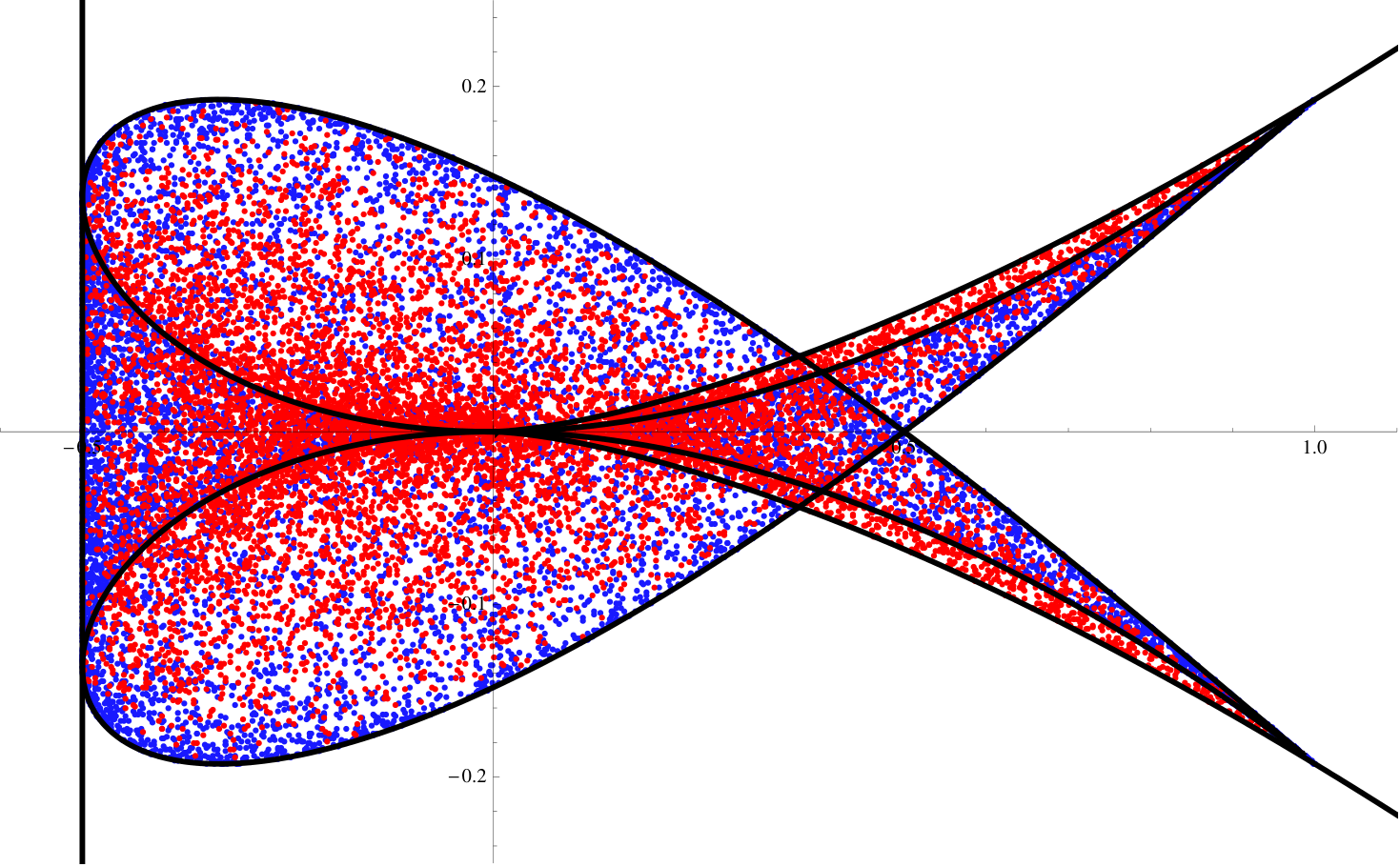
The flattened soccer ball is the compact region in that is depicted in Figure 2. In particular, is not convex. If the second coordinate were replaced by a homogeneous quadric then would be convex, by a theorem of Brickman [6].
We can quickly get an impression of the flattened ball by sampling points from the ball and plotting their images in . These are the red points in Figure 2. We next sample points from the sphere and we plot these in blue. Figure 2 shows the existence of two small regions with many red points but no blue points at all. This means that the image of the sphere is strictly contained in the image of the ball. In symbols, . The Zariski closure of the boundary of the image is given by the polynomials
Here, vanishes on the red boundary, while vanishes on the blue boundary.
For a triple of polynomials in , representing the pair , we define the algebraic boundary of to be the Zariski closure in of the topological boundary of . In addition to being compact, we also assume that is regular, i.e. the closure of the interior of contains . This excludes examples where lower-dimensional pieces stick out, like the Whitney umbrella. With these hypotheses, we can apply results in real algebraic geometry, found in (13, Lemma 3.1) and (19, Lemma 4.2), to conclude that the algebraic boundary is pure of dimension in . It is defined by the product of two squarefree polynomials and in . The curve is the branch locus of the map itself. It depends only on and but not on . The curve is the branch locus of the restriction of to the surface . It depends on . Note that is reducible in Example 1.
This paper is organized as follows. In Section 2 we study the algebraic geometry underlying our problem. If the data are generic polynomials then the curves and are irreducible. We determine their Newton polygons and singularities. In Section 3 we explore the global topology of the flattened soccer ball . We present upper and lower bounds on the number of connected components in its complement. Section 4 introduces tools from symbolic computation for deriving an exact representation of . Section 5 offers connections to convexity and to sum-of-squares techniques in polynomial optimization.
2 Algebraic Curves
A standard approach in algebraic geometry is to focus on the generic instance in a family of problems. This then leads to an upper bound for the algebraic complexity of the output that is valid for all special instances. In what follows we pursue that standard approach.
Suppose that and are generic inhomogeneous polynomials of degrees and in . The soccer ball and the map are defined as in (1) and (2). Let denote the squarefree polynomial that defines the branch locus of , and let be the squarefree polynomial that defines the branch locus of . These polynomials are unique up to scaling. They represent the algebraic boundary of . Both curves are in fact irreducible:
Theorem 2.1
For generic polynomials in , the boundary polynomials and of the flattened soccer ball are irreducible. Their Newton polygons are the triangles
The irreducible complex curves and are highly singular, with genera
The numbers of singular points of these curves in the complex affine plane are
In this statement, denotes the genus of the Riemann surface that is obtained by resolving the singularities of the curve . Equivalently, this is the geometric genus. The proof of Theorem 2.1 realizes the plane curves and as generic projections of smooth curves in -space. This implies that all their singular points are nodes (cf. [12]), and these are counted by the difference between the arithmetic genus and the geometric genus.
Table 1 underscores how singular our curves are. For instance, the last row concerns a general map of degree . The branch locus of that map restricted to the boundary surface has degree . A general plane curve of that same degree has genus . However, the genus of our curve is only , so it has singular points.
From the polygon in Theorem 2.1 we see that the curve has degree , and similarly for . When the input polynomials of degrees are not generic but special, these numbers serve as an upper bound. We take the sum of these numbers to get
Corollary 1
For any , the algebraic boundary of has degree at most
This bound is tight when the polynomials are generic relative to their degrees.
Remark 1
If and is arbitrary then the branch curve of the map has genus . This means the curve admits a parametrization by rational functions.
The two cases given in the third and fourth row of Table 1 will be of most interest to us. For each of them, we may assume that is the unit ball (3), but is arbitrary.
Example 2
If we flatten the unit ball (3) via a quadratic map () then the branch locus of is the rational sextic curve , with singular points. The branch curve of the restriction of to is the curve of degree and genus , so it has singular points. These two curves make up the boundary of .
If both and are homogeneous quadrics then the image of under is convex. This follows from (6, Theorem 2.1). More precisely, is a spectrahedral shadow, bounded by a curve of degree six. This scenario corresponds to the case in Table 1 of [20]. The image is generally not convex when one of the quadrics is not homogeneous. For instance, the image of the unit ball under the map is not convex.
Example 3
Proof (Proof of Theorem 2.1)
We consider two curves in affine -space . The curve is defined by the -minors of the Jacobian matrix of with respect to . This -matrix has general entries of degree in the first row and general entries of degree in the second row. By the Thom-Porteous-Giambelli Formula, we have . This expression equals . The curve is the complete intersection defined by the polynomial , which has degree , and the Jacobian determinant of with respect to , which has degree . By Bézout’s Theorem, . The hypothesis that and are generic ensure that and are smooth and irreducible. Their degrees are the quantities and in the statement.
Both of the results from algebraic geometry that were used in the previous paragraph (Thom-Porteous-Giambelli and Bézout) require certain genericity hypotheses on the geometric data to which they apply. These hypotheses are satisfied in our case because the given polynomials , and are assumed to have generic coefficients. See e.g. (17, Section 3.5.4).
The curves defined by and are the images of and under the map from to . Our first claim states that, for , the Newton polygon of the plane curve is the triangle , where .
We prove this using tropical geometry [15]. By genericity of and , the tropical curve in is the -dimensional fan with rays spanned by , , and , where each ray has multiplicity . Our goal is to compute the tropical curve in . This contains the image of under the tropicalization of the map . This is the piecewise-linear map that takes in to . Its image is the weighted ray in spanned by . The other rays of the tropical curve arise from the points of at which and vanish. We derive these using the method of Geometric Tropicalization, specifically (15, Theorem 6.5.11). The relevant very affine curve is , and the normal crossing boundary in the SNC pair is the divisor defined by on .
The surface meets the curve in points, and the divisorial valuations at these points map to the weighted ray in . Likewise, the surface meets in points, and their divisorial valuations create the weighted ray in . Hence the tropical plane curve consists of the three weighted rays specified by , and . This implies our assertion about the Newton polygons of and .
To prove the second assertion, about the genera of the two curves in question, we use the following two facts about general curves in . These are easily derived by computing the Hilbert series and then reading off the Hilbert polynomial. Recall that, for a curve with the Hilbert polynomial , the degree is and the arithmetic genus is . Moreover, if the curve is smooth, then its geometric genus equals the arithmetic genus.
- •
A smooth space curve defined by the -minors of a -matrix with rows of degrees and has degree and genus .
- •
The complete intersection of two general surfaces of degrees and in is a smooth curve of degree and genus .
The genus of the plane curve is equal to the genus of the space curve that maps to it, and similarly for and . So, it suffices to compute the genera of the affine curves and in . We may work with their projective closures and in . The curve has the determinantal representation as in the first bullet, with and . Substitution yields the desired formula for . The curve is the complete intersection of two surfaces in , of degree and . Substituting these expressions into , we obtain the desired formula for .
We can regard and as curves in the weighted projective plane given by the known Newton polygons. The genus of a general curve of the same degree is the number of interior lattice points on the Newton triangle. That number is equal to
Here is or as before. The number of singular points is the number above minus the genus of the curve. This gives the count in the last assertion of Theorem 2.1.
We used the computer algebra system Macaulay2 [10] to verify some of the entries in Table 1. Here is the Macaulay2 code we used for a typical computation with :
S = QQ[x,y,u,v,w];  h = u^2+v^2+w^2-1;
f = u*v-u*w+7*v^2+v*w+5*w^2+u+v+w+1;
g = u^2-u*v+u*w-v^2+v*w-w^2+u-v+w-1;
C1 = minors(2,jacobian(ideal(f,g)));
C2 = minors(3,jacobian(ideal(f,g,h)))+ideal(h);
p = first first entries gens
                 eliminate({u,v,w},C1+ideal(x-f,y-g))
Ip = radical(ideal(diff(x,p),diff(y,p),p));
{degree p, # terms  p, degree Ip}
q = first first entries gens
                 eliminate({u,v,w},C2+ideal(x-f,y-g))
Iq = radical(ideal(diff(x,q),diff(y,q),q));
{degree q, # terms  q, degree Iq}
The polynomials p and q have degrees and respectively. The command # terms verifies that all monomials in the Newton polygons appear with non-zero coefficients. The singular loci of the two curves are given by their radical ideals, Ip and Iq. Applying the command degree to these ideals verifies that the number of singular points is and respectively.
3 Topological Complexity
When a soccer ball gets flattened, one generally expects the planar image to be simply connected. However, it is quite possible for to have holes. In other words, the complement can have two or more connected components. In this section we present an explicit construction that makes this happen, with the number of holes being arbitrarily large.
The number of connected components of is at most the number of connected components of . The number of its holes is counted by the first Betti number of . The best upper bounds for Betti numbers of compact semialgebraic sets are due to Basu and Riener (1, Theorem 10) and Basu and Rizzie (2, Theorem 27). In our setting, the number of holes is bounded by if and by otherwise.
In what follows we assume that is the unit ball (3). The image is a compact connected subset of . We are interested in maps whose image is not simply connected. The construction we shall give furnishes the lower bound on the number of holes of . Based on Lissajous curves, it gives rise to some beautiful explicit examples.
The Chebyshev polynomials (of the first kind) are defined recursively by
Explicitly, the Chebyshev polynomials are
They satisfy the trigonometric identity . Fix relatively prime positive integers and with . Let denote the Lissajous curve
| (4) |
Its Zariski closure is the curve of degree with polynomial parametrization
For instance, Lissajous curve is the rational cubic . It is singular at .
Example 4
Figure 3 shows the Lissajous curve . This curve has singular points. This is the number of bounded regions in the complement of in .
Lemma 1
The curve has precisely complex singular points. All of these are real and are attained by two distinct values of in the trigonometric parametrization (4).
Proof
By the same argument as in the proof of Theorem 2.1, the Newton polygon of the Lissajous curve is contained in the triangle with vertices , and . The number of interior lattice points of that triangle is . This is the genus of the generic curve with that Newton polygon. And, it hence is an upper bound on the number of complex singular points of the special curve .
We next exhibit real singular points on that are in the image of (4). Pick any and any . Consider the angles
| (5) |
If , then and ; otherwise and . This means that and map to the same point, and the Lissajous curve has a node at that point. There are choices of pairs . Since the trigonometric parametrization (4) is -to- on the interval , this creates nodal singularities on . This argument is a modification of (4, Section 2.1). The lower bound we derived matches the upper bound in the previous paragraph, and this completes the proof.
We now apply this to flattening the soccer ball. Consider the map with
| (6) |
where is the degree- Chebyshev polynomial, and is a small constant. The map takes the soccer ball and creates a two-dimensional image with many holes in .
Example 5
Let and . The set is the region shown in Figure 4. It has precisely one hole. This picture was created by the following code in Mathematica, which produces a huge expression:
h = 1 - (u^2 + v^2 + w^2);
f = 2*u^2 - 1 + 1/10*v;  g = 4*u^3 - 3*u + 1/10*w;
S = Exists[{u, v, w}, h >= 0 && x == f && y == g];
SR = Resolve[S, Reals]
RegionPlot[SR, {x, -1.2, 1.2}, {y, -1.2, 1.2}, PlotPoints -> 50]
The command “Resolve” performs quantifier elimination.
The following is our main result in this section.
Theorem 3.1
Let be relatively prime and as above with sufficiently small. Then, the complement of in has connected components. The algebraic boundary of is an irreducible curve of degree at most . It is the branch locus of , so it is defined by the polynomial that was denoted by in Theorem 2.1.
Proof
The part of the curve that lies in the square is compact. We regard this as an embedded planar graph, where the vertices are the nodal singularities given in (5) together with the two degree endpoints, and the edges are the pieces of the Lissajous curve that connect the nodes and endpoints. This planar graph is -valent, the numbers of vertices, edges and faces satisfy and . This implies , i.e. the Lissajous curve has the correct number of holes.
As increases from to being positive, the curve gets replaced by a two-dimensional region. But the number of holes in the complement does not change.
The algebraic boundary of is given by the polynomials and that describe the branch curves of and respectively. However, in the present case, the curve does not exist because the Jacobian of the map has rank for all . The Jacobian determinant of with respect to is the irreducible polynomial
| (7) |
This is a polynomial of degree in which and occur linearly. The intersection of this surface with the unit sphere is an irreducible curve of degree at most . To compute the image of the curve, we substitute and into and into (7). This results in two polynomials in . Our task is to eliminate . We do this by taking the determinant of the Sylvester matrix with respect to . The non-constant entries in the Sylvester matrix have degree one or two in or . By examining their pattern in the matrix, we find that the determinant is a polynomial of degree at most .
Remark 2
We found experimentally that the Newton polygon of is the triangle with vertices , and , but we could not prove this.
Example 6
We return to the flattened soccer ball seen in the introduction. To draw this picture from scratch in Mathematica, we run the code in Example 5, modified as follows:
f = u*v + v*w + u*w; g = u*v*w;
For this input, the output of the quantifier elimination command Resolve equals:
(-(1/2) <= x <= 0 && y == 0) ||
   (y == -(1/(3*Sqrt[3])) && x == -(1/3)) ||
   (-(1/(3*Sqrt[3])) < y < 0 &&
      Root[2*#1^3 + #1^2 - y^2 & , 1] <= x <=
        Root[2*#1^3 + #1^2 - y^2 & , 2]) ||
   (y == 0 && Inequality[-(1/2), LessEqual, x, Less,
        0]) || (0 < y < 1/(3*Sqrt[3]) &&
      Root[2*#1^3 + #1^2 - y^2 & , 1] <= x <=
        Root[2*#1^3 + #1^2 - y^2 & , 2]) ||
   (y == 1/(3*Sqrt[3]) && x == -(1/3)) ||
   (x == -(1/2) && -(1/(3*Sqrt[6])) <= y <=
        1/(3*Sqrt[6])) || (-(1/2) < x < -(1/3) &&
      Root[729*#1^4 + #1^2*(-(92*x^3) + 6*x^2 + 48*x -
                   16) + 4*x^6 - 4*x^5 + x^4 & , 1] <= y <=
        Root[729*#1^4 + #1^2*(-(92*x^3) + 6*x^2 + 48*x -
                   16) + 4*x^6 - 4*x^5 + x^4 & , 4]) ||
   (x == -(1/3) && -(1/(3*Sqrt[3])) <= y <=
        1/(3*Sqrt[3])) ||
   (-(1/3) < x < (1/38)*(5*Sqrt[5] - 7) &&
      Root[729*#1^4 + #1^2*(-(92*x^3) + 6*x^2 + 48*x -
                   16) + 4*x^6 - 4*x^5 + x^4 & , 1] <= y <=
        Root[729*#1^4 + #1^2*(-(92*x^3) + 6*x^2 + 48*x -
                   16) + 4*x^6 - 4*x^5 + x^4 & , 4]) ||
   (x == (1/38)*(5*Sqrt[5] - 7) && -Sqrt[2*x^3 + x^2] <=
        y <= Sqrt[2*x^3 + x^2]) ||
   ((1/38)*(5*Sqrt[5] - 7) < x < 16/43 &&
      Root[729*#1^4 + #1^2*(-(92*x^3) + 6*x^2 + 48*x -
                   16) + 4*x^6 - 4*x^5 + x^4 & , 1] <= y <=
        Root[729*#1^4 + #1^2*(-(92*x^3) + 6*x^2 + 48*x -
                   16) + 4*x^6 - 4*x^5 + x^4 & , 4]) ||
   (16/43 <= x <= 1/2 && -(Sqrt[x^3]/(3*Sqrt[3])) <=
        y <= Sqrt[x^3]/(3*Sqrt[3])) ||
   (1/2 < x < 1 && (-(Sqrt[x^3]/(3*Sqrt[3])) <= y <=
           Root[729*#1^4 + #1^2*(-(92*x^3) + 6*x^2 + 48*x -
                      16) + 4*x^6 - 4*x^5 + x^4 & , 2] ||
         Root[729*#1^4 + #1^2*(-(92*x^3) + 6*x^2 + 48*x -
                      16) + 4*x^6 - 4*x^5 + x^4 & , 3] <= y <=
           Sqrt[x^3]/(3*Sqrt[3]))) ||
   (x == 1 && (y == -(1/(3*Sqrt[3])) ||
         y == 1/(3*Sqrt[3])))
This is a quantifier-free formula for the flattened soccer ball in Figure 2. Most readers will find such an output hard to understand. The next section offers an alternative.
4 Exact Representation of the Image
Quantifier elimination for polynomial systems over is usually performed by cylindrical algebraic decomposition [8], abbreviated CAD. Many variants can be found in the recent literature, including truth table invariant CAD [5] and variant quantifier elimination [11]. CAD represents a semialgebraic set as a union of cells. In dimension one this would be a disjoint union of points and open intervals. Several implementations of CAD are now available, including QEPCAD [7], and the packages RegularChains [14] and ProjectionCAD [9] in Maple. In Example 6, we experimented with the implementation of CAD in Mathematica.
This section is purely expository, aimed at all mathematicians and their students. We show how to obtain a meaningful CAD “by hand” for all instances with parameters . Experts and CAD developers might find this useful as a family of test cases.
Consider the curve in defined by the polynomial . Our image is the closure of a union of connected components of its complement. We compute a partition of that refines the partition given by . A key step is to label each open piece in the finer partition. We then test which pieces lie in , and we report the labels of those that do.
Algorithm 1 describes what we do. The geometric idea is to project onto the -axis. The critical points of that projection come in four flavors: singular points of , singular points of , points in the intersection , and smooth points on with vertical tangent lines. The critical -values are the -coordinates of all real critical points.
Two consecutive critical -values define a vertical strip. Here, the behavior of the curve segments does not change as varies. In particular, curve segments do not cross or change direction. Curve segments pass from the left to the right over two consecutive critical -values, and they divide the vertical strip into open regions. Two of them are unbounded and hence irrelevant. Each bounded region is either contained in or is disjoint from .
Our description of has three parts: the polynomials and that define the algebraic boundary, the critical -values, and a set of pairs of positive integers. A pair determines a region in as follows. The -coordinates are between the -th and -st critical -value, and the -coordinates lie between -th and -st curve segment in the -direction.
Steps 1 and 2 of Algorithm 1 can be done with Macaulay2, as shown at the end of Section 2. Step 3 is more delicate because and are fairly large, even when are small. The task is to compute the critical -values of the polynomials and , and also the -coordinates of the common zeros of and . To find these -values symbolically, we compute three resultants of two polynomials in with respect to . Namely, we compute
| (8) |
At this stage one might compute the real roots of these three univariate polynomials in . This can be done numerically using various methods, including the numerical algebraic geometry package in Macaulay2. However, we did not do this in our computations. Instead, we identify the real roots of our three resultants purely symbolically, using the command Solve with the option Reals in Mathematica. Solve tries to write each solution explicitly in terms of radicals, and if unsuccessful, it creates a representation as a root of a polynomial.
Since is compact, we can enclose it inside an appropriate cube in . We sample points with rational coordinates from that cube, and we throw out points that do not satisfy . For instance, if is the unit sphere, then we first uniformly sample points from the cube and keep the points that satisfy .
Step 4 is probabilistic. As the number of samples grows to infinity, every region in the CAD of will be reached and certified eventually. For any finite number of samples, there is a positive probability that some region is missed. Our approach can be turned this into a deterministic method by selecting a sample point in each region and deciding whether it has a preimage in . This amounts to testing whether a semialgebraic set in is non-empty. The best known algorithm for deciding non-emptiness of a semialgebraic set is by Renegar [18]. In practice this can be done using implementations of CAD, but we decided not to pursue the deterministic variant in the present study.
In our examples we are also interested in deciding which regions of lie in . Note the distinction between the colors in Figure 2. For instance, to obtain points on the boundary of the unit ball, we uniformly sample points from the square , keep the points that satisfy , and create two boundary points with .
In Step 5, we use binary search to determine such that is between the -th and -st element of the list . The symbolic representation derived in Mathematica is suitable for doing this. To be precise, we did the binary search with the following commands:
Block[{$ContextPath}, Needs["Combinatorica‘"]]
k = Combinatorica‘BinarySearch[C, x]-1/2
The real roots of can again be computed using Mathematica command Solve. We now illustrate Algorithm 1 by applying it to the instance that launched this project.
Example 7
Fix as in Example 1. The first part of the output are the polynomials and at the end of Example 1. The second part is the list of critical -values:
| (9) |
The third part is a list which represents a partition of into regions:
The output above represents a quantifier-free formula for the flattened soccer ball. Using symbolic computation, we can assign one of the labels to any sample point . For instance, consists of the six regions .
From our output, we drew the picture in Figure 5. For this, we used the coordinates of all singular points and branch points of . Branching occurs along the vertical tangent line . The real singular points are , , , , , , , , , , . Four pairs of critical points have the same -coordinates, seen in (9). The singular points and the vertical tangent line are the black landmarks in Figure 5. The regions are shown in different colors. The six regions in are colored light.
The output of Algorithm 1 can be interpreted as a semialgebraic formula for , as follows: Consider as a univariate polynomial in . Write down its Sturm sequence. Let denote the number of sign changes in that sequence evaluated at . The formula for the region is a disjunction over all the possible sign assignments of the Sturm sequence with sign changes, in conjunction with being between the -th and -st critical -value. Such a formula will again be hard to read, just like the Mathematica output displayed at the end of Section 4. A description like Example 7, accompanied by a picture like Figure 5, seems to be the most human-friendly way to represent the result of flattening a soccer ball.
We next discuss a more serious example, where the Resolve command does not terminate. It will demonstrate the pros and cons of the exact symbolic approach.
Example 8
Fix as before, so is the unit ball. We select and randomly from polynomials of degree and respectively. This means we are now in the regime covered by Theorem 2.1. Note the fourth line in Table 1 marked . The following instance, picked for us by Macaulay2, corresponds to the picture in Figure 6:
The polynomial that describes the branch locus of has degree and terms. The polynomial that describes the branch locus of has degree and terms. In both cases, these numbers count exactly the lattice points of the Newton triangles in Theorem 2.1.
For Step 3 we compute three univariate polynomials in , namely the resultants in (8). The resultant of and has degree with real roots. The resultant of and has degree with real roots. The resultant of and has degree with real roots. All real roots are different, so the total number of critical -values is . In Step 4 we sample points from the cube and from its boundary, and we record their images under . In Step 5, we run over these points in , and we identify the labels of the regions that contain these points. Some regions are very small. It takes a long time to identify them. We found that is the union of the following regions:
Out of the bounded segments between the critical -values, precisely arise from . The left-most segments and the right-most segments do not arise. In the list above, the first pair refers to -coordinates between critical -values labeled #12 and #13, which are approximately and . The corresponding -coordinates are between the -nd and -rd root of , regarded as a polynomial in , with fixed in segment #12.
Figure 7 shows that the situation is delicate. The regions can be very small, even for curves of degree . For example, consider the critical -values labeled #33 and #34. They are and . The unique critical point over #33 is an intersection point of and . The unique critical point over #34 is a node of . They are shown in Figure 7.
In Figure 7(a) we scaled the -axis so that it shows the vertical strip #33. The -axis is left unscaled, so that we can see all curve segments in that strip. It looks like the blue curve has two segments and the red curve has four segments. However, two more blue segments are eclipsed by the relevant red segment. The truth becomes visible in Figure 7(b), where we also scale the -axis. The critical point on the right is a node of the blue curve and it does not lie on the red curve . The left critical point lies in . Our careful analysis also shows that , although this is not visible in Figure 6. Between critical -values labeled #15 and #19, the lower boundary is given by the red curve .
5 Convexity and Optimization
The problem of computing images of maps is of considerable interest in polynomial optimization. Magron, Henrion and Lasserre [16] developed a method for this based on outer approximations. Our study is complementary to theirs, in the sense that we do not consider approximations but we seek exact descriptions. A related question is how to compute and represent the convex hull of the image . This issue will be addressed later in this section.
We start our discussion with a few examples where both and are convex. In what follows we retain the assumption that , so is the unit ball in . This can be folded into a convex polygon in various interesting ways.
Example 9
It is easy to find quadratic polynomials and such that maps the soccer ball onto a triangle or a rectangle. Figure 1 shows a map onto a square. Here are two explicit maps that work. If and then is the square with vertices , and is the triangle with vertices . The boundary polynomials are and . For a second example let be defined by and . Now the flattened soccer ball is the triangle with vertices , while is the triangle with vertices . The difference is not a convex set.
If we pass from quadratic maps to cubic maps then we can create other polygons.
Example 10
Use the cubic Chebyshev polynomial to define via
The image is the regular hexagon with vertices at and .
This raises the question whether we can prescribe to be any polyhedral shape. Ueno [21] proves that every unbounded convex polygon in is the image of under a polynomial map. It is not known, if his construction extends to polynomial images of the unit ball.
Problem 1
Let be an arbitrary convex polygon in . Construct explicit polynomials and in such that .
Our next topic is the flattenings of pancakes. These arise as special scenarios when we flatten soccer balls. Indeed, suppose that the map depends only on two of the variables, say
Then the image of is the same as the image under of the unit disk . In symbols, . The unit disk serves the role of our pancake.
Example 11
Magron et al. (16, Example 1) illustrate their method for the map
It is instructive to compare their output with that of Algorithm 1. The exact description of the flattened pancake begins with the two polynomials that define the algebraic boundary:
The projection of the curve onto the -axis has four critical points:
Our quantifier-free description of the planar region consists of the five pairs:
Figure 8 shows where these five regions are colored in yellow, orange, green, blue and purple. The critical points are black, and the boundary curve is red.
Outer approximations of the kind studied in [16] tend to work best when one is interested not in the image itself but in its convex hull . Its extreme points are the solutions for the parametrized family of optimization problems
| (10) |
The function is called the support function of the set . From the values of this function one obtains a description of the convex hull of as an intersection of closed halfspaces:
The optimization problem in (10) can be equivalently written as
Both the objective function and the constraint are given by polynomial functions. Although in general this can be difficult to solve, good upper bounds can be obtained using sum of squares methods [3]. This method minimizes subject to
where and are sums of squares. The solution satisfies the inequality . Furthermore, restricting the polynomials to have fixed degree, this is a semidefinite optimization problem, so it can be solved efficiently. Since , we obtain an outer approximation of the convex hull:
| (11) |
The right hand side is a spectrahedral shadow, so it is a desirable set in the context of [3]. If one is lucky then equality holds in (11) and a semidefinite representation of has been obtained. From our earlier algebraic perspective, such a representation still involves quantifiers. Any quantifier-free formula has to account for supporting lines that were created when passing from to its convex hull. Those lines are bitangents of our curve .
Acknowledgements.
Pablo Parrilo was supported by AFOSR FA9550-11-1-0305. Bernd Sturmfels was supported by NSF grant DMS-1419018 and the Einstein Foundation Berlin. Part of this work was done while the authors visited the Simons Institute for the Theory of Computing at UC Berkeley.References
- (1) S. Basu and C. Riener: Bounding the equivariant Betti numbers of symmetric semi-algebraic sets, Advances in Mathematics 305 (2017), 803–855.
- (2) S. Basu and A. Rizzie: Multi-degree bounds on the Betti numbers of real varieties and semi-algebraic sets and applications, arXiv:1507.03958.
- (3) G. Blekherman, P.A. Parrilo and R. Thomas: Semidefinite optimization and convex algebraic geometry, MOS-SIAM Series on Optimization 13, SIAM, 2013.
- (4) M. Bogle, J. Hearst, V. Jones and L. Stoilov: Lissajous knots, J. Knot Theory Ramifications 3 (1994), 121–140.
- (5) R. Bradford, J. Davenport, M. England, S. McCallum and D. Wilson: Truth table invariant cylindrical algebraic decomposition, J. Symbolic Comput. 76 (2016), 1–35.
- (6) L. Brickman: On the field of values of a matrix, Proceedings of the American Mathematical Society 12 (1961), 61–66.
- (7) C.W. Brown: QEPCAD B: A program for computing with semi-algebraic sets using CADs, SIGSAM Bull. 37 (2003), 97–108.
- (8) G.E. Collins: Quantifier elimination for real closed fields by cylindrical algebraic decompostion, Springer Lecture Notes in Computer Science 33 (1975), 134–183.
- (9) M. England, D. Wilson, R. Bradford and J.H. Davenport: Using the Regular Chains Library to build cylindrical algebraic decompositions by projecting and lifting, in Mathematical Software – ICMS 2014, Springer, 2014.
- (10) D. Grayson and M. Stillman: Macaulay2, a software system for research in algebraic geometry, available at www.math.uiuc.edu/Macaulay2/.
- (11) H. Hong and M. Safey El Din: Variant quantifier elimination, J. Symbolic Comput. 47 (2012), 883–901.
- (12) T. Johnsen: Plane projections of a smooth space curve, in Parameter Spaces, 89–110, Banach Center Publications 36, Polish Academy of Sciences, 1996.
- (13) T. Kahle, K. Kubjas, M. Kummer and Z. Rosen: The geometry of rank-one tensor completion, SIAM J. Appl. Algebra Geometry (2017).
- (14) F. Lemaire, M. Moreno Maza and Y. Xie: The RegularChains library in MAPLE, SIGSAM Bull. 39 (2005), 96–97.
- (15) D. Maclagan and B. Sturmfels: Introduction to Tropical Geometry, Graduate Studies in Mathematics 161, American Mathematical Society, 2015.
- (16) V. Magron, D. Henrion and J.-B. Lasserre: Semidefinite approximations of projections and polynomial images of semialgebraic sets, SIAM J. Optim. 25 (2015), 2143–2164.
- (17) L. Manivel: Symmetric Functions, Schubert Polynomials, and Degeneracy Loci, SMF/AMS Texts and Monographs 6, Cours Spécialisés 3, American Mathematical Society, Société Mathématique de France, 2001.
- (18) J. Renegar: On the computational complexity and geometry of the first-order theory of the reals, J. Symb. Comput. 13 (1992), 255–352.
- (19) R. Sinn: Algebraic boundaries of SO(2)-orbitopes, Discrete Comput. Geometry 50 (2013), 219–235.
- (20) R. Sinn and B. Sturmfels: Generic spectrahedral shadows, SIAM J. Optim. 25 (2015), 1209–1220.
- (21) C. Ueno: On convex polygons and their complements as images of regular and polynomial maps of , J. Pure Appl. Algebra 216 (2012), 2436–2448.