Measuring the trilinear neutral Higgs boson couplings in the minimal supersymmetric standard model at $e^{+}e^{-}$ colliders in the light of the discovery of a Higgs boson

The ATLAS [1] and CMS [2] experiments at the CERN Large Hadron Collider have independently observed a resonance at about 125-126 GeV. The ATLAS experiment after collecting data at an integrated luminosity of 4.8 fb^-1 at $\sqrt{s}$ = 7 TeV, and 5.8 fb^-1 at $\sqrt{s}$ = 8 TeV confirmed the evidence for the production of a neutral boson with a measured mass of 126.0 $\pm$ 0.4(stat) $\pm$ 0.4(syst) GeV, with a significance of 5.9 $\sigma$. The CMS experiment after collecting 5.1 fb^-1 at 7 TeV, and 5.3 fb^-1 at 8 TeV reported an evidence of a neutral boson at 125.3 $\pm$ 0.4(stat) $\pm$ 0.5(syst) GeV, with a significance of 5.8 $\sigma$. The CMS and ATLAS collaborations have now combined their analysis, which leads to the mass of the reported resonance as [3]

The properties of the discovered state are consistent with the properties of the standard model (SM) Higgs boson. Nevertheless, this discovery opens up the possibility of searches for new physics beyond the standard model. Since the Higgs sector suffers from the problems of naturalness and hierarchy, a light Higgs boson is technically unnatural in standard model. Supersymmetry (SUSY) [4] is at present the leading candidate for physics beyond the SM in which a light Higgs boson, as discovered at the CERN LHC, is technically natural. The simplest implementation [5, 6] of the idea of supersymmetry at weak scale is the minimal supersymmetric standard model (MSSM). In MSSM the Higgs sector is more complex than the SM Higgs sector, and consists of two Higgs doublet superfields ($H_{1}$ and $H_{2}$). After gauge symmetry breaking the physical Higgs sector consists of two $CP$-even Higgs bosons ($h^{0},H^{0};m_{h^{0}}<m_{H^{0}}$), one $CP$-odd Higgs boson ($A^{0}$), and two charged states ($H^{\pm}$). Although gauge invariance and supersymmetry fix the quartic couplings of the Higgs bosons in the MSSM in terms of the $SU(2)_{L}$ and $U(1)_{Y}$ gauge couplings, $g$ and $g^{\prime}$, respectively, there remain two independent parameters that describe the Higgs sector of the MSSM. These are conveniently chosen to be the mass of the $CP$-odd Higgs boson ($m_{A^{0}}$), and the ratio of the vacuum expectation values of the neutral components of the two Higgs fields, $\tan\beta\equiv<H_{2}^{0}>/<H_{1}^{0}>$. All the Higgs boson masses and the Higgs couplings in the MSSM can, then, be described, at the tree level, in terms of these two parameters. Discovery of more than one Higgs boson will, thus, be an indication of an extension of the SM, SUSY being the most favored candidate. It is, therefore, important to try to discover an extended Higgs sector, if it exists, at the LHC. On the other hand it is also crucial to discover the supersymmetric partners of the SM particles, including the squarks, gluinos and sleptons, as well as the neutralinos and charginos.

In the absence of any signal for supersymmetric partners of the SM particles, it is appropriate to ask the question whether nonobservation of an extended Higgs sector would imply that the new physics is at a much higher energy scale. This question is related to the decay patterns [8, 9, 7] of the Higgs bosons of MSSM. This in turn is dependent on the Higgs couplings in the MSSM, and their deviation from the corresponding SM Higgs couplings. Apart from the couplings of Higgs bosons to the SM particles, which can be different from those of the corresponding SM Higgs couplings, the trilinear Higgs couplings can be very different in MSSM as compared to the SM trilinear Higgs coupling.

The measurement of the trilinear Higgs couplings [10, 11, 12, 13, 14, 15] is an important step in the reconstruction of the Higgs potential, and thereby confirm the Higgs mechanism as the origin of the spontaneous breaking of the gauge symmetries in the SM (and in MSSM). As explained above, the tree level Higgs sector of the MSSM is described by only two parameters ($m_{A^{0}}$ and $\tan\beta$). At the tree level the trilinear Higgs self couplings of the MSSM can also be described in terms of the same two parameters. In this paper we consider the question of measurement of the trilinear Higgs couplings in the MSSM at a high energy electron-positron collider in the light of the observation of the Higgs boson at the CERN LHC, which we identify with the lightest Higgs boson of the MSSM.

The plan of this paper is as follows. In Section II we recall the basic features of the Higgs sector of the minimal supersymmetric standard model and discuss the implications of the 125 GeV Higgs identification for the mass of the heavier Higgs boson ($H^{0}$) of the model, especially its dependence on the parameter space of the MSSM. In Section III we summarize the tree level as well as radiatively corrected trilinear Higgs couplings in the MSSM and discuss their dependence on the different parameters. In Section IV, we estimate the cross-section for different heavy Higgs production processes and discuss its branching ratios to light Higgs pair in the MSSM parameter space. In Section V we highlight the regions in the ($m_{A^{0}},\tan\beta$) plane where some of the MSSM Higgs trilinear couplings can be measured. In Section VI we summarize our results and conclusions.

To begin with, and to have a proper perspective, we recall that the potential for the physical Higgs boson in the SM can be written as

The nondecoupling scenario has also been explored recently in context of LHC 8 TeV data [28]. But as far as measurement of MSSM Higgs bosons trilinear coupling is concerned, the decoupling scenario is a more viable scenario. Therefore, in the following we shall consider only the MSSM with decoupling scenario while discussing the trilinear Higgs couplings. The nondecoupling scenario is discussed in some detail in [8].

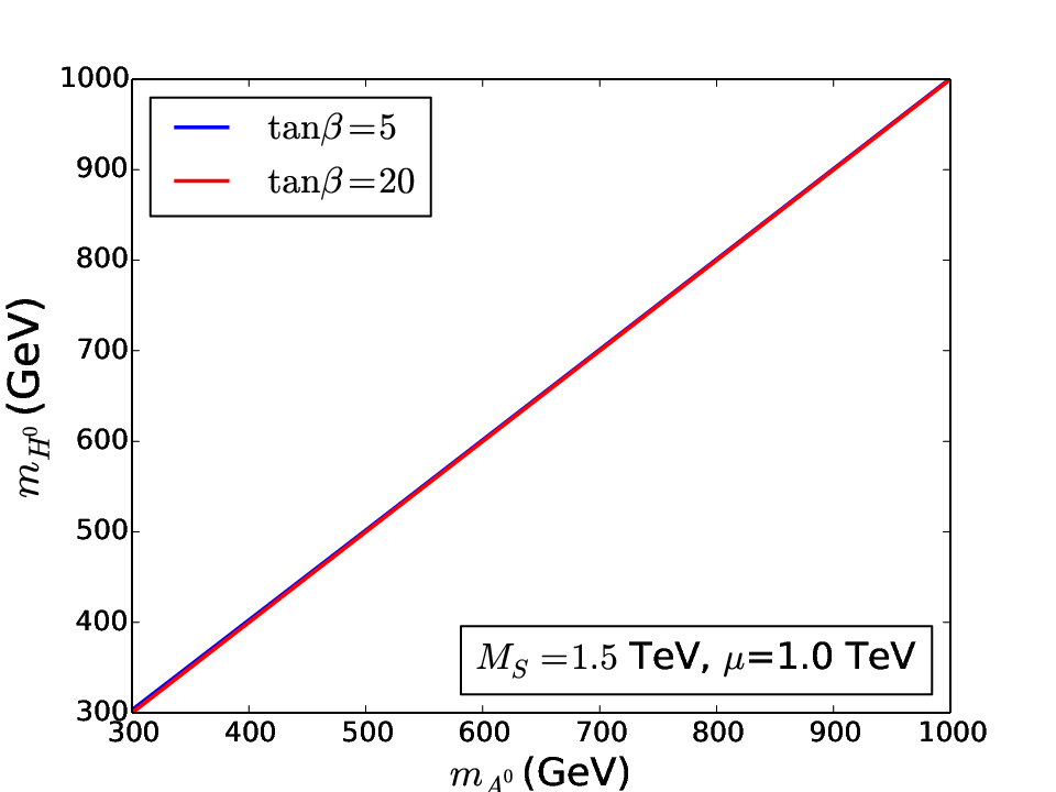
In order to identify the state observed at the CERN LHC with the lightest Higgs boson of the MSSM, we shall adjust the supersymmetry breaking soft trilinear parameter $A_{t}$ so as to get $m_{h^{0}}$ in the range 122-128 GeV, corresponding to a 3 GeV theoretical uncertainty in the Higgs mass calculations. Having fixed $m_{h^{0}}$, we have performed a numerical scan of the MSSM parameter space using CalcHEP [29] which uses SuSpect [30] for MSSM spectrum calculations. SuSpect checks the stability of potential and calculates the spectrum only for stable points. For our analysis we use set of input parameters which are consistent with known experimental constraints, and also which have the possibility of leading to the supersymmetry spectra that may be observable in the upcoming experiments. We do this in order to have low energy supersymmetry as a viable option for solving the naturalness and hierarchy problem of the standard model. Using this procedure, we have calculated the dependence of the heavy $CP$-even Higgs boson mass $m_{H^{0}}$ on $\mu$ for different values of $\tan\beta,$ and the SUSY breaking scale $M_{S}$, which is defined to be $\sqrt{m_{\tilde{t_{1}}}m_{\tilde{t_{2}}}}$, where $m_{\tilde{t_{1}}}$ and $m_{\tilde{t_{2}}}$ are the masses of the two stop states. This dependence is shown in Fig.1. This Fig. shows that $m_{H^{0}}$ does not depend significantly on $\mu$. For a given value of $\tan\beta$ it depends weakly on $M_{S}$. However, $m_{H^{0}}$ has a significant dependence on $m_{A^{0}}$ and $\tan\beta$, and can be described in terms of these two parameters to a good accuracy when we use the fact that $m_{h^{0}}$ lies in the range 122-128 GeV. As an example, for one set of $M_{S}$, $\tan\beta$ and $m_{A^{0}}$ we show the values of the parameter $A_{t}$ with different values of $\mu$ in Table 1. For the considered range of $\mu$, $A_{t}$ does not change much. For $M_{S}$=1.5 TeV, typical range of $A_{t}$ is 2500-4000 GeV depending on $\tan\beta$.

We now discuss the question of the measurement of trilinear couplings of the neutral Higgs bosons ($h^{0},H^{0}$) of the minimal supersymmetric standard model. These couplings receive contributions at the tree level as well as from radiative corrections. We shall assume CP conservation throughout in this paper. Then the trilinear couplings can be written as[31]

where $\lambda^{0}$’s are the tree level values of the couplings, and $\Delta\lambda$’s are the radiative corrections. In this paper we shall consider the one-loop approximation for the radiative corrections to the trilinear Higgs couplings. The leading two loop SUSY-QCD corrections to the trilinear couplings are available in the literature [32] which reduces the scale dependence of one-loop corrections but the contribution is very small as compared to the one-loop corrections. The tree-level couplings in units of $(\sqrt{2}G_{F})^{1/2}m_{Z}^{2}$ can be written as

We note that the Higgs sector depends on five parameters in the MSSM, $m_{A^{0}}$ and $\tan\beta$ from tree level mass matrix, and three parameters $A_{t}$, $\mu$ and $M_{S}$ from radiative corrections. Of these $M_{S}$ is fixed from nonobservation of colored particles to be greater than 1.5 TeV, and $A_{t}$ is used to fix the value of lightest Higgs mass ($m_{h^{0}}$). For fixed value of $\tan\beta$ we are left with two parameters $m_{A^{0}}$ and $\mu$. In Fig. 2 we show the variation of radiatively corrected trilinear couplings with respect to $m_{A^{0}}$ (for fixed value of $\mu$), and with respect to $\mu$ (for fixed value of $m_{A^{0}}$), respectively. In Fig. 2 (c) we show the trilinear couplings as a functions of $\tan\beta$ (for fixed value of $\mu$ and $m_{A^{0}}$). Most of the variation in the trilinear Higgs couplings comes from the variation of the radiative corrections, a fact which is shown in Fig. 3, where we plot only the radiative corrections to different trilinear Higgs couplings.

From these Figures, we can see that the trilinear couplings are sensitive to $m_{A^{0}}$ upto 500 GeV except the ones involving CP-odd Higgs boson. In Fig. 2 (c), we have shown the variation of trilinear Higgs couplings as a function of $\tan\beta$ for a value of $m_{A^{0}}$ = 300 GeV, with other parameters kept fixed, and this plot shows that trilinear couplings are weakly dependent on $\tan\beta$. In this paper we shall consider only the trilinear couplings $\lambda_{hhh}$ and $\lambda_{Hhh}$ between the neutral Higgs bosons $h^{0}$ and $H^{0}$.

We now consider the different processes at an $e^{+}e^{-}$ collider which can be used for the measurements of the trilinear Higgs couplings $\lambda_{hhh}$ and $\lambda_{Hhh}$ in the MSSM. These processes involve production of multiple Higgs bosons, to which we now turn.

Multiple light Higgs bosons ($h^{0}$) can be produced through heavy CP-even Higgs boson decays. For CP-even heavy Higgs boson production we consider Higgs-strahlung $e^{+}e^{-}\rightarrow ZH$, associated production with CP-odd Higgs boson $e^{+}e^{-}\rightarrow AH$, and $WW$ fusion mechanism $e^{+}e^{-}\rightarrow\nu_{e}\bar{\nu}_{e}H$. Feynman diagrams for these processes are shown in Figs. 4 and 5. Heavy Higgs boson $H^{0}$ subsequently decays to a pair of light Higgs bosons. The branching ratio of $H\rightarrow hh$ depends on trilinear Higgs coupling $\lambda_{Hhh}$,

Notice that this decay is kinematically forbidden in the non decoupling regime. The cross-sections for the Higgs-strahlung and associated production with CP-odd Higgs boson can be written as [33, 34, 11, 12, 13]

where $\lambda_{i}$ is the phase-space function, which corresponds to $\lambda(m_{i}^{2},m_{H^{0}}^{2};s)$, and is given by

and $v_{e}=4\sin^{2}\theta_{W}-1$, $a_{e}=-1$ are the Z boson-electron couplings.

On the other hand resonant $WW$ fusion cross-section for the light Higgs pair production can be written as [11, 12, 13]

where

with

The multiple Higgs production through non resonant $WW$ $\rightarrow$ $hh$ proceeds via the diagrams shown in the Fig. 5. The non-resonant fusion $WW\rightarrow hh$ cross-section in the effective $WW$ approximation can be written as

where

and $\hat{\sigma}_{WW}(x)$ can be written as [11, 12, 13]

where

and the exact forms of $g_{i}$ (i=0,..5) functions can be found in [11, 12, 13]. We note that there can be sizable deviations of the effective $WW$ approximation from the exact result. However, we shall use this approximation as an estimate in this paper.

and decay width for $A\rightarrow hZ$ is given by

We note that the Feynman diagrams shown in Fig. 7 will lead to $hhh$ final state through $A\rightarrow hZ$ decay, whereas we are interested in final states having $hh$ final state.

In Fig. 8 we show the cross-section for $e^{+}e^{-}$ $\rightarrow$ $HZ$, $HA$, $H\nu\bar{\nu}$, (Fig.4), $Ah$ (Fig. 6(d)) as a function of $m_{H^{0}}$ for different values of $\sqrt{s}$ and $\tan\beta$. The heavy Higgs production with CP-odd Higgs is the dominant production channel for $m_{H^{0}}$ $\leq$ 250 GeV. We can see that ($\sigma(e^{+}e^{-}\rightarrow Ah)$)/2 is of order of $\sigma(e^{+}e^{-}\rightarrow ZH)$ and $\sigma(e^{+}e^{-}\rightarrow H\nu\bar{\nu})$.

In Figs. 9 and 10, we show the branching fractions of heavy Higgs and pseudoscalar to different channels respectively for $\tan\beta$ = 5, 10. In this paper we have also considered supersymmetric particles in the final states, consistent with current experimental constraints. All the SUSY particles have masses $\approx$ $M_{S}$ except neutralinos and charginos. The neutralinos and charginos mass spectrum depends on the supersymmetry breaking gaugino mass parameters $M_{1}$ and $M_{2}$ as well as $\mu$ and $\tan\beta$. We recall that the chargino mass lower bounds from the LEP experiment imply [35]

We shall confine ourselves to the scenario where supersymmetry breaking gaugino masses $M_{i}$ ($i$ = 1, 2, 3) are equal at the grand unified scale. In this case the renormalization group evolution of $M_{i}$ implies $M_{1}$ $\approx$ 0.5 $M_{2}$ at the weak scale. We shall consider the parameter space consistent with these constraints.

We have plotted the $H$ and $A$ branching fractions for two benchmark values of $\mu$, $M_{1}$ and $M_{2}$. The neutralino and chargino mass spectrum for the benchmark points is given in Table 2. The second benchmark point has comparatively heavy spectrum. We observe that for $m_{A^{0}}$ $\approx$ $m_{H^{0}}$ $\geq$ 500 GeV, neutralino and chargino are the dominant decay modes of both $H$ and $A$, for a light neutralino and chargino spectrum. If these are heavy then $t\bar{t}$ is the dominant decay channel for low values of $\tan\beta$. In case of $H$ decay, below $t\bar{t}$ threshold both $b\bar{b}$ and $hh$ have appreciable branching fractions. For large $\tan\beta$ and heavy neutralino and chargino spectrum, $b\bar{b}$ is the dominant decay mode of the heavy Higgs boson as shown in Fig. 9 (d). Our aim is to study BR($H$ $\rightarrow$ $hh$) and BR($A$ $\rightarrow$ $hZ$), since the former involves the Higgs trilinear coupling and latter is background for multiple Higgs production processes. We can see from Fig. 10 that $A\rightarrow hZ$ branching fraction is negligible for values of $\tan\beta$ = 5 and 10. Below $\chi^{+}\chi^{-}$ threshold, $A$ $\rightarrow$ $b\bar{b}$ is the dominant decay channel for large value of $\tan\beta$.

The contours of constant values of BR($H$ $\rightarrow$ $hh$ ) are shown in Fig. 11 for the benchmark points. The BR($H$ $\rightarrow$ $hh$) decreases with increasing $\tan\beta$. Since the neutralino and chargino spectrum is heavy for the second benchmark point, BR($H\rightarrow\chi^{0}\chi^{0},\chi^{+}\chi^{-}$) is suppressed as compared to first benchmark point and consequently BR($H\rightarrow hh$) is enhanced. In all the plots we have varied the relevant parameters in a manner so that the lightest Higgs mass is in the range 122-128 GeV. The main parameter adjusted in this context is $A_{t}$. As already mentioned we have allowed a 3 GeV theoretical uncertainty in the Higgs mass calculations. If one wants to restrict to the range of 124-126 GeV for the mass of the Higgs boson, then we will have a corresponding slightly narrow band of $A_{t}$ values. In other words that will also reduce the range of values of the parameter $A_{t}$. But that minor variation in the $A_{t}$ values will not change our analysis significantly since $A_{t}$ parameter enters through one loop radiative corrections in the trilinear coupling calculations. Processes shown in Fig. 4 involve only trilinear coupling $\lambda_{Hhh}$, but Fig. 5 (c) and 6 (c) involve both $\lambda_{hhh}$ and $\lambda_{Hhh}$. Therefore one has to study non-resonant multiple Higgs production cross-section to measure $\lambda_{hhh}$ coupling.

In this Section we will compute the regions of ($m_{A^{0}}$,$\tan\beta$) plane where trilinear couplings $\lambda_{Hhh}$ and $\lambda_{hhh}$ can be measured. We calculate the heavy Higgs production cross-section using Eqs. 15, 16 and 18. The contours of $\sigma(H)\times BR(H\rightarrow hh)$ for $\sqrt{s}$ = 500 GeV and $\sqrt{s}$ = 1.5 TeV, respectively are shown in Fig. 12. In upper left and right panel, the outermost contours correspond to $\sigma(H)\times BR(H\rightarrow hh)$ $\approx$ 0.005 fb and .04 fb, respectively. The $\sigma(H)\times BR(H\rightarrow hh)$ decreases as we move diagonally upward in the $(m_{A^{0}}$,$\tan\beta)$ plane because $BR(H\rightarrow hh)$ decreases in this direction. As shown in Fig. 8, the heavy Higgs production cross-section increases for $\sqrt{s}$ = 1.5 TeV, therefore one can measure $\lambda_{Hhh}$ coupling with a lower luminosity.

The BR($H\rightarrow hh$) is directly proportional to $\lambda_{Hhh}$ and this branching ratio decreases with increasing $\tan\beta$ for fixed value of $m_{A^{0}}$. As discussed earlier, heavy Higgs production cross-section decreases with $m_{A^{0}}$. The $H$ branching ratio to $hh$ pair is kinematically forbidden for $m_{A^{0}}$ $\approx$ $m_{H^{0}}$ $\leq$ 250 GeV. Therefore, the lower left corner of $(m_{A^{0}}$,$\tan\beta)$ plane is the suitable region to measure $\lambda_{Hhh}$ coupling. We can see from the Fig. 12 that $\sigma(H)\times BR(H\rightarrow hh)$ is sensitive to the $\mu$ parameter. In other words, precise knowledge of neutralino and chargino spectrum is crucial in order to determine the $\lambda_{Hhh}$ coupling. For $\sqrt{s}$ = 1.5 TeV and heavy neutralino and chargino spectrum with $\tan\beta$ $\approx$ 10, $\sigma(H)\times BR(H\rightarrow hh)$ $\approx$ 0.4 fb. This cross-section is 0.05 fb for $\sqrt{s}$=500 GeV so with a luminosity of 500 fb ^-1, 25 events could be seen. This indicates only order of magnitude that can be reached but the actual number of events seen will be lowered by the efficiencies. The simulations of signal and background will depend on the detector sensitivity which is not the focus of this paper.

The $hh\nu_{e}\bar{\nu}_{e}$ final state produced through non-resonant $WW$ fusion involves both $\lambda_{hhh}$ and $\lambda_{Hhh}$ coupling. Having an estimate of the coupling $\lambda_{Hhh}$ from resonant $WW$ production process, we can use non-resonant $WW$ fusion process to measure the trilinear $\lambda_{hhh}$ coupling. In Fig. 13 we show the constant contours of the cross-section for the non-resonant $WW$ fusion process $\sigma(hh\nu_{e}\bar{\nu}_{e})$ in the $(m_{A^{0}},\tan\beta)$ plane. We can see that the cross-section $\sigma(hh\nu_{e}\bar{\nu}_{e})$ is almost independent of the values of $m_{A^{0}}$ and $\tan\beta$. The chances of the measurement of $\lambda_{hhh}$ are same in most of the $(m_{A^{0}},\tan\beta)$ parameter space. There is a small increase in the cross-section at the boundary $m_{H^{0}}^{2}$ $\approx$ 4 $m_{h^{0}}^{2}$ where Fig. 5(c) starts contributing through resonant process. Even with the 1000 fb ^-1 of luminosity at $\sqrt{s}$ = 500 GeV one could see only few events.

In Fig. 8 we have plotted the cross-section for the background process $e^{+}e^{-}\rightarrow Ah$ and BR ($A\rightarrow hZ$) in Fig. 10. Since BR ($A\rightarrow hZ$) is negligible this process will be suppressed for the considered parameter space. Also this kind of background events can be easily distinguished from the signal events by just looking at the $hh$ pair invariant mass distribution which will resonate in case of signal process.

We have carried out a detailed analysis of the measurement of trilinear couplings of the neutral CP-even Higgs boson, $\lambda_{Hhh}$ and $\lambda_{hhh}$, at an electron-positron collider. For this purpose we have identified the state observed at CERN Large Hadron Collider at $\approx$ 125 GeV with the lightest Higgs boson of the MSSM. This identification has been used to study the dependence of the mass of the heavier CP-even Higgs boson of the MSSM ($H^{0}$) on the parameter space of the MSSM, so as to get a handle on the mass of $H^{0}$. Furthermore, we have also used the lower bound on the chargino mass from the LEP experiments to constrain the parameter space of the MSSM. All these constraints have been used in our study of the trilinear couplings.

Our main purpose is to investigate various processes involving multiple Higgs bosons in the final state in $e^{+}$-$e^{-}$ collisions, consistent with the constraints summarized above. The production of the heavier Higgs bosons in $e^{+}e^{-}$ collisions can lead to multiple lighter Higgs bosons ($h^{0}$) in the final state, which can be used in the measurement of the trilinear couplings of the CP-even Higgs bosons.

We indicate the regions of the $(m_{A^{0}},\tan\beta)$ plane where trilinear coupling $\lambda_{Hhh}$ and $\lambda_{hhh}$ can be measured at the linear collider. The resonant heavy Higgs production processes are used to extract $\lambda_{Hhh}$ coupling. For $\sqrt{s}$= 1.5 TeV, $\tan\beta$ $\approx$ 8, the $\sigma(H)\times BR(H\rightarrow hh)$ $\approx$ 1 fb, and regions of $\tan\beta$ upto 10 and $m_{A^{0}}$ upto 450 can be explored for $\lambda_{Hhh}$ coupling measurement. However high luminosity is required to probe larger $\tan\beta$ values. For the measurement of the $\lambda_{hhh}$ coupling, we use light Higgs pair production through non-resonant WW fusion, and this cross-section is not very sensitive to $m_{A^{0}}$ and $\tan\beta$. Besides values of $m_{A^{0}}$ and $\tan\beta$, the information of neutralino and chargino masses is crucial for determining the trilinear couplings.

The work of P. N. Pandita is supported by the Department of Atomic Energy, India through its Raja Ramanna Fellowship. He would like to thank the Inter University Centre for Astronomy and Astrophysics, Pune for hospitality where part of this work was done. C. K. Khosa would like to thank Jayita Lahiri for many fruitful discussions.

In this Appendix we summarize the one-loop radiative corrections to the trilinear Higgs couplings in the MSSM [11, 12, 13, 31]. The radiative corrections, in units of $(\sqrt{2}G_{F})^{1/2}{m_{Z}^{2}}$ can be written as

References

- [1] G. Aad et al. [ATLAS Collaboration], Phys. Lett. B 716, 1 (2012) [arXiv:1207.7214 [hep-ex]].
- [2] S. Chatrchyan et al. [CMS Collaboration], Phys. Lett. B 716, 30 (2012) [arXiv:1207.7235 [hep-ex]].
- [3] G. Aad et al. [ATLAS and CMS Collaborations], Phys. Rev. Lett. 114, 191803 (2015) [arXiv:1503.07589 [hep-ex]].
- [4] J. Wess and J. Bagger, “Supersymmetry and supergravity,” Princeton, USA: Univ. Pr. (1992) 259 p.
- [5] H. P. Nilles, Phys. Rept. 110, 1 (1984).
- [6] P. Nath, R. L. Arnowitt and A. H. Chamseddine, “Applied N=1 Supergravity,” Lectures given at Conference (Trieste Particle Phys.1983:1), NUB-2613.
- [7] B. Ananthanarayan, J. Lahiri, P. N. Pandita and M. Patra, Phys. Rev. D 87, no. 11, 115021 (2013) [arXiv:1306.1291 [hep-ph]].
- [8] P. N. Pandita and M. Patra, Phys. Rev. D 89, 115010 (2014) [arXiv:1405.7163 [hep-ph]].
- [9] B. Ananthanarayan, J. Lahiri and P. N. Pandita, Phys. Rev. D 91, 115025 (2015) [arXiv:1507.01747 [hep-ph]].
- [10] A. Djouadi, H. E. Haber and P. M. Zerwas, Phys. Lett. B 375, 203 (1996) [hep-ph/9602234].
- [11] P. Osland and P. N. Pandita, Phys. Rev. D 59, 055013 (1999) [hep-ph/9806351].
- [12] P. Osland and P. N. Pandita, hep-ph/9911295.
- [13] P. Osland and P. N. Pandita, hep-ph/9902270.
- [14] A. Djouadi, W. Kilian, M. Muhlleitner and P. M. Zerwas, Eur. Phys. J. C 10, 27 (1999) [hep-ph/9903229].
- [15] L. Wu, J. M. Yang, C. P. Yuan and M. Zhang, Phys. Lett. B 747, 378 (2015), [arXiv:1504.06932 [hep-ph]].
- [16] J. R. Ellis, G. Ridolfi and F. Zwirner, Phys. Lett. B 262, 477 (1991).
- [17] Y. Okada, M. Yamaguchi and T. Yanagida, Prog. Theor. Phys. 85, 1 (1991).
- [18] H. E. Haber and R. Hempfling, Phys. Rev. Lett. 66, 1815 (1991).
- [19] M. Carena, J. R. Espinosa, M. Quiros and C. E. M. Wagner, Phys. Lett. B 355 (1995) 209.
- [20] H. E. Haber, R. Hempfling and A. H. Hoang, Z. Phys. C 75, 539 (1997).
- [21] M. Carena, H. E. Haber, S. Heinemeyer, W. Hollik, C. E. M. Wagner and G. Weiglein, Nucl. Phys. B 580, 29 (2000).
- [22] T. Li, Phys. Lett. B 728, 77 (2014) [arXiv:1309.6713 [hep-ph]].
- [23] P. N. Pandita, Phys. Lett. B 151, 51 (1985).
- [24] E. Boos, A. Djouadi, M. Muhlleitner and A. Vologdin, Phys. Rev. D 66, 055004 (2002) [hep-ph/0205160].
- [25] E. Boos, A. Djouadi and A. Nikitenko, Phys. Lett. B 578, 384 (2004) [hep-ph/0307079].
- [26] N. D. Christensen, T. Han and S. Su, Phys. Rev. D 85, 115018 (2012) [arXiv:1203.3207 [hep-ph]].
- [27] H. E. Haber, hep-ph/9510412.
- [28] B. Bhattacherjee, M. Chakraborti, A. Chakraborty, U. Chattopadhyay and D. K. Ghosh, Phys. Rev. D 93, 075004 (2016). [arXiv:1511.08461 [hep-ph]].
- [29] A. Belyaev, N. D. Christensen and A. Pukhov, Comput. Phys. Commun. 184, 1729 (2013) [arXiv:1207.6082 [hep-ph]].
- [30] A. Djouadi, J. L. Kneur and G. Moultaka, Comput. Phys. Commun. 176, 426 (2007) [hep-ph/0211331].
- [31] V. D. Barger, M. S. Berger, A. L. Stange and R. J. N. Phillips, Phys. Rev. D 45, 4128 (1992).
- [32] M. Brucherseifer, R. Gavin and M. Spira, Phys. Rev. D 90, 117701 (2014) [arXiv:1309.3140 [hep-ph]].
- [33] G. Pocsik and G. Zsigmond, Z. Phys. C 10, 367 (1981).
- [34] J. F. Gunion et al., Phys. Rev. D 38, 3444 (1988).
- [35] S. Schael et al. [ALEPH and DELPHI and L3 and OPAL and SLD and LEP Electroweak Working Group and SLD Electroweak Group and SLD Heavy Flavour Group Collaborations], Phys. Rept. 427, 257 (2006), [hep-ex/0509008].