Asynchronous Multi-Agent Primal-Dual Optimization
Abstract
We present a framework for asynchronously solving convex optimization problems over networks of agents which are augmented by the presence of a centralized cloud computer. This framework uses a Tikhonov-regularized primal-dual approach in which the agents update the system’s primal variables and the cloud updates its dual variables. To minimize coordination requirements placed upon the system, the times of communications and computations among the agents are allowed to be arbitrary, provided they satisfy mild conditions. Communications from the agents to the cloud are likewise carried out without any coordination in their timing. However, we require that the cloud keep the dual variable’s value synchronized across the agents, and a counterexample is provided that demonstrates that this level of synchrony is indeed necessary for convergence. Convergence rate estimates are provided in both the primal and dual spaces, and simulation results are presented that demonstrate the operation and convergence of the proposed algorithm.
I Introduction
Networked coordination and optimization have been applied across a broad range of application domains, such as sensor networks [1, 2, 3, 4], robotics [5], smart power grids [6, 7], and communications [8, 9, 10]. A common feature of some applications is the (sometimes implicit) assumption that communications and computations occur in a synchronous fashion. More precisely, though no agent may have access to all information in a network, the information it does have access to is assumed to be up-to-date and/or computations onboard the agents are assumed to occur concurrently.
One can envision several reasons why these synchrony assumptions may fail. Communications may interfere with each other, slowing data transmissions, or else they may occur serially over a shared channel, resulting in delays when many messages must be sent. In other cases it may simply be undesirable to stay in constant communication in a network due to the energy required to do so, e.g., within a team of battery-powered robots. Apart from communication delays, it may be the case that some agents produce new data, such as a new state value, faster than other agents, leading to mismatches in update rates and thus mismatches in when information becomes available. Regardless of their cause, the resulting delays are often unpredictable in duration, and the timeliness of any piece of information in a network with such delays typically cannot be guaranteed. While one could simply have agents pause their computations while synchronizing information across a network, it has been shown that asynchronous algorithms can outperform their synchronous counterparts which pause to synchronize information [11, Section 6.3.5][12, Section 3.3]. Accordingly, this paper focuses on asynchronous algorithms for multi-agent optimization.
In particular, this paper considers multi-agent convex optimization problems that need not be separable, and its structural novelty comes from the introduction of a centralized cloud computer and its associated communications model. The cloud’s role is to aggregate centralized information and perform centralized computations for the agents in the network, and the motivation for including a cloud computer comes from its ability to communicate with many devices and its ability to provide ample processing power remotely. However, the cloud’s operations take time to perform specifically because they are centralized, and although the cloud adds centralized information to a network, the price one has to pay for this centralized information is that it is generated slowly. As such, the proposed algorithmic model has to take this slowness into account.
In this paper we consider problems in which each agent has a local cost and local set constraint, and in which the network itself is associated with a non-separable coupling cost. The agents are moreover subject to non-separable ensemble-level inequality constraints11 1 The work here can include equality constraints without any further changes, though we focus only on inequality constraints for notational simplicity. that could, for example, correspond to shared resources. To solve these problems, we consider a primal-dual approach that allows the agents’ behavior to be totally asynchronous [11, Chapter 6] (cf. partially asynchronous [11, Chapter 7]), both when communicating among themselves and when transmitting to the cloud. However, we do require that the cloud’s transmissions to the agents always keep the dual variable’s value synchronized among the agents. This synchrony is verified to be necessary in Section VI, where a counterexample shows that allowing the agents to disagree upon the value of the system’s dual variable can preclude convergence altogether. The dual variable’s value is the lone point of synchrony in the presented algorithm, and all other aspects of the system are designed to strive toward operating as asynchronously as possible in a general optimization setting.
To produce such an algorithm, we apply a Tikhonov regularization to the Lagrangian associated with the problem of interest. This regularization causes the algorithm to only approximately solve optimization problems, and error bounds are provided in terms of the regularization parameters, along with a choice rule for selecting these parameters to enforce any desired error bound. The regularization we use induces a tradeoff between speed and accuracy in the optimization process, and it is shown that requiring a less accurate solution allows the algorithm to converge faster and vice versa.
We also make use of an existing framework for asynchronous optimization [11, Sections 6.1-6.2][13], which accommodates general unconstrained or set-constrained problems. This framework hinges upon the ability to construct a sequence of sets satisfying certain properties which admit a Lyapunov-like convergence result, and we show that our regularization guarantees the ability to construct this sequence of sets as long as the problem satisfies mild assumptions. We also provide novel convergence rate estimates in both the primal and dual spaces that explicitly account for the delays in the system. The contribution of this work thus consists of an asynchronous primal-dual optimization algorithm together with its convergence rates.
There exists a large corpus of work on multi-agent optimization that is related to the work here. In [11] a range of results are gathered on asynchronous multi-agent optimization (for problems without functional constraints or with linear equality constraints) in Chapters 6 and 7. Earlier work on asynchronous algorithms can be traced back to [14] and [15], which consider fixed points of certain classes of operators. Long-standing optimization algorithms known as the Jacobi and Gauss-Seidel methods are also covered in [11] for linear problems in Section 2.4. Linear consensus type problems are studied in [16], including cases in which identical time delays are associated with the communication channels. The framework in [11, Sections 6.1-6.2] is the most general, and we therefore use it as our starting point for optimization in the primal space.
A key difference between our work and earlier work is that we asynchronously solve general constrained convex optimization problems which, in general, need not satisfy the conditions in [11, 14, 15]. The work in [17] also solves constrained optimization problems asynchronously, though it requires bounded communication delays between agents and has each agent updating both a full primal vector and a full dual vector. In the current paper, communication delays do not have a uniform bound, and each agent updates only its own state as would be the case, e.g., in a team of robots.
Two other relevant and well-known algorithms of current interest are gossip algorithms and the alternating direction method of multipliers (ADMM). Here we do not consider gossip-type algorithms since they either require synchronous communications among the agents or, in the asynchronous case, allow only one communication channel to be active at a time [18], and our aim is to support communication models that are as general as possible by allowing any number of links to be active at a time.
In contrast to this, ADMM essentially imposes a Gauss-Seidel structure among the primal updates made by the agents [19]. Related work in [20] presents an asynchronous variant of ADMM, though it requires bounded delays and updates of all primal and dual variables onboard each agent, neither of which are required here. The algorithm we present can be viewed as a method related to ADMM that allows all agent behaviors to be essentially arbitrary in their timing. This provides a great degree of flexibility in the agents’ primal updates by not requiring any particular ensemble update rule or bounded delays, or requiring an agent to update all variables in the system.
The remainder of the paper is organized as follows. Section II describes the optimization problem to be solved and the regularization used. Then Section III gives a rule for choosing regularization parameters to limit errors in the system. Next, Section IV provides the asynchronous algorithm that is the main focus of the paper. Then Section V proves convergence of the asynchronous algorithm and provides convergence rates for it. We show in Section VI that synchrony in the dual variable is indeed a necessary condition for convergence. Section VII presents simulation results for the asynchronous algorithm, and Section VIII concludes the paper.
II Multi-Agent Optimization
This section gives a description of the problems under consideration and establishes key notation. To that end, the symbol without a subscript always denotes the Euclidean norm. We use the notation to denote the vector with its component removed, i.e.,
| (1) |
We also define the index set for all , and we will use the term “ensemble” to refer to aspects of the problem that involve all agents.
II-A Problem Statement
This paper solves convex optimization problems over networks comprised by agents. The agents are indexed over , and agent has an associated decision variable, , with , and we allow for when . Each agent has to satisfy a local set constraint, expressed by requiring , where we assume the following about each .
Assumption 1
For all , the set is non-empty, compact, and convex.
Note that Assumption 1 allows for box constraints, which are common in multi-agent optimization. We will also refer to the ensemble decision variable of the network, defined as where . Assumption 1 guarantees that is also non-empty, compact, and convex.
Agent seeks to minimize a local objective function which depends only upon . Together, the agents also seek to minimize a coupling cost which depends upon all states and can be non-separable. We impose the following assumption on and each .
Assumption 2
For all , the function is convex and (twice continuously differentiable) in . The function is convex and in .
Gathering these costs gives
| (2) |
and when Assumptions 1 and 2 hold, has a well-defined minimum value over .
We consider problems with ensemble-level inequality constraints, namely we require that the inequality
| (3) |
hold component-wise, under the following assumption.
Assumption 3
The function is convex and in .
In particular, does not need to be separable. At the ensemble level, we now have a convex optimization problem, stated below.
Problem 1
| minimize | (4) | |||
| subject to | (5) | |||
On top of the problem formulation itself, Section IV will specify an architecture that provides a mixture of distributed information sharing among agents and centralized information from a cloud computer. As a result, the solution to Problem 1 will involve a distributed primal-dual algorithm since such an algorithm is implementable in a natural way on the cloud-based architecture. Towards enabling this algorithm, we enforce Slater’s condition [21, Assumption 6.4.2] which enables us to find a compact set that contains the optimal dual point in Problem 1.
Assumption 4
(Slater’s condition) There exists a point such that .
II-B An Ensemble Variational Inequality Formulation
Under Assumptions 1-4 we define an ensemble variational inequality in terms of Problem 1’s Lagrangian. The Lagrangian associated with Problem 1 is defined as
| (6) |
where and denotes the non-negative orthant of . By definition, is convex for all and is concave for all . These properties and the differentiability assumptions placed upon and together imply that and are monotone operators on their respective domains. It is known that Assumptions 1-4 imply that a point is a solution to Problem 1 if and only if it is a saddle point of [22], i.e., it maximizes over and minimizes over so that it satisfies the inequalities
| (7) |
for all and . From Assumptions 1-4 it is guaranteed that a saddle point exists [23, Corollary 2.2.10].
Defining the symbol to denote a saddle point via and using to denote an arbitrary point in , we define the composite gradient operator
| (8) |
Then the saddle point condition in Equation (7) can be restated as the following ensemble variational inequality [23, Page 21].
Problem 2
Find a point such that for all .
II-C Tikhonov Regularization
Instead of solving Problem 2 as stated, we regularize the problem in order to make it more readily solved asynchronously and to enable us to analyze the convergence rate of the forthcoming asynchronous algorithm. The remainder of this paper will make extensive use of this regularization. First we define -strong convexity for a differentiable function.
Definition 1
A differentiable function is said to be -strongly convex if
| (9) |
for all and in the domain of .
We now regularize the Lagrangian using constants and to get
| (10) |
where we see that is -strongly convex and is -strongly concave (which is equivalent to being -strongly convex). Accordingly, and are strongly monotone operators over their domains. We also define and replace the subscripts and with the single subscript for brevity when we are not using specific values of and . We now have the regularized composite gradient operator,
| (11) |
The strong monotonicity of and together imply that itself is strongly monotone, and Assumptions 1-4 imply that has a unique saddle point, [23, Theorem 2.3.3]. We now focus on solving the following regularized ensemble variational inequality.
Problem 3
Find the point such that for all .
As a result of the regularization of to define , the solution will not equal . In particular, for a solution to Problem 2 and the solution to Problem 3, we will have and . Thus the regularization done with and affords us a greater ability to find saddle points asynchronously and, as will be shown, the ability to estimate convergence rates towards a solution, but does so at the expense of accuracy by changing the solution itself. While solving Problem 3 does not result in a solution to Problem 2, the continuity of over suggests that using small values of and should lead to small differences between and so that the level of error introduced by regularizing is acceptable in many settings. Along these lines, we provide a choice rule for and in Section III that enforces any desired error bound for certain errors due to regularization.
There is a well-established literature regarding projection-based methods for solving variational inequalities like that in Problem 3, e.g., [23, Chapter 12.1]. We seek to use projection methods because they naturally fit with the mixed centralized/decentralized architecture to be covered in Section IV, though it is required that be Lipschitz to make use of such methods. Currently, cannot be shown to be Lipschitz because its domain, , is unbounded. To rectify this situation, we now determine a non-empty, compact, convex set which contains , allowing us to solve Problem 3 over a compact domain. Below, we use the unconstrained minimum value of over , which is well-defined under Assumptions 1 and 2. We have the following result based upon [24, Chapter 10].
Lemma 1
Let be a Slater point of . Then
| (12) |
Proof: See [25], Section II-C.
If is not available, any lower bound on can be used in defining , and the above construction is still valid when using such a lower bound in conjunction with any Slater point . Having defined , we see that the norm of the gradient of can be uniformly upper-bounded for all , and is therefore Lipschitz. Denote its Lipschitz constant by . We now define a synchronous, ensemble-level primal-dual projection method for finding based on [24]. It relies on the Euclidean projections onto and , denoted and , respectively.
Algorithm 1
Let and be given. For values , execute
| (13) | ||||
Here and are stepsizes whose values will be determined in Theorems 1 and 2 in Section V. Algorithm 1 will serve as a basis for the asynchronous algorithm developed in Section IV, though, as we will see, significant modifications must be made to this update law to account for asynchronous behavior in the network.
III Bounds on Regularization Error
In this section we briefly cover bounds on two errors that result from the Tikhonov regularization of . For more discussion, we refer the reader to Section 3.2 in [26] for regularized Lagrangian methods and to Chapter 12.2 in [23] for a discussion of regularization error in variational inequalities.
For any fixed choice of and , denote the corresponding solution to Problem 3 by . It is known that as and across a sequence of problems, the solutions , where is the solution to Problem 2 with least Euclidean norm [23, Theorem 12.2.3]. Here, we are not interested in solving a sequence of problems for evolving values of and because of the computational burden of doing so; instead, we solve only a single problem. It is also known that an algorithm with an iterative regularization wherein and tend to zero as a function of the iteration number can also converge to [27], though here it would be difficult to synchronize changes in the regularization parameters across the network. As a result, we proceed with a fixed regularization and give error bounds in terms of the regularization parameters we use.
Our focus is on selecting the parameters and to satisfy desired bounds on errors introduced by the regularization. First we present error bounds and then we cover how to select and to bound these errors by any positive constant.
III-A Error Bounds
Below we use the following four constants:
| (14) |
We first state the error in optimal cost.
Lemma 2
Proof: See [26, Lemma 3.3].
Next we bound the constraint violation that is possible in solving Problem 3.
Lemma 3
Proof: See [26, Lemma 3.3].
III-B Selecting Regularization Parameters
We now discuss one possible choice rule for selecting and based upon Lemmas 2 and 3. Both lemmas suggest using to achieve smaller errors and, given that we expect , we choose . Suppose that there is some maximum error specified for Lemmas 2 and 3. The following result provides sufficient conditions for enforcing this bound by choosing and appropriately.
Proposition 1
Let be given. For
| (17) |
choosing regularization parameters and gives
| (18) |
IV Asynchronous Optimization
In this section, we examine what happens when primal and dual updates are computed asynchronously. The agents compute primal updates and the cloud computes dual updates and, because the cloud is centralized, the dual updates in the system are computed slower than the primal updates are. Due to the difference in primal and dual update rates, we will now index the dual variable, , over the time index and will continue to index the primal variable, , over the time index . In this section we make use of the optimization framework in Sections 6.1 and 6.2 of [11]. Throughout this section, discussions will have the same value of onboard all agents simultaneously, and this is shown to be a necessary condition for convergence in Section VI.
IV-A Per-Agent Primal Update Law
The exact update law used by agent will be detailed below. For the present discussion, we need only to understand a few basic facts about the distribution of communications and computations in the system. Agent will store values of some other agents’ states in its onboard computer, but will only update its own state within that state vector; states stored by agent corresponding to other agents will be updated only when those agents send their state values to agent . Because these operations occur asynchronously, there is no reason to expect that agents and (with ) will agree upon the values of any states in the network.
As a result, we index each agent’s state vector using a superscript: agent ’s copy of the state of the system is denoted and agent ’s copy of its own state is denoted . In this notation we say that agent updates but not for any . The state value is precisely the content of messages from agent to agent and its value onboard agent is changed only when agent receives messages from agent (and this change occurs immediately when messages are received by agent ).
To prevent unnecessary communications among the agents, we only require two agents to communicate if each needs the other’s state value in its computations. We make this notion precise in the following definition.
Definition 2
Agent is an essential neighbor of agent (where ) if depends upon . The set of indices of all essential neighbors of agent is called its essential neighborhood, denoted .
We illustrate the role of Definition 2 in defining communications among the agents in the following example.
Example 1
Consider a system with four agents with scalar states. For all , we have , and the constraints are and , with . For , we find that . As a result, agent ’s essential neighborhood is . We also find , and . As a result, agents and need only to communicate with each other and store each other’s states; neither needs to communicate with agents or at any point, nor to store the states of agents and . Similarly, agents and communicate and store each other’s states, but never communicate with agents and and therefore do not store their states. Agents that communicate states with each other do not need to do so simultaneously and can do so with any timing. Then at each timestep, there are four possible directed edges that can be active, and the union of all communication graphs over all timesteps is shown in Figure 1.
Here we see that the agents’ communications need not comprise a graph which is complete, nor even one which is connected in any sense. What results then is a system in which there may be multiple groups of agents which do not interact at all and which may indeed not even know of each other’s existence, though they are jointly solving an optimization problem.
Clearly if and only if , and thus agent both sends information to and receives information from its essential neighbors. While each agent only needs to store the states of its essential neighbors, we proceed as though each agent stores a full state vector in order to circumvent the need to track different dimensions of agents’ states. For agent , one can assume that is fixed at zero for all . Rather than considering a fixed communication topology and analyzing an optimization algorithm developed over that topology, Example 1 shows that we take the opposite approach: the information dependencies in the system determine which agents must communicate because these dependencies define the agents’ essential neighborhoods. Of course, in some cases, it will be difficult for two agents to communicate and they will do so only occasionally and without any specified schedule, and this is permitted by the asynchronous problem formulation we develop below.
The agents’ primal updates also do not occur concurrently with dual updates (which will be computed by the cloud). It is therefore necessary to track which dual variable the agents currently have onboard. At time , if agent has in its onboard computer, we denote agent ’s copy of by .
Each agent is allowed to compute its state updates using any clock it wishes, regardless of the timing of the other agents’ clocks. We use the symbol to denote a virtual global clock which contains the clock ticks of each agent’s clock, and can be understood as containing ordered indices of instants in time at which some number of agents compute state updates. Without loss of generality we take . We denote the set of time indices at which agent computes its state updates22 2 If computing a state update takes some non-zero number of timesteps, we can make the set of times at which agent ’s computation of a state update completes. For simplicity we assume that computing a state update takes agent zero time and that state updates are computed by agent at the points in time indexed by . by , i.e.,
| (21) |
At times agent does not compute any state updates and hence does not change at these times, though can still change if a transmission from another agent arrives at agent at time . We note that and the sets need not be known by the agents as they are merely tools used in the analysis of the forthcoming asynchronous algorithm. We also take as the set of ticks of the dual update clock in the cloud without loss of generality, though there need not be any relationship between and .
Suppose that agent computes a state update at time and then begins transmitting its state to agent also at time . Due to communication delays, this transmission may not arrive at agent until, say, time . Suppose further that agent ’s next transmission to agent does not arrive at agent until time . It will be useful in the following discussion to relate the time (at which the first transmission arrives) to the time (at which it was originally computed by agent ). Suppose at time , with onboard all agents, that agent has some value of agent ’s state, denoted . We use to denote the time at which the value of was originally computed by agent . Above, , and because the value of will not change again after until time , we have for all . We similarly define for all to fulfill the same role for transmissions of state values from agent to the cloud: at time in the cloud, is the time at which agent computed the state value it most recently sent to the cloud33 3 The agents can send multiple state values to the cloud between dual updates, though only the most recent transmission from agent to the cloud will be kept by the cloud.. For all , , and we have by definition, and we impose the following assumption on , , , and for all and .
Assumption 5
For all the set is infinite, and for a sequence in tending to infinity we have
| (22) |
for all . Furthermore, the set is infinite and for a sequence in tending to infinity we have
| (23) |
for all .
Requiring that be infinite guarantees that no agent will stop updating its state and Equation (22) guarantees that no agent will stop sending state updates to its essential neighbors. Similarly, being infinite guarantees that the cloud continues to update and Equation (23) ensures that no agent stops sending its state to the cloud. Assumption 5 can therefore be understood as ensuring that the system “keeps running.”
For a fixed , agent ’s update law is written as follows (where ):
| (24) | ||||
| (25) |
This update law has each agent performing gradient descent in its own state and waiting for other agents to update their states and send them to the others in the network. This captures in a precise way that agent immediately incorporates transmissions from other agents into its current state value and that such state values will generally be “out-dated,” as indicated by the presence of the term on the right-hand side of Equation (25).
IV-B Cloud Dual Update Law
While optimizing with onboard, the agents compute some number of state updates using Equation (24) and then send their states to the cloud. It is not assumed that the agents send their states to the cloud at the same time or that they do so after the same number of state updates. Once the cloud has received states from the agents, it computes and sends to the agents, and then this process repeats. Assumption 5 specified that these operations do not cease being executed, and we impose the following basic assumption on the sequence of updates that take place in the system.
Assumption 6
- a.
When the cloud sends to the agents, it arrives in finite time.
- b.
Any transmission originally sent from agent to agent while they have onboard is only used by agent if it is received before .
- c.
All transmissions arrive in the order in which they were sent.
- d.
There is an increasing sequence of times such that only is used in the agents’ state updates at timesteps satisfying .
Assumption 6.a is enforced simply to ensure that the optimization process does not stall and is easily satisfied in practice. Assumption 6.b is enforced because parameterizes
| (26) |
which is the point the agents approach while optimizing with onboard. Suppose that a message from agent is sent to agent while they have onboard but is received after they have onboard. We will in general have so that the arrival of agent ’s message to agent effectively redirects agent away from and toward , delaying (or preventing) progress of the optimization algorithm. With respect to implementation, little needs to be done to enforce this assumption. All communications between agents can be transmitted along with the timestamp of the dual variable onboard the agent sending the message at the time it was sent. The agent receiving this message can compare the value of in the message with the timestamp of the dual variable it currently has onboard, and any message with a mismatched timestamp can be discarded. Assumption 6.b can therefore be implemented in software without further constraining the agents’ behavior or the optimization problem itself.
Assumption 6.c will be satisfied by a number of communication protocols, including TCP [28, Section 13], which is used on much of the internet, and does not constrain the agents’ behavior because it can be enforced in software by choosing an applicable communication protocol. It is enforced here to prevent pathological behavior that can prevent the optimization from converging at all. Assumption 6.d enforces that the agents use the same value of the dual variable in their updates. Assumption 6.d is the lone point of synchrony in the system and is necessary for convergence of the asynchronous algorithm. This necessity is verified by a counter-example in Section VI wherein violating only Assumption 6.d causes the system not to converge.
After the agents have taken some number of steps using and have sent their states to the cloud, the cloud aggregates these states into a vector which we denote , defined as
| (27) |
Then we adapt the dual update in Algorithm 1 to account for the time the cloud spends waiting to receive transmissions from the agents, giving
| (28) |
IV-C Asynchronous Primal-Dual Update Law
We now state the full asynchronous primal-dual algorithm that will be the focus of the remainder of the paper. Below we use the notation to denote the set of times at which agent sends its state to the cloud. We also use the notation to denote the set of times at which agent sends its state to agent ; if , then . Note that need not have any relationship to or and that agent need not know as it is merely a tool used for analysis. Similarly, does not need to have any relationship to or and does not need to be known by any agent. We state the algorithm with the cloud waiting for each agent’s state before computing a dual update because this will typically be the desired behavior in a system. However, we do point out how to eliminate this assumption and the impact of this removal in Remark 4 in the next section.
Algorithm 2
Step 0: Initialize all agents and the cloud with and . Set and .
Step 1: For all and all ,
if , then agent sends to agent (though it may not be received for some time).
Step 2: For all and all , execute
| (29) | ||||
| (30) |
Step 3: If , agent sends to the cloud. Set . If all components of have been updated since the agents received , the cloud computes
| (31) |
and sends to the agents. Set .
Step 4: Return to Step 1.
V Convergence of Asynchronous Primal-Dual Method
In this section we examine the convergence properties of Algorithm 2 and develop its convergence rates. For clarity of presentation, we first show results that assume that all agents send their states to the cloud before the cloud computes each dual update. Once the main results of this section are established, we explain how to eliminate this Assumption in Remark 4.
V-A Block Maximum Norm Basics
First we consider the agents optimizing in the primal space with a fixed . We will examine convergence using a block-maximum norm similar to that defined in Section 3.1.2 of [11]. First, for a vector , we can decompose into its components as , and we refer to each such component of as a block of ; in Algorithm 2, agent updates block of . Using the notion of a block we have the following definition.
Definition 3
For a vector comprised of blocks, with the block being , the norm is defined as44 4 For concreteness we focus on the -norm, though the results we present can be extended to some more general weighted block-maximum norms of the form , where and for all . .
We have the following lemma regarding the matrix norm induced on by . In it, we use the notion of a block of a matrix. For , the block of is the matrix formed by rows with indices through in , and we denote the block of by .
Lemma 4
For all ,
| (32) |
Proof: For the block of , let be the entry of that block and let be the unit sphere in . Then for any and we have
| (33) |
Each term on the right-hand side of Equation (33) is manifestly positive so that summing over every block gives
| (34) |
which we can write in terms of as
| (35) |
Then, taking the maximum over all blocks, we have
| (36) |
for all , and the result follows by taking the supremum over .
We also have the following elementary lemma relating norms of vectors.
Lemma 5
For all ,
| (37) |
Proof: We find
| (38) |
and then take the square root.
V-B Convergence in the Primal Space
We now examine what happens when the agents are optimizing in between transmissions from the cloud. We consider the case of some fixed onboard all agents and as in Section IV we use . Under these conditions, the agents are asynchronously minimizing the function
| (39) |
until arrives from the cloud. To assess the convergence of Algorithm 2 in the primal space, we define a sequence of sets to make use of the framework in Sections 6.1 and 6.2 of [11]. These sets must satisfy the following assumption which is based on the assumptions in those sections.
Assumption 7
With a fixed value of and a fixed onboard all agents, the sets satisfy:
- a.
- b.
- c.
For all , there are sets satisfying
(40) - d.
For all and , , where .
Unless otherwise noted, when writing for some vector , the set is chosen with the largest value of that makes the statement true. Assumptions 7.a and 7.b require that we have a nested chain of sets to descend that ends with . Assumption 7.c allows the blocks of the primal variable to be updated independently by the agents while still guaranteeing that progress toward is being made. Assumption 7.d guarantees forward progress down the chain of sets whenever an agent computes a state update. More will be said about this assumption and its consequences below in Remark 1.
Recalling that is the (maximum, over ) Lipschitz constant of , we define the constant
| (41) |
We then have the following lemma that lets us determine the value of based upon .
Lemma 6
For and we have . Furthermore the minimum value of is
| (42) |
Proof: See Theorem 3 on page 25 of [29].
We proceed under the restrictions that and for the remainder of the paper. To simplify the presentation of results in this section, for all we assume that all agents simultaneously received at some time . This serves the same role as in Assumption 6.d, though the agents do not actually need to receive at the exact same time and indeed any means of enforcing Assumption 6.d will suffice. We retain this assumption on for the simplicity it provides below.
For each , we define the quantity
| (43) |
which is the “worst-performing” block onboard any agent with respect to distance from . For a fixed value of we define each element in the sequence of sets as
| (44) |
By definition, at time we have for all , and moving from to requires contracting toward (with respect to ) by a factor of . We have the following proposition.
Proof: By definition for all . From Equation (44), we see that
| (45) |
Because , we have , so that for we find
| (46) |
giving as well. Then for all and Assumption 7.a is satisfied.
We see that
| (47) | ||||
| (48) | ||||
| (49) |
which follows because is a norm. Then Assumption 7.b is satisfied as well.
For Assumption 7.c, the definition of lets us easily decompose . In particular, we see that
| (50) |
for all . Immediately then we have
| (51) |
from which it is clear that and thus that Assumption 7.c is satisfied.
Finally, we show that Assumption 7.d is satisfied. For a fixed and fixed take some . Recall the following exact expansion of :
| (52) | ||||
| (53) | ||||
| (54) |
where we have defined as
| (55) |
Using the non-expansive property of with respect to on , we find that for
| (56) | ||||
| (57) | ||||
| (58) | ||||
| (59) | ||||
| (60) | ||||
| (61) | ||||
| (62) |
where the third equality follows from Equation (54) and where the last inequality follows from Lemma 4. For any choice of , the -strong monotonicity and -Lipschitz properties of give , which implies that the eigenvalues of are bounded above by and below by for all . Using this fact and that is symmetric, we see that
| (63) | ||||
| (64) | ||||
| (65) |
where and denote the minimum and maximum eigenvalues of a matrix, respectively. Then from Equation (62), and the fact that by hypothesis, we find
| (66) |
so that as desired.
We comment on one consequence of Assumption 7 in particular below where we use the notation
| (67) |
Remark 1
Suppose at time agent has state vector and . Then Assumption 7.d implies that . Suppose, before any other agent transmits an updated state to agent , that agent performs another update of its own state. Just before the second update, is equal to with the entry for replaced with the update just computed, ; all other entries of remain unchanged from . Because no other agents’ states have changed, we still have and, as a result, . In general, here precisely because has not changed. Due to the fact that , the second update performed by agent results in once more, though, in general, no further progress, e.g., to , can be made without further updates from the other agents. Then while an agent is waiting for updates from other agents, its progress toward can be halted, though it does not “regress” backwards from, say, to .
V-C Single-Cycle Primal Convergence Rate Estimate
The structure of the sets enables us to extract a convergence rate estimate in the primal space. To demonstrate this point, consider the starting point of the algorithm: all agents have onboard some state and dual vector . Suppose that agent takes a single gradient descent step, say at time , from with held fixed. From Assumption 7.d, this results in agent having . Once agent transmits the state to its essential neighbors, and once all other agents themselves have taken a descent step and transmitted their states to their essential neighbors, say, at time , agent will have . Agent ’s next descent step, say at time , then results in . Then the process of communicating and descending repeats. To keep track of how many times this process repeats, we have the following definition.
Definition 4
After the agents all have just received , the first cycle ends as soon as (i) each agent has computed a state update and (ii) each agent has sent that updated state to all of its essential neighbors and it has been received by them. Subsequent cycles are completed when the preceding cycle has ended and criteria (i) and (ii) are met again, with any number of cycles possible between and .
It is possible for one agent to compute and share several state updates with the other agents within one cycle if some other agent in the network is updating more slowly. For a fixed value of onboard all agents and a common initial state , the first cycle will move each agent’s copy of the ensemble state from to , the second cycle will move it from to , etc. When the agents have onboard, we use to denote the number of cycles the agents complete before the first agent sends its state to the cloud for use in computing . We see that with onboard, the agents complete cycles to reach the set and the cloud therefore uses an element of to compute . In particular, using Assumption 7.d and the construction of the sets , this means that the convergence rate is geometric in the number of cycles completed:
| (68) |
Crucially, it need not be the case that all agents have the same state at the beginning of each cycle for this rate estimate to apply. We show this in deriving a general primal convergence rate in the following lemma.
Lemma 7
Proof: Suppose the agents just received from the cloud. For all we have from the definition of . Then when agent computes a state update the result is . When the agents have completed one cycle after receiving , say by time , we have . Iterating this process, after cycles agent ’s copy of the ensemble state moves from to for all . Then, when the agents send their states to the cloud, agent sends an element of . Then we have and, by definition, .
One can impose further assumptions, e.g., that a cycle occurs every ticks of , in which case the exponent of in Equation (69) becomes , though for generality we do not do so.
V-D Overall Convergence Rates
Towards providing a convergence rate estimate in the dual space, we first present the following lemma.
Lemma 8
For any primal-dual pairs and such that
| (70) |
we have
| (71) |
In addition,
| (72) |
Proof: See [26, Lemma 4.1].
We now prove approximate convergence in the dual space and estimate the rate of convergence there.
Theorem 1
Let all hypotheses of Lemma 7 hold and let the dual step-size satisfy
| (73) |
where . Then for all
| (74) |
where , is the diameter of , and is the maximum diameter among the sets , .
Proof: Using the non-expansive property of the projection operator and expanding we find
| (75) | ||||
| (76) | ||||
Adding inside the last set of parentheses, expanding, and applying Lemma 8 then gives
| (78) |
Next, we have
| (79) |
where expanding and re-arranging gives
| (80) |
Substituting Equation (80) into Equation (78) then gives
| (81) |
Taking , we find that
| (86) |
Substituting Equation (86) into Equation (84), and using the Lipschitz property of , we find
| (87) |
| (88) |
Using this in Equation (87) gives
| (89) |
where the result follows by summing over .
Remark 2
Theorem 1 shows that convergence in the dual space is governed by three terms. The first term decays as and represents a contraction toward . The next two terms are essentially error terms that result from not equaling ; to see this, note that an exact dual method would have , causing the sum in Theorem 1 to vanish, leaving only the contracting term. We see that larger values of lead closer to , causing the algorithm to approximate an ordinary dual algorithm, thus leading to smaller errors.
In addition, the term outside the sum indicates that past errors contribute less to the overall dual error, with old error terms accumulating powers of over time. To make faster progress using the asynchronous algorithm, one can have the agents perform small numbers of cycles for small values of and then increase as becomes large. Such a strategy makes later error terms small while weighting earlier error terms only minimally, giving a small overall error.
We now present a result on primal convergence in Algorithm 2.
Theorem 2
Let the primal step-size and let all hypotheses of Lemma 7 hold. Then for the sequence of primal vectors aggregated by the cloud, , we have
| (90) |
Convergence in the primal space is then governed by two terms, one of which behaves like a contraction whose exponent is and the other which is a constant multiple of the dual error, and we again find that completing more cycles improves accuracy. We also have the following tradeoff between speed and accuracy induced by the regularization of .
Remark 3
Theorem 2, Proposition 1 and Lemmas 6 and 7 together reveal a fundamental tradeoff between convergence rate and accuracy in the primal space. On the one hand, Proposition 1 shows that smaller values of lead to smaller errors while larger values of lead to larger errors. On the other hand, Lemma 6 shows that larger values of lead to smaller values of , and both Lemma 7 and Theorem 2 show that smaller values of lead to faster convergence through the primal space, while smaller values of cause to approach the value , thereby slowing convergence. Then smaller values of lead to smaller errors at the expense of slower convergence, while larger values of cause the system to converge more quickly, but to a point that is further away from .
A similar tradeoff applies to as well: Lemmas 2 and 3 show that smaller values of can lead to smaller errors, though the definition of in Theorem 1 shows that a larger value of decreases , leading to faster convergence. The appropriate balance of convergence speed and accuracy of a solution depends upon the problem being solved, though, taken together, these results give one the tools to quantitatively balance these two objectives.
One can also see the use of regularizing in Theorems 1 and 2. If one were to set , then we would find and primal updates would not make any progress toward in Lemma 7. Such a case would also cause the construction of the sets to break down as no “descent” down this sequence of sets could be shown. Similarly, if one were to set , we would find , in which case the only way to avoid moving away from in the dual space would be to set , thereby forestalling all progress in the dual space. Through their roles in determining and (and the use of these constants in the convergence analysis presented), it is evident that regularizing with and is essential to the analysis presented here.
We now point out how to formulate convergence rate estimates without having each agent send a state update to the cloud before it computes each dual update.
Remark 4
If one allows the cloud to compute dual updates before receiving a state update from each agent, then Lemma 7 should be modified to account for only some values of changing from . In particular, if agents send state updates to the cloud before it computes and do not, we find
| (93) |
Propagating this through Theorems 1 and 2 gives overall primal and dual convergence rate estimates for this case as well. In doing so, one finds that executing a cloud update without a state update from each agent can significantly harm convergence and it will usually be preferred to have the cloud wait until it has received state information from all agents before each dual update.
VI Non-Convergence of the Asynchronous Dual Case
In this section we provide a counterexample to show that Assumption 6.d is necessary for the convergence of Algorithm 2. In it, we allow the agents to have different values of the system’s dual variable and show that these differences can cause the primal and dual trajectories in Algorithm 2 not to converge at all. As will be shown, this is true even when each agent receives the most recent dual value at regular intervals and when the agents keep their states synchronized at all times.
The problem consists of two agents with scalar states and per-agent objectives and , coupling cost , and the constraint . The regularization parameters were chosen to be and the constraint set is .
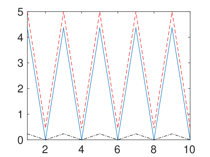
In this example, we will sometimes have one agent using an old dual value for some period of time, and we denote this value by ; its value only changes when we write in the pseudocode in Algorithm 3. Otherwise, does not update with . Similarly, the values of and only change when explicitly updated below and operations listed sequentially below actually occur sequentially so that the agents are updating at different times. To highlight the impact of asynchrony in the dual variable, each agent always uses the most recent state of the other agent in its computations, i.e., and . Then there is no disagreement about state values in the network and superscript indices are therefore omitted. For clarity, we write each argument of and out explicitly, including specifying which dual variable is being used. To simplify notation, timestamps are omitted in the pseudocode in Algorithm 3.
We have so that using the stepsize bounds in Theorems 1 and 2 we select and . This example consists of alternating between two modes, shown in Algorithm 3 where the dual update law in the cloud is represented by the symbol .
Oscillations are shown in Figure 2 where we plot the primal and dual trajectories of a simulation implementing Algorithm 3. Both states and the dual variable oscillate in a non-decaying fashion, indicating that Algorithm 2 is not converging at all. We note here that synchronizing the dual variable in this example does indeed lead to convergence, indicating that the asynchrony of the dual values is the source of oscillations and that Assumption 6.d is a necessary condition for convergence in Algorithm 2.
VII Simulation Results
| Agent Number | Start NodeEnd Node | Edges Traversed |
|---|---|---|
| , , | ||
| , , | ||
| , , , | ||
| , , | ||
| , , , , | ||
| , , | ||
| , , , | ||
| , |
We now present simulation results for Algorithm 2. We first discuss the problem to be solved and then cover our implementation. We then present numerical results that demonstrate convergence of Algorithm 2 on the cloud-based system and the tradeoff between convergence rate and accuracy that is induced by the Tikhonov regularization of .
VII-A Problem Overview
We consider a problem of routing flows through a network consisting of nodes and edges, representing, e.g., traffic flow or sending data across a communication network, and each agent’s decision variable is the flow rate of its data through the network, which is depicted in Figure 3. The nodes of the network are not the agents themselves, but, instead, the agents are users of the network attempting to route traffic between certain pairs of these nodes. The starting points, ending points, and edges which comprise the path traversed by each flow are listed in Table I.
We define the set to be the indices of the edges in the network. The cost of each agent is , and we have selected for all . The network also has an associated congestion cost , where
| (94) |
defines the network’s adjacency matrix .
Each edge in the network is subject to capacity constraints, expressed by requiring , where for all . In addition, each flow rate is confined to , giving . To demonstrate the effects of different values of and , three simulation runs were run: the first with , the second with , and the third with . By sweeping and across three orders of magnitude, we demonstrate the speed-accuracy tradeoff discussed in Remark 3. For each , we take , and we take for each pair.
VII-B Implementation and Numerical Results
The implementation of the above problem allowed as many quantities as possible to be random to demonstrate asynchronous behavior. The time between cloud updates was a random integer chosen from the range to (inclusive) with uniform probability, and this number represents the number of ticks of the virtual clock between and . At each tick of , each agent computed a state update with probability for all agents.
The communication graph at each tick of was an Erdős-Rényi graph [30, Chapter 5], which is a random graph wherein each edge appears with some probability independently of all other edges. We chose , so that at each time we had the graph , where for all and in each other’s essential neighborhoods. The communication graph in this case was undirected so that means that agent sends its state to agent at time , and vice versa. All transmissions are received instantaneously. The times at which the agents sent their states to the cloud were chosen to be randomly generated times between and which were uniformly distributed and independent of all communications and computations.
Each of the three simulation runs was run until it converged. In Figure 4 we see three pairs of curves: the uppermost pair corresponds to , the middle pair corresponds to , and the lowest pair corresponds to . Each pair plots the unregularized primal error for each run using lines, and the regularized primal error is plotted using shapes. Figure 5 similarly shows the regularized and unregularized dual errors, and , using lines and shapes, respectively, for each choice of regularization parameters.
| Value of | Final reg. error | Final unreg. error | Max final value |
|---|---|---|---|
| and | of | ||
Figure 4 shows that all error curves initially increase, following which they decrease at different rates, with larger regularization parameters clearly leading to faster decreases in error. The final primal errors for each simulation run are given in Table II, where we see that all three runs numerically converge almost exactly to . We also see that smaller regularization parameters decrease final primal errors, as predicted by Remark 3.
Figure 5 shows behavior in the dual space similar to that shown in Figure 4. All curves appear to decrease monotonically, with larger values of and clearly showing a faster rate of decrease. And as with the primal space, one finds that larger regularization parameters lead to larger errors in the dual space; final dual error values are shown in Table III wherein one finds that all three runs virtually exactly reach and, indeed, decreasing and decreases the final dual error.
| Value of | Final reg. error | Final unreg. error |
|---|---|---|
| and | ||
We see in Figures 4 and 5 that increasing the regularization parameters leads to faster convergence, and this same phenomenon was observed numerically in [26]. However, a key numerical difference between our results and some of those in earlier works, e.g., [19] and [20], is the initial increase in distance to the optimum seen in Figure 4. This increase is unavoidable due to the agents sharing information asynchronously and is typical in simulation runs of Algorithm .
VIII Conclusion
An asynchronous multi-agent optimization algorithm for constrained problems was presented. It was shown that the dual variable must be kept synchronized across the agents, though their primal updates can occur independently and with arbitrary timing. The method presented used a Tikhonov regularization and a multi-agent gradient projection method to approximately find saddle points of the regularized Lagrangian asynchronously.
References
- [1] M. Khan, G. Pandurangan, and V. Kumar, “Distributed algorithms for constructing approximate minimum spanning trees in wireless sensor networks,” Parallel and Distributed Systems, IEEE Transactions on, vol. 20, no. 1, pp. 124–139, Jan 2009.
- [2] N. Trigoni and B. Krishnamachari, “Sensor network algorithms and applications Introduction,” Philosophical Transactions of the Royal Scoeity A - Mathematical, Physical, and Engineering Sciences, vol. 370, no. 1958, SI, pp. 5–10, Jan 2012.
- [3] J. Cortes, S. Martinez, T. Karatas, and F. Bullo, “Coverage control for mobile sensing networks,” in Robotics and Automation, 2002. Proceedings. ICRA’02. IEEE International Conference on, vol. 2. IEEE, 2002, pp. 1327–1332.
- [4] M. Rabbat and R. Nowak, “Distributed optimization in sensor networks,” in Information Processing in Sensor Networks (ISPN), 2004. Third International Symposium on, April 2004, pp. 20–27.
- [5] D. E. Soltero, M. Schwager, and D. Rus, “Decentralized path planning for coverage tasks using gradient descent adaptive control,” The International Journal of Robotics Research, 2013.
- [6] P. Vytelingum, T. D. Voice, S. D. Ramchurn, A. Rogers, and N. R. Jennings, “Agent-based micro-storage management for the smart grid,” in Proceedings of the 9th International Conference on Autonomous Agents and Multiagent Systems: volume 1-Volume 1. International Foundation for Autonomous Agents and Multiagent Systems, 2010, pp. 39–46.
- [7] S. Caron and G. Kesidis, “Incentive-based energy consumption scheduling algorithms for the smart grid,” in Smart Grid Communications (SmartGridComm), 2010 First IEEE International Conference on, Oct 2010, pp. 391–396.
- [8] F. Kelly, A. Maulloo, and D. Tan, “Rate control in communication networks: shadow prices, proportional fairness and stability,” in Journal of the Operational Research Society, vol. 49, 1998.
- [9] M. Chiang, S. Low, A. Calderbank, and J. Doyle, “Layering as optimization decomposition: A mathematical theory of network architectures,” Proceedings of the IEEE, vol. 95, no. 1, pp. 255–312, Jan 2007.
- [10] D. Mitra, Wireless and Mobile Communications. Boston, MA: Springer US, 1994, ch. An Asynchronous Distributed Algorithm for Power Control in Cellular Radio Systems, pp. 177–186.
- [11] D. P. Bertsekas and J. N. Tsitsiklis, Parallel and Distributed Computation: Numerical Methods. Upper Saddle River, NJ, USA: Prentice-Hall, Inc., 1989.
- [12] D. P. Bertsekas, J. N. Tsitsiklis, D. P. Bertsekas, and J. N. Tsitsiklis, “Convergence rate and termination of asynchronous iterative algorithms,” in In Proceedings of the Int. Conf. on Supercomputing. ACM, 1989, pp. 461–470.
- [13] D. P. Bertsekas, “Distributed asynchronous computation of fixed points,” Mathematical Programming, vol. 27, no. 1, pp. 107–120, 1983.
- [14] D. Chazan and W. Miranker, “Chaotic relaxation,” Linear Algebra and its Applications, vol. 2, no. 2, pp. 199 – 222, 1969.
- [15] G. M. Baudet, “Asynchronous iterative methods for multiprocessors,” J. ACM, vol. 25, no. 2, pp. 226–244, Apr. 1978.
- [16] R. Olfati-Saber and R. M. Murray, “Consensus problems in networks of agents with switching topology and time-delays,” Automatic Control, IEEE Transactions on, vol. 49, no. 9, pp. 1520–1533, 2004.
- [17] M. Zhu and S. Martinez, “On distributed convex optimization under inequality and equality constraints,” IEEE Transactions on Automatic Control, vol. 57, no. 1, pp. 151–164, Jan 2012.
- [18] S. Boyd, A. Ghosh, B. Prabhakar, and D. Shah, “Randomized gossip algorithms,” IEEE/ACM Trans. Netw., vol. 14, no. SI, pp. 2508–2530, Jun. 2006.
- [19] S. Boyd, N. Parikh, E. Chu, B. Peleato, and J. Eckstein, “Distributed optimization and statistical learning via the alternating direction method of multipliers,” Found. Trends Mach. Learn., vol. 3, no. 1, pp. 1–122, Jan. 2011.
- [20] R. Zhang and J. T. Kwok, “Asynchronous distributed admm for consensus optimization.” in ICML, 2014, pp. 1701–1709.
- [21] D. P. Bertsekas, A. E. Ozdaglar, and A. Nedić, Convex analysis and optimization, ser. Athena scientific optimization and computation series. Belmont, Massachusetts: Athena Scientific, 2003.
- [22] H. W. Kuhn and A. W. Tucker, “Nonlinear programming,” in Proceedings of the Second Berkeley Symposium on Mathematical Statistics and Probability. Berkeley, Calif.: University of California Press, 1951, pp. 481–492.
- [23] F. Facchinei and J.-S. Pang, Finite-dimensional variational inequalities and complementarity problems. Springer Verlag, 2003, vol. 1 and 2.
- [24] H. Uzawa, “Iterative methods in concave programming,” Studies in Linear and Non-Linear Programming, pp. 20–27, 1958.
- [25] M. T. Hale, A. Nedić, and M. Egerstedt, “Cloud-based centralized/decentralized multi-agent optimization with communication delays,” in 2015 54th IEEE Conference on Decision and Control (CDC), Dec 2015, pp. 700–705.
- [26] J. Koshal, A. Nedić, and U. V. Shanbhag, “Multiuser optimization: Distributed algorithms and error analysis,” SIAM Journal on Optimization, vol. 21, no. 3, pp. 1046–1081, 2011.
- [27] A. Bakushinskii and B. Polyak, “Solution of variational inequalities,” Doklady Akademii Nauk SSSR, vol. 219, 1974.
- [28] D. E. Comer, Internetworking with TCP/IP, Volume 1: Principles, Protocols, and Architectures, Fourth Edition, 4th ed. Upper Saddle River, NJ, USA: Prentice Hall PTR, 2000.
- [29] B. T. Poljak, Introduction to optimization. Optimization Software, 1987.
- [30] M. Mesbahi and M. Egerstedt, Graph theoretic methods in multiagent networks. Princeton University Press, 2010.