Stochastic difference equations with the Allee effectThanks: E. Braverman is a corresponding author, e-mail maelena@ucalgary.ca.

Abstract.

For a truncated stochastically perturbed equation $x_{n+1}=\max\{f(x_{n})+l\chi_{n+1},0\}$ with $f(x)<x$ on $(0,m)$ , which corresponds to the Allee effect, we observe that for very small perturbation amplitude $l$ , the eventual behavior is similar to a non-perturbed case: there is extinction for small initial values in $(0,m-\varepsilon)$ and persistence for $x_{0}\in(m+\delta,H]$ for some $H$ satisfying $H>f(H)>m$ . As the amplitude grows, an interval $(m-\varepsilon,m+\delta)$ of initial values arises and expands, such that with a certain probability, $x_{n}$ sustains in $[m,H]$ , and possibly eventually gets into the interval $(0,m-\varepsilon)$ , with a positive probability. Lower estimates for these probabilities are presented. If $H$ is large enough, as the amplitude of perturbations grows, the Allee effect disappears: a solution persists for any positive initial value.

Key words and phrases:

stochastic difference equations, Allee effect, a.s. persistence, a.s. low density, population dynamics

1991 Mathematics Subject Classification

Primary: 39A50, 37H10; Secondary: 93E10, 92D25.

Elena Braverman

Dept. of Math. and Stats., University of Calgary, 2500 University Drive N.W., Calgary, AB, Canada T2N 1N4

and Alexandra Rodkina

Department of Mathematics, the University of the West Indies, Mona Campus, Kingston, Jamaica

(Communicated by … )

1. Introduction

Difference equations can describe population dynamics models, and, if there is no compensation for low population size, i.e. the stock recruitment is lower than mortality, the species goes to extinction, unless the initial size is large enough. This phenomenon was introduced in [1], see also [6, 20]. It is called the Allee effect after [1] and can be explained by many factors: problems with finding a mate, deficiency of group defense or/and social functioning for low population densities. If the initial population size is small enough (is in the Allee zone) then the population size tends to zero as the time grows and tends to infinity. Even a small stochastic perturbation which does not tend to zero, significantly changes the situation: due to random immigration, there are large enough values of the population size for some large times even in the Allee zone, due to this occasional immigration. Thus, instead of extinction, we explore eventual low-density behavior, as well as essential persistence and solution bounds. Results on permanence of solutions for stochastic difference equations, including boundedness and persistence, were recently reviewed in [21]. For recent results on asymptotic behavior of stochastic difference equations also see [2, 3, 4, 5, 10, 11, 13, 14, 17, 18, 19, 22] and the whole issue of Journal of Difference Equations and Applications including [21].

The influence of stochastic perturbations on population survival, chaos control and eventual cyclic behavior was investigated in [9, 10, 11]. It was shown that the chaotic behavior could be destroyed by either a positive deterministic [9] or stochastic noise with a positive mean [10, 11]; instead of chaos, there is an attractive two-cycle.

Certainly, stochastic perturbations, applied formally, can lead to negative size values. To avoid this situation, we consider the truncated stochastic difference equation

x_{n+1}=\max\bigl\{f(x_{n})+l\chi_{n+1},0\bigr\},\quad x_{0}>0,\quad n\in\mathbb{N}.

(1)

Here $f$ is a function with a possible Allee zone, for example,

x_{n+1}=\frac{Ax_{n}^{2}}{B+x_{n}}e^{r(1-x_{n})},

(2)

described in [12] and

x_{n+1}=\frac{Ax_{n}}{B+(x_{n}-T)^{2}},

(3)

considered in [15, 16]; see [6] for the detailed outline of models of the Allee effect.

It is well known that, without a stochastic perturbation, if $f(x)$ is a function such that $0<f(x)<x$ for $x\in(0,m)$ and $f(x)>m$ for $x>m$ , the eventual behavior of a solution depends on the initial condition: if $0<x_{0}<m$ , then the solution tends to zero (goes to extinction), if $x_{0}>b$ then the solution satisfies $x_{n}>m$ , i.e. persists. Sometimes high densities also lead to extinction, as in (2) and (3), we can only claim that $f(x)>m$ for $x\in(m,H)$ and conclude persistence for $x_{0}\in(m,H)$ . However, the situation changes for (1) with a stochastic perturbation: for example, even if $f$ has an Allee zone, the eventual expectation of a solution exceeds a positive number depending on $l$ and the distribution of $\chi$ . Nevertheless, this effect is due to immigration only, and we will call this type of behavior blurred extinction, or eventual low density. In the present paper, we use some ideas developed in [8] for models with a randomly switching perturbation.

Significant interest to discrete maps is stimulated by complicated types of behavior exhibited even by simple maps. In particular, for (2) with $r$ large enough, whatever a positive initial value is, the chaotic solution can take values in the interval $(0,\varepsilon)$ for any small $\varepsilon>0$ . Then, in practical applications the dynamics is not in fact chaotic but leads to eventual extinction as the positive density cannot be arbitrarily low. Nevertheless, if the range is separated from zero, for some maps there is an unconditional survival (persistence), independently of a positive initial value.

In this note, we are mostly interested in the maps $f$ with survival for certain initial values and an Allee zone: if $x_{0}$ is small enough, then the solution of (1) with $l=0$ tends to zero, and there is an interval $[a,H]\subset(0,\infty)$ which $f$ maps into itself. The main results of the paper are the following:

(1)

If in (1) the value of $l$ is small enough, the dynamics is similar to the non-stochastic case: blurred extinction (low density) for small $x_{0}$ and persistence for $x_{0}$ in a certain interval.
(2)

If $l>0$ is large enough then, under some additional assumptions, there is an unconditional survival.
(3)

If the non-perturbed system has several attraction zones then for any initial condition, the solution can become persistent with large enough lower bound, whenever $l$ is large enough.

The paper is organized as follows. After describing all relevant assumptions and notations in Section 2, we state that for perturbations small enough, there is the same Allee effect as in the deterministic case, in Section 3. The result that there may exist large enough perturbation amplitudes ensuring survival for any positive initial condition, is also included in Section 3. Further, Section 4 deals with the case when, for certain initial conditions, both persistence and low-density behavior are possible, with a positive probability, while for other initial conditions, a.s. persistence or a.s. low-density behavior is guaranteed. For initial values leading to different types of dynamics, lower bounds for probabilities of each types of dynamics are developed in Section 4. The case when the deterministic equation has more than 2 positive fixed point, is considered in Section 5. The results are illustrated with numerical examples in Section 6, and Section 7 involves a short summary and discussion.

2. Preliminaries

Let $(\Omega,{\mathcal{F}},(\mathcal{F}_{n})_{n\in\mathbb{N}},{\mathbb{P}})$ be a complete filtered probability space. Let $\chi:=(\chi_{n})_{n\in\mathbb{N}}$ be a sequence of independent random variables with the zero mean. The filtration $(\mathcal{F}_{n})_{n\in\mathbb{N}}$ is supposed to be naturally generated by the sequence $(\chi_{n})_{n\in\mathbb{N}}$ , namely $\mathcal{F}_{n}=\sigma\left\{\chi_{1},\dots,\chi_{n}\right\}$ .

In the paper we assume that stochastic perturbation $\chi$ in the equation (1) satisfies the following assumption

Assumption 1.

$(\chi_{n})_{n\in\mathbb{N}}$ is a sequence of independent and identically distributed continuous random variables with the density function $\phi(x)$ , such that

\phi(x)>0,\quad x\in(-1,1),\quad\phi(x)\equiv 0,\quad x\notin[-1,1].

We use the standard abbreviation “a.s.” for the wordings “almost sure” or “almost surely” with respect to the fixed probability measure $\mathbb{P}$ throughout the text. A detailed discussion of stochastic concepts and notation may be found in, for example, Shiryaev [23].

Everywhere below, for each $t\in[0,\infty)$ , we denote by $[t]$ the integer part of $t$ .

Before we proceed further, let us introduce assumptions on the function $f$ in (1).

Assumption 2.

$f:(0,\infty)\to(0,\infty)$ is continuous, $f(0)=0$ , and there exist positive numbers $a$ and $H$ , $a<H$ , such that

(i)

$f^{H}:=\max_{x\in[0,H]}f(x)<H$ ;
(ii)

$f(x)>f(a)>a,\quad x\in(a,H]$ .

So far we have not supposed that there is an Allee zone, where for small initial values, a solution of the non-perturbed system tends to zero. This is included in the next condition.

Assumption 3.

There is a point $b_{1}>0$ such that $f(x)<x$ and $f(x)\leq f(b_{1})$ for $x\in(0,b_{1})$ .

3. Unconditional Persistence and Low-Density Behavior

In this section, we consider the case when the type of perturbation and the initial condition allow us to predict a.s. the eventual behavior of the solution. Lemma 3.1 indicates a small initial interval, where the Allee effect is observed, for small enough perturbations. Lemma 3.2 presents the range of initial conditions which guarantee permanence of solutions, for $l$ small enough. However, for large enough $l$ and appropriate $f$ , the Allee effect completely disappears under a stochastic perturbation, see Theorem 3.3.

Lemma 3.1.

Let Assumptions 1 and 3 hold, $f(b_{1})<b_{1}$ . Let $x_{n}$ be a solution of equation (1) with

l\leq b_{1}-f(b_{1})

(4)

and $x_{0}\in[0,b_{1}]$ . Then, $x_{n}\in[0,b_{1}]$ for all $n\in{\mathbb{N}}$ .

Proof.

For $x_{0}\in[0,b_{1}]$ , we have $f(x_{0})\leq f(b_{1})$ and, a.s. on $\Omega$ ,

x_{1}=f(x_{0})+l\chi_{1}\leq f(b_{1})+l\leq f(b_{1})+b_{1}-f(b_{1})\leq b_{1}.

Similarly, the induction step implies $x_{n}\in[0,b_{1}]$ for all $n\in{\mathbb{N}}$ , a.s. ∎

Let us introduce the function

F(x)=f(x)-x,\quad x\in[0,\infty).

(5)

Remark 1.

Assumption 3 holds for non-decreasing $f$ such that $f(x)<x$ for $x$ small enough. In this case, once it is satisfied for a given $b_{1}>0$ , this is also true for any $b\in(0,b_{1})$ . For example, if $f(x)<x$ on $(0,b_{2})$ and $f(b_{2})=b_{2}$ , we can take any $b_{1}<b_{2}$ in Assumption 3. Then, the continuous function $F(x)=f(x)-x$ is negative on $(0,b_{2})$ and vanishes at the end of the interval, so it attains its minimum at a point inside the interval. Moreover, if Assumptions 2 and 3 hold, we have $F(a)>a$ , and also there is a minimum of $F(x)$ on $[0,a]$ attained on $(0,a)$ at a point $b$ :

b=\min\left\{\beta>0:F(\beta)=\min_{x\in[0,a]}F(x)\right\}.

(6)

Lemma 3.2.

Let Assumptions 1 and 2 hold, and $(x_{n})$ be a solution of equation (1), with the noise amplitude $l$ satisfying

l<\min\{H-f^{H},\,\,F(a)\},

(7)

with an arbitrary initial value $x_{0}\in(0,H)$ . Then, a.s., for all $n\in\mathbb{N}$ ,

(i)

$x_{n}\leq H$ ;
(ii)

if in addition $x_{0}\in(a,H)$ then $x_{n}\in(a,H)$ .

Proof.

If, for some $\omega\in\Omega$ and $n\in\mathbb{N}$ , we have $x_{n}(\omega)\leq H$ , then by Assumption 2, (i), and (7),

x_{n+1}(\omega)=f(x_{n}(\omega))+l\chi_{n+1}(\omega)\leq f^{H}+l<H.

If, for some $\omega\in\Omega$ and $n\in\mathbb{N}$ , we also have $x_{n}(\omega)\in(a,H]$ , then by Assumption 2, (ii), and (7),

x_{n+1}(\omega)=f(x_{n}(\omega))+l\chi_{n+1}(\omega)>f(a)-l=f(a)-a+a-l>l+a-l=a.

∎

Remark 2.

Lemma 3.2 implies persistence of solutions with initial values $x_{0}\in(a,H)$ .

Theorem 3.3.

Let Assumptions 1 and 2 hold, $b$ be defined in (6), $(x_{n})$ be a solution of equation (1) with $l$ satisfying (7) and

l>b-f(b)=-F(b),

(8)

and $x_{0}\in(0,H)$ . Then, a.s., $x_{n}$ eventually gets into the interval $(a,H)$ and stays there.

Proof.

By Lemma 3.2, it is sufficient to prove that $x_{n}\in(a,H)$ for some $n\in{\mathbb{N}}$ , a.s. Let $\delta>0$ satisfy $l>b-f(b)+\delta$ (in particular, we can take $\delta=\alpha(l-b+f(b))$ for any $\alpha\in(0,1)$ ). We define

p_{1}:=\mathbb{P}\left\{\omega\in\Omega:\chi(\omega)\in\left(\frac{b-f(b)+\delta}{l},1\right)\right\},\quad K:=\left[\frac{a}{\delta}\right]+1.

(9)

By Lemma 3.2 we only have to consider the case $x_{0}\in(0,a]$ . Let us note that for any $x_{n}\in(0,a]$ and $\displaystyle\chi_{n+1}\in\left(\frac{b-f(b)+\delta}{l},1\right)$ , we have

\begin{split}x_{n+1}=f(x_{n})+l\chi_{n+1}\geq&f(x_{n})-x_{n}+x_{n}+l\frac{b-f(b)+\delta}{l}\\ \geq&f(b)-b+x_{n}+b-f(b)+\delta=x_{n}+\delta.\end{split}

By Assumption 1, $p_{1}>0$ , moreover, the probability

p_{K}:=\mathbb{P}\left\{\omega\in\Omega:\chi_{i}(\omega)\in\left(\frac{b-f(b)+\delta}{l},1\right)~~i=1,\dots,K\right\}=p_{1}^{K}>0.

(10)

Thus, the probability

\begin{split}p_{out}:=\mathbb{P}\left\{\omega\in\Omega:\chi_{j}(\omega)\in\left[-1,\frac{b-f(b)+\delta}{l}\right]\mbox{~for some~~}j\in\{1,\dots,K\}\right\}=1-p_{1}^{K}\in(0,1).\end{split}

If all $\chi_{i}$ , $i=j+1,j+2,j+K$ , are in $\displaystyle\left(\frac{b-f(b)+\delta}{l},1\right)$ , then

x_{j+1}\geq x_{j}+\delta,~x_{j+2}\geq x_{j+1}+\delta\geq x_{j}+2\delta,~~\dots~,x_{j+K}\geq x_{j}+K\delta>a.

By Lemma 3.2, it is sufficient to show that the probability $p_{s}=0$ , where

\begin{split}p_{s}:={\mathbb{P}}\left\{\omega\in\Omega:\mbox{~among any $K$ successive $j$ ~, there is~}\chi_{j}(\omega)\in\left[-1,\frac{b-f(b)+\delta}{l}\right]\right\}=0.\end{split}

Let us take some $\varepsilon>0$ and prove that $p_{s}<\varepsilon$ . Among any $K$ successive $j$ , there is $\chi_{j}$ in the above interval with probability $p_{out}<1$ . In particular, there is such $\chi_{j}$ among $j=1,\dots,K$ , with probability $p_{out}$ , as well as among $j=K+1,\dots,2K$ , and in any of non-intersecting sets $j=nK,nK+1,\dots,(n+1)K-1$ , $n=0,\dots m-1$ . The probability that there is $\chi_{j}$ in the above interval among any $K$ successive $\chi_{j}$ among $j=1,\dots,mK-1$ , is $p_{out}^{m}$ , and $p_{s}\leq p_{out}^{m}$ . Since $p_{out}^{m}<\varepsilon$ as soon as $m>\ln\varepsilon/\ln(p_{out})$ , we conclude that $p_{s}=0$ , which completes the proof. ∎

Corollary 1.

Under the assumptions of Theorem 3.3, if in addition we assume $f(x)<x-l$ for $x>H$ , then, for any initial condition $x_{0}\in[0,\infty)$ , all solutions eventually belong to the interval $(a,H)$ .

4. Dynamics Depending on Perturbations (the case $l<b-f(b)$ )

In this section we assume that

l<b-f(b)=-F(b),

(11)

where $b$ is defined in (6), and $f$ corresponds to the system with an Allee effect. As we assume an upper bound for the perturbation, the dynamics is expected to be dependent on the initial condition: low density if the initial condition is small enough and sustainable (persistent) for a large enough initial condition. We recall that a solution $(x_{n})$ is persistent if there exist $n_{0}\in{\mathbb{N}}$ and $a>0$ such that $x_{n}>a$ for any $n\geq n_{0}$ .

In a non-stochastic case, if the system exhibits the Allee effect, then for a small initial condition, the solution tends to zero. However, in the case of both truncation and stochastic perturbations satisfying Assumption 1, the expectation of $x_{n}$ exceeds a certain positive number. The density function $\phi(x)$ is positive, thus

\alpha:=\int_{0}^{1}x\phi(x)~dx>0.

(12)

Lemma 4.1.

Suppose that Assumption 1 holds and $f:(0,\infty)\to(0,\infty)$ is a continuous function. Then the expectation of the solution $(x_{n})$ of (1) is not less than $\alpha$ defined in (12).

Proof.

From (1), $x_{n}\geq\max\{l\chi_{n},0\}$ , thus the expectation of $x_{n}$ is not less than

\int_{-1}^{1}l\max\{x,0\}\phi(x)~dx=\int_{-1}^{0}0\,\phi(x)~dx+\int_{0}^{1}x\phi(x)~dx=\alpha,

which concludes the proof. ∎

4.1. A.s. persistence and a.s. low density areas

Suppose that Assumptions 2,3 hold with $b_{1}\geq b$ , where $b$ is denoted in (6) and $l$ satisfies (7). Then we can introduce positive numbers

u_{l}:=\sup\{u<a:F(u)<l\}

(13)

and

v_{l}:=\inf\{v>b:F(v)>-l\},

(14)

where $F$ is defined in (5).

Theorem 4.2.

Suppose that Assumptions 1 - 3 hold with $b_{1}\geq b$ , where $b$ is denoted in (6) and $l$ satisfies (7), (11). Let $(x_{n})$ be a solution to (1) with an arbitrary initial value $x_{0}\in[0,H]$ . Let $u_{l}$ be defined as in (13) and $v_{l}$ be defined as in (14). Then the following statements are valid.

(i)

$b<v_{l}<u_{l}<a$ .
(ii)

$F(u_{l})=l$ , $F(v_{l})=-l$ , $F(x)\geq l$ , for $x\in(u_{l},a)$ , $F(x)\leq-l$ , for $x\in(b,v_{l})$ .
(iii)

If $x_{0}\in(0,v_{l})$ , there exists $n_{1}\in{\mathbb{N}}$ such that $x_{n}\in[0,b]$ a.s. for $n\geq n_{1}$ .
(iv)

If $x_{0}\in(u_{l},H)$ then $x$ persists a.s.; moreover, there exists $n_{2}\in{\mathbb{N}}$ such that $x_{n}\in[a,H]$ a.s. for $n\geq n_{2}$ .

Proof.

Since

b\in\{u<a:f(u)-u<l\},\quad a\in\{v>b:v-f(v)<l\},

both sets in (13) and (14) are non-empty and $u_{l}\leq a$ , $v_{l}\geq b$ . By continuity of $f$ and Assumptions 2,3 we have

u_{l}<a,\quad v_{l}>b,\quad F(u_{l})=l,\quad F(v_{l})=-l.

So $u_{l}\neq v_{l}$ ,

v_{l}\in\{u<a:F(u)<l\}\implies v_{l}<u_{l},

which completes the proof of (i)-(ii).

(iii) Define

\Delta_{l}(y):=\inf_{x\in[b,y]}\{x-f(x)-l\}.

Note that

\Delta_{l}(b)=b-f(b)-l>0,\quad\Delta_{l}(v_{l})=0,

and the function $\Delta_{l}:[b,v_{l}]\to[b-f(b)-l,\,0]$ is non-increasing. Then, for each $x_{0}\in(b,v_{l})$ and each $x\in(b,x_{0})$ , we have

\Delta_{l}(x_{0})\leq\Delta_{l}(x),\quad x-f(x)-l\geq\Delta_{l}(x).

So, a.s.,

x_{1}=f(x_{0})+l\chi_{1}\leq f(x_{0})+l\leq f(x_{0})+x_{0}-f(x_{0})-\Delta_{l}(x_{0})=x_{0}-\Delta_{l}(x_{0}).

If $x_{1}\leq b$ we stop. If $x_{1}>b$ , we have, a.s.,

x_{2}=f(x_{1})+l\chi_{2}\leq f(x_{1})+l\leq f(x_{1})+x_{1}-f(x_{1})-\Delta_{l}(x_{1})\leq x_{0}-\Delta_{l}(x_{0})-\Delta_{l}(x_{1})\leq x_{0}-2\Delta_{l}(x_{0}).

Thus, after at most $K$ steps, where

K=\left[\frac{v_{l}-b}{\Delta_{l}(x_{0})}\right]+1,

$x_{n}$ gets into the interval $(0,b)$ and by Lemma 3.1 stays there a.s.

(iv) Define

\tilde{\Delta}_{l}(y):=\inf_{x\in[y,a]}\{f(x)-x-l\},

and note that

\tilde{\Delta}_{l}(a)=f(a)-a-l>0,\quad\tilde{\Delta}_{l}(v_{l})=0,

and the function $\tilde{\Delta}_{l}:[v_{l},a]\to[0,\,f(a)-a-l]$ is non-decreasing. Then, for each $x_{0}\in(u_{l},a)$ and each $x\in(x_{0},a)$ , we have

\tilde{\Delta}_{l}(x_{0})\leq\tilde{\Delta}_{l}(x),\quad f(x)-x-l\geq\tilde{\Delta}_{l}(x).

So, a.s.,

x_{1}=f(x_{0})+l\chi_{1}\geq f(x_{0})-l\geq f(x_{0})+\tilde{\Delta}_{l}(x_{0})-f(x_{0})+x_{0}=x_{0}+\tilde{\Delta}_{l}(x_{0}).

If $x_{1}\geq a$ we stop. If $x_{1}<a$ , we have, a.s.,

x_{2}=f(x_{1})+l\chi_{2}\geq f(x_{1})-l\geq f(x_{1})+\tilde{\Delta}_{l}(x_{1})-f(x_{1})+x_{1}\geq x_{0}+\tilde{\Delta}_{l}(x_{0})+\tilde{\Delta}_{l}(x_{1})\geq x_{0}+2\tilde{\Delta}_{l}(x_{0}).

Thus, after at most $K$ steps, where

K=\left[\frac{a-u_{l}}{\tilde{\Delta}_{l}(x_{0})}\right]+1,

$x_{n}$ gets into the interval $(a,H)$ and stays there, a.s., by Lemma 3.2. ∎

4.2. Mixed behavior

So far we have considered the areas starting with which the solution is guaranteed to sustain (and be in $[a,H]$ ) or to stay in the neighbourhood $[0,b]$ of zero. Let us consider a more complicated case when a solution can either eventually persist or eventually belong to $[0,b]$ . We single out intervals starting with which a solution can change domains of attraction, switch between persistence and low-density behavior. In particular, we obtain lower bounds for probabilities that eventually $x_{n}\in[a,H]$ and $x_{n}\in[0,b]$ .

As everywhere above, in this subsection we assume that Assumptions 1-3 and conditions (7), (11) hold. Based on this, we can define

\beta_{l}=\inf\{b<x<a:F(x)>l\},\quad\alpha_{l}=\sup\{b<x<a:F(x)<-l\}.

(15)

Note that, since $F(a)>l$ , $F(b)<-l$ , and $F$ is continuous, both sets in the right-hand-sides of formulae in (15) are non-empty.

Let $u_{l}$ and $v_{l}$ be defined as in (13) and (14), respectively. Note that

v_{l}<\beta_{l}\leq u_{l},\quad v_{l}\leq\alpha_{l}<u_{l},

and

\max_{x\in[b,\beta_{l}]}F(x)\leq l,\quad\min_{x\in[\alpha_{l},a]}F(x)\geq-l.

The points $a,b,u_{l},v_{l},\alpha_{l},\beta_{l}$ are illustrated in Figure 1.

Refer to caption — Figure 1. An illustration of the points $a,b,u_{l},v_{l},\alpha_{l},\beta_{l}$ in the two cases: (left) $\alpha_{l}<\beta_{l}$ and (right) $\alpha_{l}>\beta_{l}$ .

Remark 3.

It is possible that $\alpha_{l}>\beta_{l}$ , see Example 1 and Fig. 1, right. However, as $F$ is continuous, $F(b)<-l$ , $F(\beta_{l})=l$ , $F(\alpha_{l})=-l$ , $F(a)>l$ , the inequality $\alpha_{l}>\beta_{l}$ immediately implies that there are at least 3 fixed points of $f$ on $(b,a)$ . In this case we are able to prove only “essential extinction” for $x_{0}\in(v_{l},\beta_{l})$ and persistence for $x_{0}\in(\alpha_{l},u_{l})$ (see Lemma 4.3 below).

However, if $\alpha_{l}<\beta_{l}$ , for each $x_{0}\in(\alpha,\beta)\subset(\alpha_{l},\beta_{l})$ , a solution persists with a positive probability and also reaches the interval $[0,b]$ with a positive probability. So solutions with the initial value on the non-empty interval $(\alpha_{l},\beta_{l})$ demonstrate mixed behavior (see Corollary 2 below).

Example 1.

Consider (1) with

f(x)=\left\{\begin{array}[]{ll}\displaystyle\frac{3x}{3+(x-2)^{2}},&0\leq x\leq 1;\\ \\ x-\sin(\pi(x-1))-\frac{1}{4},&1<x\leq 5;\\ \\ \displaystyle\frac{8.55x}{8+(x-6)^{2}},&5\leq x.\end{array}\right.

We can take $a=5.2$ , $f(a)\approx 5.4286$ , $H=7$ , $f^{H}<6.8$ , $f(H)=6.65>a$ , $F(H)=-0.35$ . Here the minimum $-\frac{5}{4}$ of $F(x)$ is first attained at $b=\frac{3}{2}$ , however, $\displaystyle F\left(\frac{7}{2}\right)=-\frac{5}{4}$ as well. We consider $l<\min\{F(a),H-f^{H},-F(b)\}$ , so we can take $l<\min\{0.2286,0.2,1.25\}$ . Then, it is easy to see that $\alpha_{l}\in(3.5,5.2)$ , $\beta_{l}\in\left(\frac{3}{2},\frac{5}{2}\right)=(1.5,2.5)$ , so $\beta_{l}<\alpha_{l}$ . There are exactly 4 fixed points of $f(x)=x-\sin(\pi(x-1))-1/4$ on $[1,5]$ which are $\arcsin(0.25)/\pi+1$ , $2-\arcsin(0.25)/\pi$ , $\arcsin(0.25)/\pi+3$ , $4-\arcsin(0.25)/\pi$ , and a fixed point $\approx 5.106$ on $(5,5.2)$ .

Let $x_{0}\in(\alpha_{l},u_{l}]$ . Define

A=A(x_{0}):=\min_{x\in[x_{0},u_{l}]}F(x)>-l

(16)

and

p_{1}=p_{1}(x_{0}):=\mathbb{P}\left\{\omega\in\Omega:\chi(\omega)\geq 1-\frac{l+A}{2l}\right\},\quad K_{1}=K_{1}(x_{0}):=\left[\frac{2(u_{l}-x_{0})}{l+A}\right]+1.

(17)

Let $x_{0}\in[v_{l},\beta_{l})$ . Define

B=B(x_{0}):=\max_{x\in[v_{l},x_{0}]}F(x)<l

(18)

and

p_{2}=p_{2}(x_{0}):=\mathbb{P}\left\{\omega\in\Omega:\chi(\omega)\leq-1+\frac{l-B}{2l}\right\},\quad K_{2}=K_{2}(x_{0}):=\left[\frac{2(x_{0}-v_{l})}{l-B}\right]+1.

(19)

Lemma 4.3.

Let Assumptions 1-3 hold and $l$ satisfy conditions (7) and (11), where $b$ is defined as in (6). Let $(x_{n})$ be a solution to (1) with $x_{0}\in[0,H]$ , and $\alpha_{l}$ , $\beta_{l}$ be denoted by (15).

Then the following statements are valid.

(i)

If $x_{0}\in(\alpha_{l},H]$ then the solution $x_{n}$ will eventually get into the interval $[a,H]$ with the persistence probability $P_{p}$ such that

$P_{p}\geq p_{1}^{K_{1}},$

where $p_{1}$ and $K_{1}$ are defined in (17).
(ii)

If $x_{0}\in[0,\beta_{l})$ then the solution $x_{n}$ will eventually get into the interval $[0,b]$ with the “low density” (“essential extinction”) probability $P_{e}$ satisfying

$P_{e}\geq p_{2}^{K_{2}},$

where $p_{2}$ and $K_{2}$ are defined in (19).

Proof.

Let $u_{l}$ and $v_{l}$ be defined by (13), (14), respectively. By Theorem 4.2, it is enough to prove (i) for $x_{0}\in(\alpha_{l},u_{l}]$ and (ii) for $x_{0}\in[v_{l},\beta_{l})$ .

(i) Let $A$ , $K_{1}$ and $p_{1}$ be defined, respectively, as in (16) and (17). We set

\Omega_{k}:=\left\{\omega\in\Omega:\chi_{k}(\omega)\geq 1-\frac{l+A}{2l}\right\},\quad k=1,2,\dots,K_{1},\quad\mathcal{A}:=\bigcap_{k=1}^{K_{1}}\Omega_{k}.

Note that

\mathbb{P}\left[\mathcal{A}\right]=p_{1}^{K_{1}}.

We prove that

For each

\omega\in\mathcal{A}

there exists a number

n\leq K_{1}

, such that

x_{n}(\omega)>u_{l}.

(20)

By (16), $F(x)\geq A>-l$ , for any $x\in[x_{0},u_{l}]$ . Since $\mathcal{A}\subseteq\Omega_{1}$ we have, on $\mathcal{A}$ ,

x_{1}=f(x_{0})+l\chi_{1}=x_{0}+F(x_{0})+l\chi_{1}\geq x_{0}+A+l\left(1-\frac{l+A}{2l}\right)=x_{0}+\frac{l+A}{2}.

Similarly, for each $k=1,2,\dots,K_{2}-1$ , if $x_{k}\in[x_{0},u_{l}]$ , since $\mathcal{A}\subseteq\Omega_{k}$ and $F(x_{k})\geq A>-l$ , we have, on $\mathcal{A}$ ,

x_{k+1}\geq x_{k}+\frac{l+A}{2}.

The set $\mathcal{A}$ can be presented as

\mathcal{A}=\mathcal{A}_{11}\cup\mathcal{A}_{12},\quad\mathcal{A}_{11}\cap\mathcal{A}_{12}=\emptyset,

where

\mathcal{A}_{11}:=\left\{\omega\in\mathcal{A}:x_{1}(\omega)>u_{l}\right\},\quad\mathcal{A}_{12}:=\left\{\omega\in\mathcal{A}:x_{1}(\omega)\in\left(x_{0}+\frac{l+A}{2},\,u_{l}\right]\right\}.

If $\mathbb{P}\left[\mathcal{A}_{12}\right]=0$ , we have, a.s., $\mathcal{A}=\mathcal{A}_{11}$ . So (20) holds a.s. on $\mathcal{A}$ with $n=1$ .

If $\mathbb{P}\left[\mathcal{A}_{12}\right]>0$ , we have, on $\mathcal{A}_{12}$ ,

x_{2}\geq x_{1}+\frac{l+A}{2}\geq x_{0}+2\frac{l+A}{2}.

Presenting $\mathcal{A}_{12}$ in the same way as above,

\mathcal{A}_{12}=\mathcal{A}_{21}\cup\mathcal{A}_{22},\quad\mathcal{A}_{21}\cap\mathcal{A}_{22}=\emptyset,

where

\mathcal{A}_{21}:=\left\{\omega\in\mathcal{A}_{12}:x_{2}(\omega)>u_{l}\right\},\quad\mathcal{A}_{22}:=\left\{\omega\in\mathcal{A}_{12}:x_{2}(\omega)\in\left(x_{0}+2\frac{l+A}{2},\,u_{l}\right]\right\},

we consider again two cases: $\mathbb{P}\left[\mathcal{A}_{22}\right]=0$ and $\mathbb{P}\left[\mathcal{A}_{22}\right]>0$ . If $\mathbb{P}\left[\mathcal{A}_{22}\right]=0$ , we have, a.s., $\mathcal{A}=\mathcal{A}_{11}\cup\mathcal{A}_{21}$ , so (20) holds with $n=1$ on $\mathcal{A}_{11}$ and $n=2$ on $\mathcal{A}_{21}$ . If $\mathbb{P}\left[\mathcal{A}_{22}\right]>0$ we continue the process.

Analogously, if $\mathbb{P}\left[\mathcal{A}_{k-1,2}\right]>0$ , for some $k<K_{1}$ , we set

\mathcal{A}_{k-1,2}=\mathcal{A}_{k1}\cup\mathcal{A}_{k2},\quad\mathcal{A}_{k1}\cap\mathcal{A}_{k2}=\emptyset,

where

\mathcal{A}_{k1}:=\left\{\omega\in\mathcal{A}_{k-1,2}:x_{k}(\omega)>u_{l}\right\},\quad\mathcal{A}_{k2}:=\left\{\omega\in\mathcal{A}_{k-1,2}:x_{k}(\omega)\in\left(x_{0}+k\frac{l+A}{2},\,u_{l}\right]\right\}.

When $\mathbb{P}\left[\mathcal{A}_{k,2}\right]=0$ , we have, a.s., $\mathcal{A}=\cup_{i=1}^{k}\mathcal{A}_{i1}$ , so (20) holds with $n=i$ on $\mathcal{A}_{i1}$ , $i=1,2,\dots,k$ . When $\mathbb{P}\left[\mathcal{A}_{k,2}\right]>0$ , we continue the process. However, by (17), $x_{0}+K_{1}\frac{l+A}{2}>u_{l}$ , so $\mathcal{A}_{K_{1},2}=\emptyset$ . Then $\mathcal{A}$ can be presented as $\cup_{i=1}^{k}\mathcal{A}_{i1}$ where $k$ does not exceed $K_{1}$ . This proves (20), so the solution reaches the interval $[u_{l},H]$ after at most $K_{1}$ steps with a probability at least $p_{1}^{K_{1}}$ . Application of Theorem 4.2, (iv), completes the proof of (i).

Part (ii) can be proved in a similar way. For $B$ , $K_{2}$ and $p_{2}$ defined, respectively, as in (18) and (19), we set

\Gamma_{k}:=\left\{\omega\in\Omega:\chi_{k}(\omega)<-1+\frac{l-B}{2l}\right\},\quad k=1,2,\dots,K_{2},\quad\mathcal{B}:=\bigcap_{k=1}^{K_{2}}\Gamma_{k},

and notice that

\mathbb{P}\left[\mathcal{B}\right]=p_{2}^{K_{2}}.

By (18), $F(x)\leq B<l$ , for any $x\in[v_{l},x_{0}]$ . Then, on $\mathcal{B}$ , if $x_{k}\in[v_{l},x_{0}]$ , $k=1,2,\dots,K_{2}-1$ , we get

x_{k+1}\leq x_{k}-\frac{l-B}{2}.

Noting that $x_{0}-K_{2}\frac{l-B}{2}<v_{l}$ , we show that for each $\omega\in\mathcal{B}$ , there exists a number $n\leq K_{2}$ , such that $x_{n}(\omega)<v_{l}.$ So the solution reaches the interval $[0,v_{l}]$ after at most $K_{2}$ steps with the probability at least $p_{2}^{K_{2}}$ . Application of Theorem 4.2, (iii), completes the proof of (ii). ∎

Remark 4.

Under the assumptions of Lemma 4.3,

(i)

the persistence probability $P_{p}$ and the “low density” probability $P_{e}$ depend on $x_{0}$ ;
(ii)

the number $K_{1}$ indicates the number of steps necessary for a solution $x_{n}$ with the initial value $x_{0}\in(\alpha_{l},u_{l})$ to get into the interval $(u_{l},H]$ . Respectively, $K_{2}$ is the number of steps required for a solution with the initial value $x_{0}\in(v_{l},\beta_{l})$ to get into the interval $(0,v_{l})$ .

Remark 5.

Estimations of probabilities $P_{p}(x_{0})$ and $P_{e}(x_{0})$ are far from being sharp. They can be improved under the assumption that $F$ is increasing, if, on each step, we estimate the new probability to move right $(A+l)/2$ units (respectively, left $(l-B)/2$ units), see Theorem 4.7 and Corollary 4 below.

Corollary 2.

Let the conditions of Lemma 4.3 hold, and $x_{n}$ be a solution of (1) with the initial value $x_{0}\in[0,H]$ .

(i)

If $\alpha\in(\alpha_{l},u_{l})$ , we can estimate the persistence probability $P_{p}(\alpha)$ uniformly for all initial values $x_{0}\in[\alpha,H]$ . Similarly, if $\beta\in(v_{l},\beta_{l})$ we can estimate the “low density” probability $P_{e}(\beta)$ uniformly for all initial values $x_{0}\in[0,\beta]$ .
(ii)

If $\alpha_{l}<\beta_{l}$ , for each $x_{0}\in(\alpha_{l},\beta_{l})$ a solution persists with a positive probability and also reaches the interval $[0,b]$ with a positive probability. For $(\alpha,\beta)\subset(\alpha_{l},\beta_{l})$ , we can find estimation of $P_{p}$ and $P_{e}$ valid for all $x_{0}\in(\alpha,\beta)$ .

Proof.

If $\alpha\in(\alpha_{l},a)$ then $\displaystyle\min_{x\in[\alpha,a]}F(x)>-l$ , and if $\beta\in(b,\beta_{l})$ then $\displaystyle\max_{x\in[b,\beta]}F(x)<l$ .

In order to prove (i), we choose

\begin{split}&A(\alpha):=\min_{x\in[\alpha,u_{l}]}F(x)>-l,\quad B(\beta):=\min_{x\in[v_{l},\beta]}F(x)<l,\\ &p_{1}(\alpha):=\mathbb{P}\left\{\omega\in\Omega:\chi(\omega)\geq 1-\frac{l+A(\alpha)}{2l}\right\},\quad\,\,\,\,K_{1}(\alpha):=\left[\frac{2(u_{l}-\alpha)}{l+A(\alpha))}\right]+1,\\ &p_{2}(\beta):=\mathbb{P}\left\{\omega\in\Omega:\chi(\omega)\leq-1+\frac{l-B(\beta)}{2l}\right\},\quad K_{2}(\beta):=\left[\frac{2(\beta-v_{l})}{l-B(\beta)}\right]+1.\end{split}

Taking any $x_{0}\in[\alpha,u_{l}]$ and following the proof of Lemma 4.3, after at most $K_{1}(\alpha)$ steps we have on $\displaystyle\cap_{i=1}^{K_{1}(\alpha)}\left\{\omega\in\Omega_{i}:\chi_{i}(\omega)\geq 1-(l+A(\alpha))/(2l)\right\}$ :

x_{n}\geq x_{0}+K_{1}(\alpha)\frac{l+A(\alpha)}{2}=\alpha+\left(\left[\frac{2(u_{l}-\alpha)}{l+A(\alpha))}\right]+1\right)\frac{l+A(\alpha)}{2}\geq\alpha+u_{l}-\alpha=u_{l}.

So the persistence probability $P_{p}$ satisfies the first of the two estimates

P_{p}\geq p_{1}(\alpha)^{K_{1}(\alpha)},\quad P_{e}\geq p_{2}(\beta)^{K_{2}(\beta)}.

(21)

A similar estimation can be done for any $x_{0}\in[v_{l},\beta]$ , and the ”low density” probability $P_{e}$ satisfies the second estimate in (21).

Case (ii) follows from case (i), since for any $x_{0}\in(\alpha,\beta)$ , estimations of both probabilities $P_{p}$ and $P_{e}$ in (21) are valid. ∎

The proof of the following Lemma is straightforward and thus will be omitted.

Lemma 4.4.

Let the assumptions of Lemma 4.3 hold.

(1)

The inequality

$|F(x)|<l,\quad x\in(v_{l},u_{l}),$ (22)

is equivalent to $\beta_{l}=u_{l}$ and $\alpha_{l}=v_{l}$ .
(2)

In particular, condition (22) holds if

$f(x_{2})-f(x_{1})>x_{2}-x_{1}\mbox{\rm~ for any ~~ }v_{l}\leq x_{1}<x_{2}\leq u_{l}.$ (23)

Remark 6.

Note that

(i)

$u_{l}$ is a non-decreasing function of $l$ , while $v_{l}$ is a non-increasing function of $l$ . So, for $l_{1}<l_{2}<b$ we have $(v_{l_{1}},u_{l_{1}})\subseteq(v_{l_{2}},u_{l_{2}})$ .
(ii)

$\beta_{l}$ is a non-decreasing function of $l$ , while $\alpha_{l}$ is a non-increasing function of $l$ .
(iii)

If condition (22) holds for some $l=l_{1}$ , it however can fail for some $l=l_{2}<l_{1}$ (see Example 2).
(iv)

If condition (23) holds for some $l=l_{1}$ then (23), and therefore (22), will be fulfilled for all $l=l_{2}<l_{1}$ .

In the following example we demonstrate the case when (22) holds for some $l=l_{1}$ but does not hold for any smaller $l$ .

Example 2.

Consider (1) with

f(x)=\left\{\begin{array}[]{ll}\displaystyle\frac{16x}{15+(x-3)^{2}},&0\leq x\leq 2,\\ \\ \displaystyle x-\frac{1}{4x}\sin\left(\frac{\pi}{2}x\right),&1<x\leq 12,\\ \\ \displaystyle\frac{x-10}{1+(x-13)^{2}}+11,&12<x.\end{array}\right.

Then $b\approx 0.945$ , $F(b)\approx-0.1584$ . The maximum of $f(x)$ for $x>12$ is attained at $x\approx 13.162$ and equals $f^{H}\approx 14.081$ . Take $a=12.3$ , $H=14.5$ , $f(a)\approx 12.5436$ , $F(a)\approx 0.2436$ , $f(H)\approx 12.3846$ , $F(H)\approx-2.1154$ , $H-f^{H}\approx 0.419$ , then we can take any $l<0.24$ . On $[2,12]$ local maxima of $F(x)=1/12,1/28,1/44$ are attained at $x=3,7,11$ , respectively, and local minima of $F(x)=-1/20,-1/36$ at $x=5,9$ , respectively. Thus for $l\in(1/12,6/25)$ , inequality (22) holds while for $l\in(0,1/12)$ it fails.

Theorem 4.2, Lemma 4.3 and Corollary 2 imply the following result.

Theorem 4.5.

Suppose that Assumptions 1 - 3 hold, $b$ be denoted in (6), $l$ satisfies conditions (7) and (11), and condition (22) holds. Let $u_{l}$ be defined as in (13) and $v_{l}$ be defined as in (14), $(x_{n})$ be a solution of (1) with $x_{0}\in[0,H]$ .

Then the following statements are valid.

(i)

If $x_{0}\in(0,v_{l})$ then there exists $n_{1}\in{\mathbb{N}}$ such that $x_{n}\in[0,b]$ a.s. for $n\geq n_{1}$ .
(ii)

If $x_{0}\in(u_{l},H)$ then $x$ persists a.s.; moreover, there exists $n_{2}\in{\mathbb{N}}$ such that $x_{n}\geq a$ a.s. for $n\geq n_{2}$ .
(iii)

If $x_{0}\in(v_{l},u_{l})$ then $x$ persists with a positive probability and eventually belongs to $(0,b)$ with a positive probability.

Lemma 4.6.

Let assumptions of Theorem 4.2 hold, and the density $\phi$ be bounded on $[-1,1]$ by some $C>0$ :

\phi(x)\leq C,\quad x\in[-1,1].

Then $P_{e}(x_{0})\to 1$ as $x_{0}\downarrow v_{l}$ and $P_{p}(x_{0})\to 1$ as $x_{0}\uparrow u_{l}$ .

Proof.

Let us prove that $P_{p}(x_{0})\to 1$ as $x_{0}\uparrow u_{l}$ . The other case can be treated similarly.

By uniform continuity of $F$ on the interval $[0,H]$ , for any $\varepsilon\in(0,2C)$ we can find $\delta_{1}=\delta_{1}(\varepsilon)$ such that

|F(x)-F(y)|\leq\frac{l\varepsilon}{2C}\quad\text{for}\quad|x-y|<\delta_{1},\,\,\forall x,y\in[0,H].

Let

\delta=\delta(\varepsilon)\leq\min\left\{\delta_{1}(\varepsilon),\,\frac{l\varepsilon}{2C}\right\}

and

\Omega^{(1)}_{\varepsilon}:=\left\{\omega\in\Omega:\chi_{1}(\omega)\geq-1+\frac{\varepsilon}{C}\right\}.

Note that since $\frac{\varepsilon}{C}<2$ , the set $\Omega^{(1)}_{\varepsilon}$ is non-empty and

\mathbb{P}\left\{\Omega^{(1)}_{\varepsilon}\right\}=\int^{1}_{-1+\varepsilon/C}\phi(s)ds=1-\int_{-1}^{-1+\varepsilon/C}\phi(s)ds\geq 1-\varepsilon.

Let $0<u_{l}-x_{0}<\delta$ , then

|l-F(x_{0})|=|F(u_{l})-F(x_{0})|\leq\frac{l\varepsilon}{2C},\quad\text{or}\quad F(x_{0})\geq l-\frac{l\varepsilon}{2C},

and, on $\Omega^{(1)}_{\varepsilon}$ , we have $x_{1}\in(u_{l},H)$ , since

x_{1}=x_{0}+F(x_{0})+l\chi_{1}\geq x_{0}+l-\frac{l\varepsilon}{2C}+l\left(-1+\frac{\varepsilon}{C}\right)=x_{0}+\frac{l\varepsilon}{2C}>u_{l}-\delta+\frac{l\varepsilon}{2C}_{l}\geq u_{l}.

This implies

P_{p}(x_{0})\geq\mathbb{P}\left\{\Omega^{(1)}_{\varepsilon}\right\}\geq 1-\varepsilon,\quad\text{whenever}\quad 0<u_{l}-x_{0}<\delta,

which completes the proof. ∎

4.3. $F$ is increasing on $(b,a)$

When $F$ is increasing on $(b,a)$ , we can state the following corollary of Theorem 4.5 and Lemma 4.3, since in (16) and (18) we have $A=F(x_{0})=B$ .

Corollary 3.

Let, in addition to assumptions of Theorem 4.5, the function $F$ be increasing on $[b,a]$ . Then, for each $l\in(0,-F(b))$ , we have

(i)

$u_{l}=F^{-1}(l)$ , $v_{l}=F^{-1}(-l)$ .
(ii)

If $x_{0}\in(0,v_{l})$ then there exists $n_{1}\in{\mathbb{N}}$ such that $x_{n}\in[0,b]$ a.s. for $n\geq n_{1}$ .
(iii)

If $x_{0}\in(u_{l},H)$ then $x$ persists a.s.; moreover, there exists $n_{2}\in{\mathbb{N}}$ such that $x_{n}\geq a$ a.s. for $n\geq n_{2}$ .

(iv)

If $x_{0}\in(v_{l},\,u_{l})$ then $x$ persists with a positive probability $P_{p}(x_{0})\geq p_{1}^{K_{1}}$ and eventually belongs to $(0,b)$ with a positive probability $P_{e}(x_{0})\geq p_{2}^{K_{2}}$ , where

p_{1}=p_{1}(x_{0})=\mathbb{P}\left\{\omega\in\Omega:\chi(\omega)>1-\frac{l+F(x_{0})}{2l}\right\},\quad K_{1}=K_{1}(x_{0}):=\left[\frac{2(u_{l}-x_{0})}{l+F(x_{0})}\right]+1;

and

p_{2}=p_{2}(x_{0})=\mathbb{P}\left\{\omega\in\Omega:\chi(\omega)<-1+\frac{l-F(x_{0})}{2l}\right\},\quad K_{2}=K_{2}(x_{0}):=\left[\frac{2(x_{0}-v_{l})}{l-F(x_{0})}\right]+1.

In the following Theorem we improve estimations of persistence and low-density behavior probabilities $P_{p}(x_{0})$ and $P_{e}(x_{0})$ , when $x_{0}\in(v_{l},\,u_{l})$ . The estimates are based on evaluating at each step the new probability to move right $(F(x_{0})+l)/2$ units (respectively, left $(l-F(x_{0}))/2$ units). Let us introduce the following notation:

\varepsilon:=\frac{l+F(x_{0})}{2},~~K_{1}:=\left[\frac{u_{l}-x_{0}}{\varepsilon}\right]+1,~~\delta:=\frac{l-F(x_{0})}{2},\quad K_{2}:=\left[\frac{x_{0}-v_{l}}{\delta}\right]+1,

(24)

\varepsilon_{0}:=(F(x_{0})+l)/(2l)\in(0,1),\quad\varepsilon_{i}:=\frac{l+2F(x_{0}+(i-1)\varepsilon)-F(x_{0})}{2l},\quad i=1,\dots,K_{1},

(25)

\delta_{0}:=(l-F(x_{0}))/(2l)\in(0,1),\quad\delta_{i}:=\frac{l-2F(x_{0}+i\varepsilon)+F(x_{0})}{2l},\quad i=1,\dots,K_{2},

(26)

\lambda_{i}:=\mathbb{P}\{\omega\in\Omega:\chi(\omega)>1-\varepsilon_{i}\}=\int_{\max\{-1,1-\varepsilon_{i}\}}^{1}\phi(t)dt,

(27)

\mu_{i}:=\mathbb{P}\{\omega\in\Omega:\chi(\omega)<-1+\delta_{i}\}=\int_{-1}^{\min\{-1+\delta_{i},1\}}\phi(t)dt.

(28)

Theorem 4.7.

Assume that Assumptions 1 - 3 hold, $b$ , $u_{l}$ and $v_{l}$ are denoted in (6), (13) and (14), respectively, and $l$ satisfies conditions (7) and (11). If the function $F$ increases on $[v_{l},u_{l}]$ then a solution to (1) with the initial value $x_{0}\in[0,H]$ persists with a positive probability

P_{p}(x_{0})\geq\prod_{i=1}^{K_{1}}\lambda_{i}

(29)

and eventually belongs to $(0,b)$ with a positive probability

P_{e}(x_{0})\geq\prod_{i=1}^{K_{1}}\mu_{i},

(30)

where $K_{1}$ and $K_{2}$ are introduced in (24), while $\lambda_{i}$ and $\mu_{i}$ are denoted in (27) and (28), respectively.

Proof.

Denote $\Omega_{i}:=\{\omega\in\Omega:\chi_{i}(\omega)>1-\varepsilon_{i}\},$ then ${\mathbb{P}}\{\Omega_{i}\}=\lambda_{i}$ . On $\Omega_{1}$ , we have

x_{1}=x_{0}+F(x_{0})+l\chi_{1}\geq x_{0}+F(x_{0})+l-\frac{l+F(x_{0})}{2}=x_{0}+\frac{l+F(x_{0})}{2},\quad\text{or}\quad x_{1}-x_{0}\geq\varepsilon.

(31)

Further, assume that on $\displaystyle\cap_{j=1}^{i}\Omega_{j}$ we have $x_{i}\geq x_{0}+i\varepsilon$ . Then on $\displaystyle\cap_{j=1}^{i}\Omega_{j}$ , either $x_{i}\geq u_{l}$ or $x_{i}<u_{l}$ . In the former case, by Theorem 4.2, $x$ persists and

{\mathbb{P}}\left\{x_{K_{1}}\geq a\right\}={\mathbb{P}}\left\{x_{i}\geq u_{l}\right\}\geq{\mathbb{P}}\left\{\cap_{j=1}^{i}\Omega_{j}\right\}=\prod_{i=1}^{i}\lambda_{j}\geq\prod_{i=1}^{K_{1}}\lambda_{j}.

In the latter case, due to monotonicity of $F$ , we have

\begin{split}x_{i+1}=x_{i}+F(x_{i})+l\chi_{i+1}>&x_{i}+F(x_{0}+i\varepsilon)+l-\frac{l+2F(x_{0}+i\varepsilon)-F(x_{0})}{2}\\ =&x_{i}+\frac{l+F(x_{0})}{2}=x_{i}+\varepsilon>x_{0}+(i+1)\varepsilon.\end{split}

By induction, either $x_{i}\geq u_{l}$ for some $i=1,\dots,K_{1}$ or $x_{i}\geq x_{0}+i\varepsilon$ , for all $i=1,\dots,K_{1}$ , and hence on $\cap_{j=1}^{K_{1}}\Omega_{j}$ , $x_{K_{1}}\geq u_{l}.$

To conclude the estimate for $P_{p}(x_{0})$ , by Theorem 4.2, part (iv), for a given $x_{0}$ , we have

{\mathbb{P}}\left\{x_{K_{1}}\geq a\right\}={\mathbb{P}}\left\{x_{K_{1}}\geq u_{l}\right\}\geq{\mathbb{P}}\left\{\cap_{j=1}^{K_{1}}\Omega_{j}\right\}=\prod_{i=1}^{K_{1}}\lambda_{i}.

The estimate for $P_{e}$ is justified similarly. ∎

Both estimates for probabilities $P_{p}(x_{0})$ and $P_{e}(x_{0})$ in Corollary 3 can be writen in a more explicit form in the case when the density $\phi$ is bounded below by the constant $h>0$ , function $F$ is differentiable on $[b,a]$ and its derivative is bounded from below.

Corollary 4.

(i)

If for some $h>0$ and all $x\in[-1,1]$

$\phi(x)\geq h,$ (32)

then the estimates (29) and (30) lead to the inequalities

$P_{p}(x_{0})\geq h^{K_{1}}\prod_{i=1}^{K_{1}}\varepsilon_{i},\quad P_{e}(x_{0})\geq h^{K_{2}}\prod_{i=1}^{K_{2}}\delta_{i}.$

(ii)

Let, in addition to (32), for some $\kappa>0$ and all $x,y\in[v_{l},u_{l}]$ ,

|F(y)-F(x)|\geq\kappa|x-y|.

(33)

Then estimates (29) and (30) imply

P_{p}(x_{0})\geq h^{K_{1}}\prod_{i=1}^{K_{1}}\left(\varepsilon_{0}+\frac{\kappa(i-1)\varepsilon}{l}\right),\quad P_{e}(x_{0})\geq h^{K_{2}}\prod_{i=1}^{K_{2}}\left(\delta_{0}+\frac{\kappa(i-1)\delta}{l}\right),

and substitution of values from (24)-(26) implies

P_{p}(x_{0})\geq h^{K_{1}}\left(\frac{\varepsilon}{l}\right)^{K_{1}}\prod_{i=1}^{K_{1}}\left(1+\kappa(i-1)\right),\quad P_{e}(x_{0})\geq h^{K_{2}}\left(\frac{\delta}{l}\right)^{K_{2}}\prod_{i=1}^{K_{2}}\left(1+\kappa(i-1)\right).

(iii)

If, in addition to conditions of (ii), $\chi$ are uniformly distributed, then $h=1/2$ and estimates (29) and (30) take forms

P_{p}(x_{0})\geq\left(\frac{\varepsilon}{2l}\right)^{K_{1}}\prod_{i=1}^{K_{1}}\left(1+\kappa(i-1)\right),\quad P_{e}(x_{0})\geq\left(\frac{\delta}{2l}\right)^{K_{2}}\prod_{i=1}^{K_{2}}\left(1+\kappa(i-1)\right).

Proof.

We only have to prove the estimates of $\varepsilon_{i}$ in (ii)

\begin{split}\varepsilon_{i}=&\frac{l+2F(x_{0}+(i-1)\varepsilon)-F(x_{0})}{2l}=\\ &\frac{l+F(x_{0})}{2l}+\frac{F(x_{0}+(i-1)\varepsilon)-F(x_{0})}{l}\geq\varepsilon_{0}+\frac{\kappa(i-1)\varepsilon}{l},\end{split}

and note that $\varepsilon_{0}=\frac{\varepsilon}{l}$ . The estimates are valid since $x_{0}+(i-1)\varepsilon\leq u_{l}$ . ∎

5. Multistability

So far we have considered only one bounded open subinterval $(a,H)\subset(0,\infty)$ , which $f$ mapped into $(a+l,H-l)$ . However, there may be several non-intersecting subintervals with this property.

Assumption 4.

Assume that $f:[0,\infty)\to[0,\infty)$ is continuous, $f(0)=0$ , $f(x)>0$ for $x>0$ and there exist positive numbers $a_{i}$ and $H_{i}$ , $a_{i}<H_{i}$ , $i=1,\dots,k$ and $H_{i}<a_{i+1}$ , $i=1,\dots,k-1$ , such that

(i)

$f_{i}:=\max_{x\in(0,H_{i})}f(x)<H_{i}$ , $i=1,\dots,k$ ;
(ii)

$f(x)>f(a_{i})>a_{i},\quad x\in(a_{i},H_{i}]$ , $i=1,\dots,k$ .

Lemma 5.1.

Let Assumptions 1 and 4 hold, $(x_{n})$ be a solution of equation (1) with $l$ satisfying, for some particular $i\in\{1,2,\dots,k\}$ ,

l<\min\{H_{i}-f_{i},\,\,f(a_{i})-a_{i}\}.

(34)

If $x_{0}\in(a_{i},H_{i})$ then $x_{n}\in(a_{i},H_{i})$ .

If in addition

l>\max_{x\in[0,a_{1}]}(-F(x))

(35)

then, for an arbitrary initial value $x_{0}\in(0,H_{1})$ , a.s., $x_{n}$ eventually gets into the interval $(a_{1},H_{1})$ and stays there.

Proof.

Let $x_{0}\in(a_{i},H_{i})$ , then by (34)

x_{1}=f(x_{0})+l\chi_{1}(\omega)<H_{i}-l+l=H_{i}

and

x_{1}=f(x_{0})+l\chi_{1}(\omega)>a_{i}+l-l=a_{i}.

Similarly, $x_{n}\in(a_{i},H_{i})$ implies $x_{n+1}\in(a_{i},H_{i})$ , the induction step concludes the proof of the first part.

If, in addition, (35) holds and $x_{0}\in[0,a_{1})$ then the result follows from Theorem 3.3, where we assume $a_{1}=a$ , $H_{1}=H$ . Then all the conditions of Lemma 3.3 are satisfied, and, a.s., $x_{n}$ eventually gets into the interval $(a_{1},H_{1})$ and stays there, which completes the proof. ∎

Example 3.

Consider (1) with $f(x)=x-\sin x$ . There is the Allee effect on $[0,\pi]$ . The function $f(x)$ is monotone increasing, satisfies $f(x)<x$ on $(2\pi k,(2k+1)\pi k)$ , $k=0,1,\dots$ and $f(x)>x$ for $x\in((2k-1)\pi,2\pi k)$ , $k\in{\mathbb{N}}$ . Each of the intervals $(\pi k,\pi(k+1))$ is mapped onto itself. For example, we can choose

a_{k}\in\left((2k-1)\pi,\left(2k-\frac{3}{4}\right)\pi\right),\quad H_{k}\in\left(\left(2k+\frac{3}{4}\right)\pi,(2k+1)\pi\right),\quad k\in{\mathbb{N}}.

By Lemma 5.1, for appropriate $l$ , once $x_{0}\in(a_{k},H_{k})$ , we have $x_{0}\in(a_{k},H_{k})$ , $k\in{\mathbb{N}}$ .

If $l=0$ (the deterministic case) and $x_{0}\in((2k-1)\pi,(2k+1)\pi)$ then $x_{n}\to 2\pi k$ as $n\to\infty$ .

Example 4.

Consider (1) with the function $f(x)=x-\sin x+0.5x\sin x$ , which experiences the Allee effect and multistability. However, $F(x)=(0.5x-1)\sin x$ is unbounded, and it is hardly possible to find disjoint intervals $(a_{i},H_{i})$ mapped into themselves such that

\min_{x\in[a_{i},H_{i}]}f(x)>H_{i-1},\quad\max_{x\in[a_{i},H_{i}]}f(x)<a_{i+1},\quad i\in{\mathbb{N}}.

6. Numerical Examples

The equations in Examples 5 and 6 satisfy Assumptions 1, 2 and 3.

As model examples, we can consider (2) and (3).

Example 5.

Consider (1) with

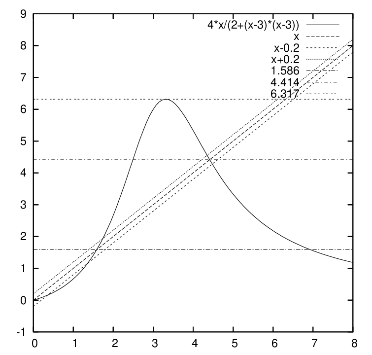
f(x):=\frac{4x}{2+(x-3)^{2}},\quad x>0.

(36)

The fixed points of $f$ in (36) are $c=3-\sqrt{2}\approx 1.586$ and $d=3+\sqrt{2}\approx 4.414$ . The maximum $f_{m}\approx 6.317$ is attained at $x_{m}=\sqrt{11}\approx 3.317$ . Also, $f(f_{m})\approx 1.943$ and the value of

d_{1}=\{x>d:f(x)=c\}\mbox{ ~is ~ }d_{1}=\frac{11}{3-\sqrt{2}}\approx 6.937.

Let us choose $a=1.8$ , $H=6.5$ , then $f(a)\approx 2.093$ , $f(H)\approx 1.825$ , then $F(a)=0.293$ , $F(H)\approx-4,675$ . We consider $l=0.2<0.293$ , for illustration of (36) see Fig. 2.

Furthermore, $b\approx 0.907$ , and $F(b)\approx-0.3384$ . For any $l<0.293$ , there is a domain $(0,v_{l})$ , starting with which we have low density behavior, and $(u_{l},H)$ which eventually leads a.s. to $(a,H)$ . Let us take $l=0.2$ , then $u_{l}\approx 1.74$ , $v_{l}\approx 0.361$ .

For (1) with $f$ as in (36), $l=0.2$ and $x_{0}\in[0,v_{l})=[0,0.36)$ we have low density behavior (Fig. 3, left), for $x_{0}\in(u_{l},H]=(1.74,6.5]$ we have persistence (Fig. 3, right). If $x_{0}\in(v_{l},u_{l})\approx(0.361,1.74)$ , then solutions can either sustain or have eventually low density (Fig. 3, middle). All numerical runs correspond to the case when $\chi$ has a uniform distribution on $[-1,1]$ .

Let us illustrate the dependency of the probability of the solution to sustain on the initial point $x_{0}\in(u_{l},v_{l})$ . Fig. 4 presents 10 random runs starting with $x_{0}=1.4,1.5,1.6,1.7$ (Fig. 4, from left to right).

For comparison, let us present several simulations for smaller $l=0.05$ , see Fig. 5.

Example 6.

Consider (1) with

f(x):=\frac{4x^{2}}{2+x}e^{2(1-x)},\quad x>0.

(37)

The fixed points are $c\approx 0.0833$ and $d\approx 1.2037$ , the maximum $f_{m}\approx 1.3688$ is attained at $\approx 0.8508$ . The minimum of $F(x)$ on $[0,c]$ is attained at $b\approx 0.0392$ and equals $F(b)\approx-0.0186$ .

Take $a=0.2$ , $H=1.8>f_{m}$ , $f(a)\approx 0.3602$ , $F(a)\approx 0.16$ , $f(H)\approx 0.6886>f(a)$ , $-F(H)\approx 1.111$ ; we can choose $l<0.16$ . If $l\in(-F(b),0.16)$ , or $l\in(0.0186,0.16)$ , we have persistence for any initial condition. All numerical runs are for the case when $\chi$ is uniformly distributed on $[-1,1]$ . We observe that for $l>-F(b)$ , say, $l=0.04$ , we have eventual persistence even for small $x_{0}=0.01$ (Fig. 6, left) while observe Allee effect for smaller $l=0.01<-F(b)$ and the same initial value (Fig. 6, right). This example illustrates the possibility to alleviate the Allee effect with large enough random noise. Fig. 6 (left) also illustrates the multi-step lifts to get into the persistence area.

7. Discussion

Complicated and chaotic behavior of even simple discrete systems leads to high risk of extinction. However, frequenly observed persistence suggested that there are some mechanisms for this type of dynamics. In the present paper, we proposed two mechanisms for sustaining a positive expectation in populations experiencing the Allee effect:

(1)

By Lemma 4.1, in the presence of a stochastic perturbation, there is a positive eventual expectation for any solution, independently of initial conditions. This can be treated as persistence thanks to some sustained levels of occasional immigration. However, the lower solution bound is still zero, and even expected solution averages are rather small and matched to this immigration probability distribution.
(2)

The second mechanism is more important for sustainability of populations. It assumes that there is a substantial range of values, where extinction due to either Allee effect or its combination with overpopulation reaction is impossible. For example, under contest competition [7] with the remaining population levels sufficient to sustain, even for initial values in the Allee zone, large enough stochastic perturbations lead to persistence. Specifically, the amplitude should exceed the maximal population loss in the Allee area, and at the same time should not endanger the original sustainability area. The result can be viewed as follows: if there is the Allee effect and sustainable dynamics for a large interval of values, introduction of a potentially large enough stochastic perturbation can lead to persistence, for any initial conditions.

For smaller perturbation amplitudes, there are 3 types of initial values: attracted to low dynamics a.s., a.s. persistent and those which can demonstrate each type of dynamics with a positive probability. As illustrated in Section 6, all three types of dynamics are possible.

In this paper we consider only bounded stochastic perturbations. The assumption of boundedness along with the properties of the function $f$ allows to construct a ”trap”, the interval $[a,H]$ , into which any solution eventually gets and stays there.

Assume for a moment that in equation (1) instead of bounded we have normally distributed $\chi_{n}$ . Applying the approach of the proof of Theorem 3.3 for bounded stochastic perturbations, we can show that for any initial value $x_{0}>0$ , a solution $x_{n}$ eventually gets into the interval $(a,H)$ , a.s. However, if $\chi_{n}$ can take any negative value with nonzero probability, applying the same method, we can show that there is a “sequence” of negative noises with an absolute value exceeding $H$ pushing the solution out of the interval $(a,H)$ , a.s. Thus, a.s., for any $n_{1}\in{\mathbb{N}}$ , there is an $n\geq n_{1}$ such that $x_{n}=0$ . So the conclusions of Lemma 3.2, (ii), and Theorem 3.3 are no longer valid.

Note that from the population model’s point of view the assumption that the noise is bounded is hardly a limitation since in nature there are no unbounded noises. For a normal type of noise, considering its truncation can be a reasonable approach to the problem.

8. Acknowledgment

The research was partially supported by NSERC grants RGPIN/261351-2010 and RGPIN-2015-05976 and also by AIM SQuaRE program. The authors are grateful to the ananymous reviewer whose valuable comments contributed to the present form of the paper.

References

[1] W. C. Allee, Animal Aggregations, a Study in General Sociology, University of Chicago Press, Chicago, 1931.
[2] J. A. D. Appleby, G. Berkolaiko and A. Rodkina, On local stability for a nonlinear difference equation with a non-hyperbolic equilibrium and fading stochastic perturbations, J. Difference Equ. Appl. 14 (2008), 923-–951.
[3] J. A. D. Appleby, G. Berkolaiko and A. Rodkina, Non-exponential stability and decay rates in nonlinear stochastic difference equations with unbounded noise, Stochastics 81 (2009), 99–127.
[4] J. A. D. Appleby, X. Mao and A. Rodkina, A. On stochastic stabilization of difference equations, Dynamics of Continuous and Discrete System 15 (2006), 843–857.
[5] G. Berkolaiko and A. Rodkina, Almost sure convergence of solutions to nonhomogeneous stochastic difference equation, J. Difference Equ. Appl. 12 (2006), 535-–553.
[6] D. S. Boukal and L. Berec, Single-species models of the Allee effect: extinction boundaries, sex ratios and mate encounters, J. Theor. Biol. 218 (2002), 375–394.
[7] F. Brauer and C. Castillo-Chavez, Mathematical Models in Population Biology and Epidemiology, Springer-Verlag New York, 2001.
[8] E. Braverman, Random perturbations of difference equations with Allee effect: switch of stability properties, Proceedings of the Workshop Future Directions in Difference Equations, 51–-60, Colecc. Congr., 69, Univ. Vigo, Serv. Publ., Vigo, 2011.
[9] E. Braverman and J. J. Haroutunian, Chaotic and stable perturbed maps: 2-cycles and spatial models, Chaos 20 (2010).
[10] E. Braverman and A. Rodkina, Stabilization of two-cycles of difference equations with stochastic perturbations, J. Difference Equ. Appl. 19 (2013), 1192–1212.
[11] E. Braverman and A. Rodkina, Difference equations of Ricker and logistic types under bounded stochastic perturbations with positive mean, Comput. Math. Appl. 66 (2013), 2281–2294.
[12] M. A. Burgman, S. Ferson and H. R. Akćakaya, Risk Assessment in Conservation Biology, London: Chapman & Hall, 1993.
[13] S. N. Cohen and R. J. Elliott, Backward stochastic difference equations and nearly time-consistent nonlinear expectations, SIAM J. Control Optim. 49 (2011), 125-–139.
[14] N. Dokuchaev and A. Rodkina, Instability and stability of solutions of systems of nonlinear stochastic difference equations with diagonal noise, J. Difference Equ. Appl. 14 (2014), 744–764.
[15] F. C. Hoppensteadt, Mathematical Methods of Population Biology, Cambridge, MA: Cambridge University Press, 1982.
[16] J. Jacobs, Cooperation, optimal density and low density thresholds: yet another modification of the logistic model, Oecologia 64 (1984), 389-395.
[17] C. Kelly and A. Rodkina, Constrained stability and instability of polynomial difference equations with state-dependent noise, Discrete Contin. Dyn. Syst. Ser. B 11 (2009), 913–933.
[18] V. Kolmanovskii and L. Shaikhet, Some conditions for boundedness of solutions of difference Volterra equations, Appl. Math. Lett. 16 (2003), 857–862.
[19] A. Rodkina and M. Basin, On delay-dependent stability for vector nonlinear stochastic delay-difference equations with Volterra diffusion term, Syst. Control Lett. 56 (2007), 423–430.
[20] S. J. Schreiber, Allee effect, extinctions, and chaotic transients in simple population models, Theor. Popul. Biol. 64 (2003), 201–209.
[21] S. J. Schreiber, Persistence for stochastic difference equations: a mini-review, J. Difference Equ. Appl. 18 (2012), 1381-–1403.
[22] L. Shaikhet, Lyapunov Functionals and Stability of Stochastic Difference Equations, Springer, London, 2011.
[23] A. N. Shiryaev, Probability (2nd edition), Springer, Berlin, 1996.

Stochastic difference equations with the Allee effectThanks: E. Braverman is a corresponding author, e-mail maelena@ucalgary.ca.

Abstract.

Key words and phrases:

1991 Mathematics Subject Classification

1. Introduction

2. Preliminaries

Assumption 1.

Assumption 2.

Assumption 3.

3. Unconditional Persistence and Low-Density Behavior

Lemma 3.1.

Proof.

Remark 1.

Lemma 3.2.

Proof.

Remark 2.

Theorem 3.3.

Proof.

Corollary 1.

4. Dynamics Depending on Perturbations (the case l<b−f⁡(b)l<b-f(b))

Lemma 4.1.

Proof.

4.1. A.s. persistence and a.s. low density areas

Theorem 4.2.

Proof.

4.2. Mixed behavior

Remark 3.

Example 1.

Lemma 4.3.

Proof.

Remark 4.

Remark 5.

Corollary 2.

Proof.

Lemma 4.4.

Remark 6.

Example 2.

Theorem 4.5.

Lemma 4.6.

Proof.

4.3. FF is increasing on (b,a)(b,a)

Corollary 3.

Theorem 4.7.

Proof.

Corollary 4.

Proof.

5. Multistability

Assumption 4.

Lemma 5.1.

Proof.

Example 3.

Example 4.

6. Numerical Examples

Example 5.

Example 6.

7. Discussion

8. Acknowledgment

References

4. Dynamics Depending on Perturbations (the case $l<b-f(b)$ )

4.3. $F$ is increasing on $(b,a)$