Mocking the Weak Lensing universe: the LensTools python computing package
Abstract
We present a newly developed software package which implements a wide range of routines frequently used in Weak Gravitational Lensing (WL). With the continuously increasing size of the WL scientific community we feel that easy to use Application Program Interfaces (APIs) for common calculations are a necessity to ensure efficiency and coordination across different working groups. Coupled with existing open source codes, such as CAMB[1] and Gadget2[2], LensTools brings together a cosmic shear simulation pipeline which, complemented with a variety of WL feature measurement tools and parameter sampling routines, provides easy access to the numerics for theoretical studies of WL as well as for experiment forecasts. Being implemented in python[3], LensTools takes full advantage of a range of state–of–the art techniques developed by the large and growing open–source software community [4, 5, 6, 7, 8]. We made the LensTools code available on the Python Package Index and published its documentation on http://lenstools.readthedocs.io
Keywords:
Weak Gravitational Lensing , SimulationsPACS
98.80.-k , 95.36.+x , 95.30.Sf , 98.62.Sb1 Introduction
Cosmology is entering a data driven era. After the Cosmic Microwave Background (CMB) [9, 10] provided strong experimental evidences of cosmological theories, a variety of different probes have been proposed to unveil the secret of the cosmos. Weak Gravitational Lensing uses the correlation between image distortions of background sources by Large Scale Structure (LSS) to infer cosmological parameter values [11]. Because WL probes are sensitive to late universe physics, where the density fluctuations are in the non–linear regime, quadratic features such as two–point correlation functions might miss some of the cosmological information. In the theoretical study of more complicated WL features (see for example [12, 13, 14, 15] for a non comprehensive list) simulation pipelines play a vital role, as in general these features cannot be predicted analytically from cosmological parameters. In this work we present a flexible, customizable and easy to deploy WL simulation pipeline that bridges the gap between simulations of shear fields, feature measurement from simulated images and cosmological parameter estimation. The paper is organized as follows: first we give an overview of the shear field simulation routines and present their runtime and memory usage benchmarks. We then outline the LensTools image analysis capabilities as well as the parameter estimation routines. We finally present a summary of our work and outline our conclusions. We complement our work with some illustrative coding examples that show how to operationally use LensTools for some of the former tasks.
2 Shear simulations
2.1 Formalism
In this paragraph we give an overview of the LensTools shear field simulation pipeline. This consists in a series of routines that, starting from a CDM cosmological model specified by the cosmological parameters
| (1) |
produces random realizations of shear fields in cosmology . Here is the angle on sky as seen from the observer. Given a background source (such as a galaxy) at redshift , the dark matter density fluctuations between the observer and the source will cause its apparent shape to be distorted due to the gravitational lensing effect, as predicted by General Relativity [16]. The apparent source ellipticity, assuming the unperturbed shape is a circle, can be estimated in terms of the cosmic shear defined in equation (12). Non circular shapes can be modeled with redshift–dependent shape noise terms [16], the treatment of which goes beyond the scope of this paper. The multi–lens–plane algorithm [17, 18, 19, 20] is a popular technique to compute light ray deflections across the path and hence to compute the apparent source shape distortion. The mass distribution between the source and the observer is approximated as a finite set of two dimensional lenses perpendicular to the line of sight, of thickness and a surface density given by
| (2) |
where is the lens comoving distance and the scale factor. A light ray crossing a lens at redshift at a transverse position will be deflected by a small angle which can be shown to be the gradient of the 2D gravitational potential (see again [17])
| (3) |
| (4) |
| (5) |
where we indicated as the gradient of the deflection, which will be called distortion tensor throughout the rest of the paper. An example of a lens plane computed with the LensTools pipeline according to equations (2),(3) is shown in Figure 1.


The trajectory of a light ray follows the geodesic equation
| (6) |
which can be translated into a second order differential equation for the light ray angular position as seen from the observer. Following [17], the trajectory of each light ray originating at can be calculated solving numerically a discretized version of (6), assuming a finite number of lenses placed at redshifts :
| (7) |
| (8) |
| (9) |
| (10) |
where is the Jacobian matrix of the trajectory with respect to the initial light ray position , . The factors depend on the geometry of the lens system
| (11) |
where we use the subscript to indicate the redshift of the –th lens for notational simplicity. After tracing the evolution of from the observer to the source at , we are able to evaluate the cosmic shear and convergence at looking at the components of
| (12) |
The solution of equation (6) via the multi–lens–plane algorithm yields a single realization of the WL fields . Multiple random realizations of these fields can be obtained by altering the lens system before ray–tracing using the randomization technique described in [21].
The iterative solution of equations (7)–(10) requires knowledge of the density fluctuation , from which the lens surface density and gravitational potential can be inferred through equations (2),(3). can be calculated running numerical simulations, such as –body simulations [2, 22] or hydrodynamical simulations [23]. In this paragraph we focus mainly on –body simulations, in which the matter distribution in the universe is approximated as a set of particles of mass , which move in their self–generated gravitational field. For this purpose we use the publicly available code Gadget2[2], although alternatives can be adopted (see [22] for example). Once the –body simulations are run, LensTools provides a python implementation of the multi–lens–plane algorithm [17] described above, which takes care of projecting the density fluctuation on two dimensional lenses as in (2), solving the Poisson equation as in (3), and computing the light ray deflections as in (7)–(10). An overview of the pipeline operations, from the cosmological parameter specifications to the final shear map products, is outlined in Figure 2. We make the claim that the way the LensTools code is organized makes it portable between different research groups that rely on different choices, rather than Gadget2, for running –body simulations. The transition between snapshots and lens planes is handled by instances of the NbodySnapshot class, which implements the algorithms based on equations (3). NbodySnapshot can be sub–classed to implement the necessary input routines from the –body snapshots. LensTools comes with one of such possibilities, the Gadget2Snapshot class, that handles input from snapshots in the Gadget2 binary format. Other subclass types that allow input from other formats can be coded by the user with minimal effort.

2.2 Pipeline code structure
In this paragraph we describe how the LensTools pipeline code is organized. The simulation products are placed in a directory tree structure designed for easy resource access. The directory tree is mirrored in two locations, a so called Home location, which holds all the book–keeping information such as small data files (such as CAMB matter power spectra) and configuration files, and a Storage location which holds the simulation products (Gadget2 snapshots, lens planes and finished shear maps). The reason for this is that while the Home location does not require much disk space, the Storage location can reach disk sizes of several Terabytes. We found it convenient to keep the two locations separated to simplify sharing data among machines in a cluster, and help with portability issues among different clusters. A batch of simulations is handled by a single instance of a SimulationBatch object (which holds both the Home and Storage parts). The first level in the tree corresponds to a choice of values for cosmological parameters : each node on this level of the tree is an instance of the SimulationModel class. The second level in the tree specifies the size and resolution of the –body box, namely the box size and the number of particles : each node on the second level corresponds to a SimulationCollection object. Inside a simulation collection, we are free to choose different random realizations of the initial conditions, which will then be evolved in time by the –body code. Each such realization lives on a node which is one level deeper in the tree, and is encoded in a SimulationIC object. The deepest level in the tree contains the two dimensional slices of the –body simulation boxes. Each node on this level is an instance of the SimulationPlanes class. Once the lens planes are generated, the ray–tracing operations can be performed. In principle we can use lens planes that live under the same SimulationCollection, but belong to different SimulationIC nodes, to produce either single redshift shear images (each ensemble of images lives in a SimulationMaps object) or shear catalogs of sources, in the form of a table in which each of the rows is a tuple . Each ensemble of catalogs corresponds to an instance of the SimulationCatalog class. Note that, because they combine lens planes with different initial random seed (see [21]), both SimulationMaps and SimulationCatalog nodes live on the same level of the directory tree, one level below SimulationCollection. An example on how to create a python script to lay down such a directory tree is available in IPython notebook format11 1 http://nbviewer.jupyter.org/github/apetri/LensTools/blob/master/notebooks/dirtree.ipynb. A comprehensive guide on how to deploy the LensTools simulation pipeline on a computer cluster can be found in the code documentation [24].
2.3 Performance
We summarize the runtime and memory usage benchmarks of the LensTools shear simulation pipeline. The tests were run on the XSEDE Stampede computer cluster22 2 https://portal.xsede.org/tacc-stampede. Table 1 shows a summary of the ray–tracing operations performed by LensTools , indicating the complexity and runtime of each operation for a selected test case. At the lens plane generation stage we can clearly see that the two bottlenecks in the flow are the read operations from –body snapshot files and the Poisson equation solving via FFT. The number of tasks used to read in a single snapshot can be optimized if the parallel input performance is ideal (i.e independent on ), as is an optimal value of that minimizes the combined input, gridding and MPI communication operations, which have a combined complexity
| (13) |
The optimal depends on the number of particles and the lens plane resolution (in pixels) . In principle this bottleneck can be removed if the capability of generating lens planes is embedded into the –body code, which could avoid saving the intermediate 3D snapshots to disk. LensTools allows such a possibility by creating a channel of communication between Gadget2 and the plane application using named pipes. For this option to be viable, Gadget2 and the plane computation must run on the same node.
The Poisson solver has a complexity of which is dominated by FFT performance. Although we make use of the numpy FFT pack [4] to perform such operations, other alternatives are also possible (such as FFTW [25]). The LensTools code modularity makes it very easy to switch between different implementations of the FFT algorithm, both coming from external libraries or coded up by the user. The bottleneck of the ray–tracing operations consists in the calculations of the ray deflections in equation (8) and the distortion tensor products (10). Although the complexity of these operations is already optimal, improvements on the runtime can be made by using specialized libraries to handle matrix products. numpy can link to the most up–to–date version of specialized libraries such as LAPACK [26] and Intel MKL [27]. Some versions of numpy even support automatic offload of linear algebra operations to Intel XEON Phi co–processors [28].
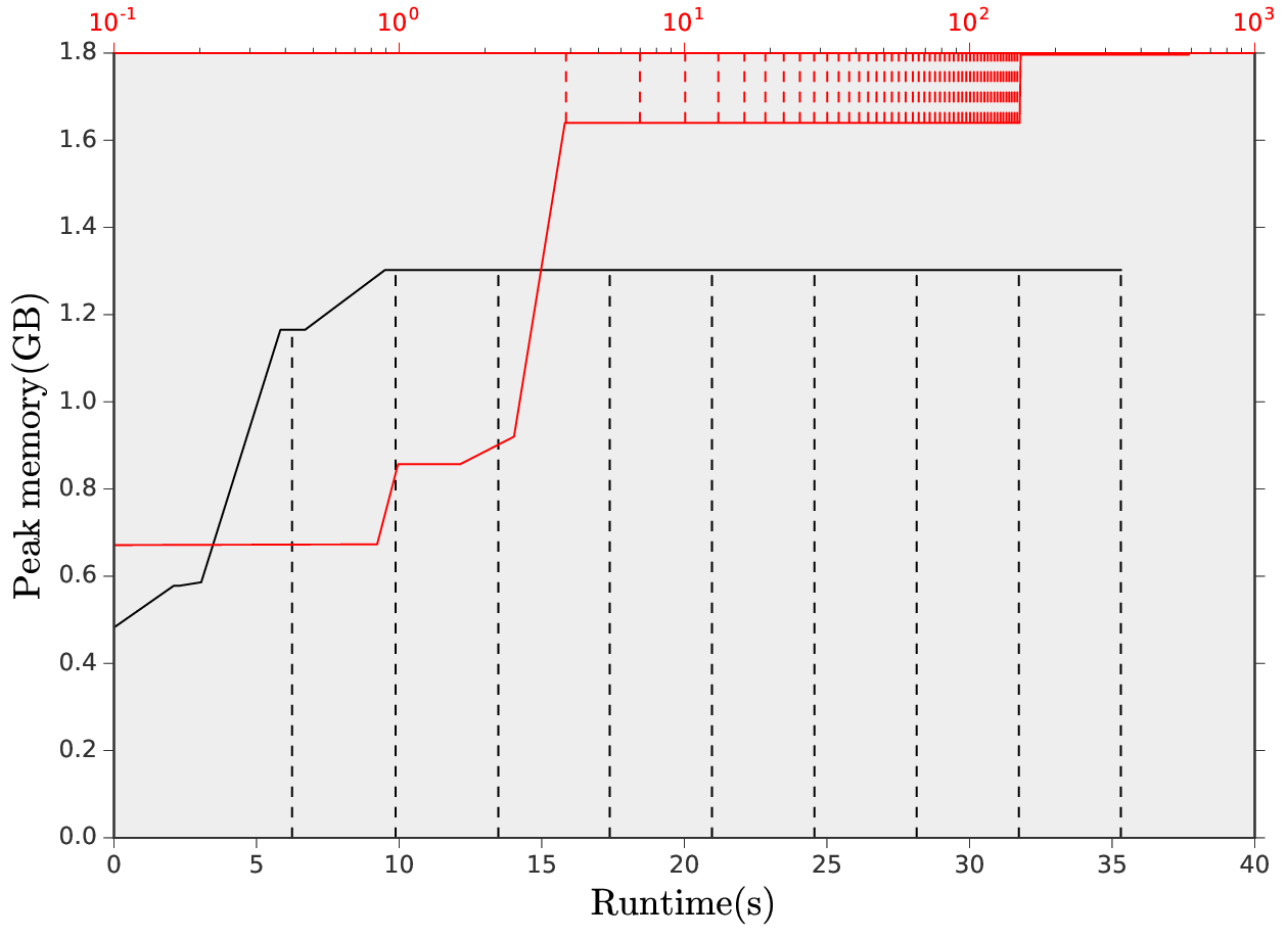
We tracked the memory usage of the lens plane and ray–tracing operations. This is an important step, since python has some subtleties when dealing with large memory applications. Memory allocated by a python process cannot be released manually as in C, but is managed by the built–in garbage collector instead. Figure 3 shows the peak memory usage during the lens plane generation and ray–tracing operations. We can see that, for the test case outlined in Table 1, memory consumption stabilizes around 1.3 GB per task for the lens planes and 1.8 GB per task during the ray–tracing. These considerations make the LensTools pipeline suitable for deployment on computer clusters with 2 GB memory per core, such as the one we used. These numbers refer to the test case described in Table 1. Producing higher resolution lens planes and WL maps will in general require more memory. A rough estimate for the memory scaling with resolution can be made noting that the dominant contribution to the memory usage for the lens planes comes from the input from the –body simulations and should hence scale with the number of particles . For the ray–tracing, on the other hand, the dominant contribution to the memory usage comes from the lenses and should hence scale as the lens pixel resolution , also because the resolution of the WL maps needs to be smaller than .
| Step | Complexity | Test case | Runtime |
| Lens generation | |||
| Snapshot input | , | 2.10 s | |
| Gridding | , | 0.20 s | |
| MPI Communication | , | 0.76 s | |
| Poisson solver (FFT) | 2.78 s | ||
| Lens output | 0.04 s | ||
| Ray tracing | |||
| Lens input | 0.32 s | ||
| Random lens shift | 0.15 s | ||
| Deflection calculation | 1.54 s | ||
| Shear tensor product | 1.29 s | ||
3 Image analysis
In this section we describe some useful routines that LensTools provides for analyzing simulated convergence and shear fields. The ConvergenceMap and ShearMap classes implement several operations that can be performed on two dimensional images (for a complete list look at the LensTools documentation [24]). Both classes allow flexible I/O formats from files through the load method (the FITS format [31] is a popular choice, but not the only one possible; user custom format can be easily dealt within LensTools ). Efficient routines are available for smoothing the maps with Gaussian kernels (optimal smoothing complexity–wise can be performed via FFT for kernel sizes bigger than pixel, otherwise real–space techniques are preferrable. LensTools allows for both possibilities.), measuring the pixel PDF, counting the local maxima and measuring their position, measuring topological descriptors such as Minkowski Functionals [32]. An example of such operations is shown in Figure 4.


In addition to real space statistics such as the ones outlined before, LensTools provides access to quadratic Fourier statistics such as power spectra. The convergence angular power spectrum is defined as
| (14) |
where we indicate the Fourier transform of as . The shear field can be decomposed into its and components according to
| (15) |
Because of the nature of the density perturbations that cause background source lensing, the component dominates in the weak lensing limit, because and . The shear –mode is the convergence (in Fourier space), hence . Figure 5 shows the shear and modes power spectra measured from one realization of the shear field.

4 Cosmology constraints
4.1 Formalism
In this section we outline the basic routines that LensTools provides for constraining cosmology. Let be the parameters to constrain (for example ) and let be a WL feature that contains information on . An example of can be the power spectrum defined in (14). Given a feature measurement , we are interested in calculating the likelihood of the parameters, given the measurement. Using the Bayes theorem we can express the parameter likelihood as
| (16) |
where is the prior on the parameters, is a –independent normalization constant and is the feature likelihood. A popular choice for the feature likelihood is a normal distribution with mean and covariance , with
| (17) |
LensTools provides efficient routines for computing (17) at arbitrary points in parameter space. We argue that efficient evaluation of is not only useful when data likelihoods are Gaussian, but also gives access to more advanced likelihood sampling methods such as Approximate Bayesian Computation [33]. Running the simulation pipeline described in § 2 for a variety of cosmological models , , gives access to a discrete set of features evaluated at . We are able to evaluate equation (17) at an arbitrary point in parameter space using a Radial Basis Function (RBF) interpolation scheme
| (18) |
where is an isotropic smoothing kernel of scale 33 3 For the examples shown in this work we chose a multiquadric kernel with chosen as the mean distance between the simulated points and the weights can be determined from the known simulated features with a matrix inversion
| (19) |
Once the weights are determined from the simulated features, equation (18) allows for a fast vectorized evaluation of the parameter likelihood from equations (16),(17) once an assumption for the (–independent) covariance matrix is made. A possible choice is estimating the covariance from the shear simulations themselves 44 4 In the case in which the covariance matrix is estimated from simulations, the estimator for its inverse is biased [34]. LensTools sampling routines use the unbiased estimator where is the number of realizations used to estimate the feature covariance. Having access to an efficient routine for computing the parameter likelihood allow access to a variety of parameter sampling techniques. In this section we give examples of three different parameter sampling techniques supported in LensTools :
- 1.
Likelihood Grid Evaluation: if the dimensionality of the parameter space is not too big, the parameter likelihood in equation (16) can be evaluated on a regularly spaced grid of points. Since each point can be treated independently, this procedure is easily parallelizable. LensTools provides a parallel implementation of the likelihood grid evaluation based on the MPI protocol [30]. Access to the values of the likelihood on a regularly spaced grid makes the determination of confidence intervals straightforward. Such an approach has been used before in the literature [35, 36].
- 2.
MCMC sampling of the parameter space: the efficient LensTools likelihood evaluation routines are specifically designed to be compatible with widely used python packages such as emcee [8] and pymc [37] that specialize in generating parameter samples with the Markov Chain Monte Carlo (MCMC) technique [38]. emcee supports parallel MCMC sampling via mpi4py.
- 3.
Fisher Matrix approximation: for the sake of simplicity, sometimes it is convenient to approximate the parameter likelihood as a Gaussian centered around its maximum. If we have a reasonable guess for the likelihood peak location (in the case where the likelihood is single–modal), the parameter covariance matrix can be approximated as
(20) The partial derivatives of the likelihood with respect to the parameters are easy to evaluate with finite differences.
4.2 Code structure
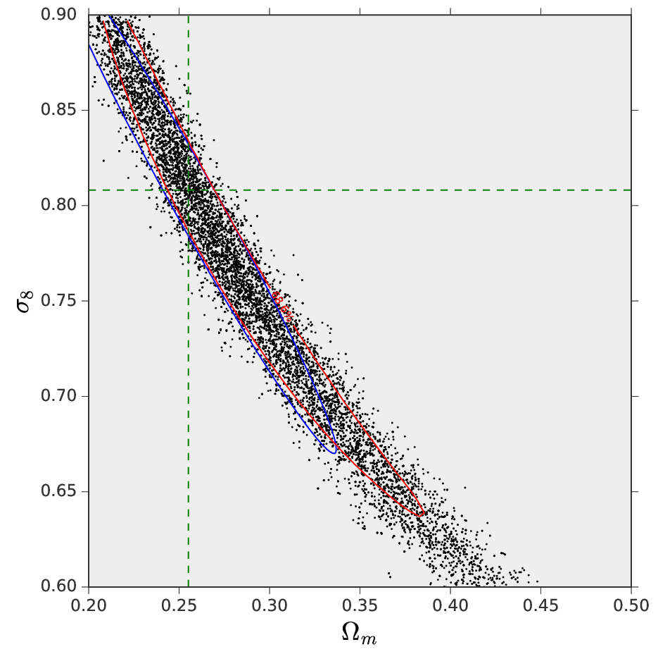
We give a brief overview of the LensTools object types that handle parameter constraints operations. Feature emulators in LensTools are row–oriented data structures, in which each of the rows contains a tuple of cosmological (and/or nuisance) parameters and the simulated feature at . The base class that handles row–oriented data in LensTools is the Ensemble class. Ensemble inherits from pandas.DataFrame [5] and provides additional routines for feature measurement from simulations (both serial and parallel in the number of maps with mpi4py [29]), Principal Component Analysis, statistics bootstrapping. As a sub–class of pandas.DataFrame, Ensemble supports I/O and queries from local and remote SQL databases. Parameter space sampling operations in LensTools are handled by instances of the Emulator class, which inherits from Ensemble and provides access to vectorized RBF feature interpolation between parameters (which can be used to build emulators), evaluation, and the parameter sampling techniques outlined above. Examples of parameter sampling routines are shown in Figure 6.
5 Conclusion
In this work we presented the LensTools computing package, which is a collection of tools targeted to theoretical studies of WL. The package includes a WL shear simulation pipeline and is complemented with a variety of image analysis tools and parameter sampling routines. The simulation pipeline combines different existing codes to simulate cosmological volumes (CAMB,Gadget2) and provides a python implementation of the multi–lens–plane algorithm. LensTools is flexible in terms of snapshot file formats, making the use of different –body simulation codes (see [22] for example) possible with minimal additional efforts. This makes LensTools portable between different research groups in the WL community. LensTools makes use of the numpy array as its primary data structure for numerical calculations, making it very convenient to combine with popular algorithmic packages for data selection (pandas [5]), astronomical tools (astropy [6]), MCMC sampling (pymc [37], emcee [8]), advanced statistical analysis and machine learning (scikit-learn [7]). Because of these reasons, we believe that LensTools will become a valuable asset to the WL community, in particular to groups that already have experience with –body simulations and want to study Weak Lensing.
Acknowledgements
We thank Zoltàn Haiman, Jia Liu, Jose M. Zorrilla and Morgan May for invaluable support and useful discussions. The simulations in this work were performed at the NSF Extreme Science and Engineering Discovery Environment (XSEDE), supported by grant number ACI-1053575, at the Yeti computing cluster at Columbia University, and at the New York Center for Computational Sciences, a cooperative effort between Brookhaven National Laboratory and Stony Brook University, supported in part by the State of New York. This work was supported in part by the U.S. Department of Energy under Contract Nos. DE-AC02-98CH10886 and DESC0012704, and by the NSF Grant No. AST-1210877 (to Z.H.) and by the Research Opportunities and Approaches to Data Science (ROADS) program at the Institute for Data Sciences and Engineering at Columbia University.
References
- [1] A. Lewis, A. Challinor, A. Lasenby, Efficient computation of CMB anisotropies in closed FRW models, Astrophys. J. 538 (2000) 473–476. arXiv:astro-ph/9911177.
- [2] V. Springel, The cosmological simulation code GADGET-2, MNRAS364 (2005) 1105–1134. arXiv:astro-ph/0505010, doi:10.1111/j.1365-2966.2005.09655.x.
- [3] G. Rossum, Python reference manual, Tech. rep., Amsterdam, The Netherlands, The Netherlands (1995).
- [4]
E. Jones, T. Oliphant, P. Peterson, et al.,
SciPy: Open source scientific tools for
Python, [Online; accessed 2015-11-13] (2001–).
URL http://www.scipy.org/ - [5] W. McKinney, Data structures for statistical computing in python, in: S. van der Walt, J. Millman (Eds.), Proceedings of the 9th Python in Science Conference, 2010, pp. 51 – 56.
- [6] Astropy Collaboration, T. P. Robitaille, E. J. Tollerud, P. Greenfield, M. Droettboom, E. Bray, T. Aldcroft, M. Davis, A. Ginsburg, A. M. Price-Whelan, W. E. Kerzendorf, A. Conley, N. Crighton, K. Barbary, D. Muna, H. Ferguson, F. Grollier, M. M. Parikh, P. H. Nair, H. M. Unther, C. Deil, J. Woillez, S. Conseil, R. Kramer, J. E. H. Turner, L. Singer, R. Fox, B. A. Weaver, V. Zabalza, Z. I. Edwards, K. Azalee Bostroem, D. J. Burke, A. R. Casey, S. M. Crawford, N. Dencheva, J. Ely, T. Jenness, K. Labrie, P. L. Lim, F. Pierfederici, A. Pontzen, A. Ptak, B. Refsdal, M. Servillat, O. Streicher, Astropy: A community Python package for astronomy, A&A558 (2013) A33. arXiv:1307.6212, doi:10.1051/0004-6361/201322068.
- [7] F. Pedregosa, G. Varoquaux, A. Gramfort, V. Michel, B. Thirion, O. Grisel, M. Blondel, P. Prettenhofer, R. Weiss, V. Dubourg, J. Vanderplas, A. Passos, D. Cournapeau, M. Brucher, M. Perrot, E. Duchesnay, Scikit-learn: Machine learning in Python, Journal of Machine Learning Research 12 (2011) 2825–2830.
- [8] D. Foreman-Mackey, D. W. Hogg, D. Lang, J. Goodman, emcee: The mcmc hammer, PASP 125 (2013) 306–312. arXiv:1202.3665, doi:10.1086/670067.
- [9] C. L. Bennett, D. Larson, J. L. Weiland, N. Jarosik, G. Hinshaw, N. Odegard, K. M. Smith, R. S. Hill, B. Gold, M. Halpern, E. Komatsu, M. R. Nolta, L. Page, D. N. Spergel, E. Wollack, J. Dunkley, A. Kogut, M. Limon, S. S. Meyer, G. S. Tucker, E. L. Wright, Nine-year Wilkinson Microwave Anisotropy Probe (WMAP) Observations: Final Maps and Results, ApJS208 (2013) 20. arXiv:1212.5225, doi:10.1088/0067-0049/208/2/20.
- [10] Planck Collaboration, P. A. R. Ade, N. Aghanim, C. Armitage-Caplan, M. Arnaud, M. Ashdown, F. Atrio-Barandela, J. Aumont, C. Baccigalupi, A. J. Banday, et al., Planck 2013 results. XVI. Cosmological parameters, A&A571 (2014) A16. arXiv:1303.5076, doi:10.1051/0004-6361/201321591.
- [11] M. Bartelmann, P. Schneider, Weak gravitational lensing, Phys. Rep.340 (2001) 291–472. arXiv:astro-ph/9912508, doi:10.1016/S0370-1573(00)00082-X.
- [12] M. Takada, B. Jain, Three-point correlations in weak lensing surveys: model predictions and applications, MNRAS344 (2003) 857–886. arXiv:astro-ph/0304034, doi:10.1046/j.1365-8711.2003.06868.x.
- [13] M. Takada, B. Jain, Cosmological parameters from lensing power spectrum and bispectrum tomography, MNRAS348 (2004) 897–915. arXiv:astro-ph/0310125, doi:10.1111/j.1365-2966.2004.07410.x.
- [14] F. Bernardeau, L. van Waerbeke, Y. Mellier, Weak lensing statistics as a probe of OMEGA and power spectrum., A&A322 (1997) 1–18. arXiv:astro-ph/9609122.
- [15] B. Jain, L. Van Waerbeke, Statistics of Dark Matter Halos from Gravitational Lensing, ApJ530 (2000) L1–L4. arXiv:astro-ph/9910459, doi:10.1086/312480.
- [16] P. Schneider, Weak Gravitational Lensing, ArXiv Astrophysics e-printsarXiv:astro-ph/0509252.
- [17] S. Hilbert, J. Hartlap, S. D. M. White, P. Schneider, Ray-tracing through the Millennium Simulation: Born corrections and lens-lens coupling in cosmic shear and galaxy-galaxy lensing, A&A499 (2009) 31–43. arXiv:0809.5035, doi:10.1051/0004-6361/200811054.
- [18] T. Hamana, Y. Mellier, Numerical study of the statistical properties of the lensing excursion angles, MNRAS327 (2001) 169–176. arXiv:astro-ph/0101333, doi:10.1046/j.1365-8711.2001.04685.x.
- [19] M. Sato, T. Hamana, R. Takahashi, M. Takada, N. Yoshida, T. Matsubara, N. Sugiyama, Simulations of Wide-Field Weak Lensing Surveys. I. Basic Statistics and Non-Gaussian Effects, ApJ701 (2009) 945–954. arXiv:0906.2237, doi:10.1088/0004-637X/701/2/945.
- [20] B. M. Schäfer, L. Heisenberg, A. F. Kalovidouris, D. J. Bacon, On the validity of the Born approximation for weak cosmic flexions, MNRAS420 (2012) 455–467. arXiv:1101.4769, doi:10.1111/j.1365-2966.2011.20051.x.
- [21] A. Petri, Z. Haiman, M. May, Sample variance in weak lensing: how many simulations are required?, ArXiv e-printsarXiv:1601.06792.
- [22] S. Habib, A. Pope, H. Finkel, N. Frontiere, K. Heitmann, D. Daniel, P. Fasel, V. Morozov, G. Zagaris, T. Peterka, V. Vishwanath, Z. Lukić, S. Sehrish, W.-k. Liao, HACC: Simulating sky surveys on state-of-the-art supercomputing architectures 42 (2016) 49–65. arXiv:1410.2805, doi:10.1016/j.newast.2015.06.003.
- [23]
A. Dubey, K. Antypas, A. C. Calder, C. Daley, B. Fryxell, J. B. Gallagher,
D. Q. Lamb, D. Lee, K. Olson, L. B. Reid, P. Rich, P. M. Ricker, K. M. Riley,
R. Rosner, A. Siegel, N. T. Taylor, K. Weide, F. X. Timmes, N. Vladimirova,
J. Zuhone, Evolution of
flash, a multi-physics scientific simulation code for high-performance
computing, Int. J. High Perform. Comput. Appl. 28 (2) (2014) 225–237.
doi:10.1177/1094342013505656.
URL http://dx.doi.org/10.1177/1094342013505656 - [24] The lenstools documentation, http://lenstools.readthedocs.io.
- [25] M. Frigo, S. G. Johnson, The design and implementation of FFTW3, Proceedings of the IEEE 93 (2) (2005) 216–231, special issue on “Program Generation, Optimization, and Platform Adaptation”.
- [26] E. Anderson, Z. Bai, C. Bischof, S. Blackford, J. Demmel, J. Dongarra, J. Du Croz, A. Greenbaum, S. Hammarling, A. McKenney, D. Sorensen, LAPACK Users’ Guide, 3rd Edition, Society for Industrial and Applied Mathematics, Philadelphia, PA, 1999.
- [27] Intel Math Kernel Library. Reference Manual, Intel Corporation, 2009, santa Clara, USA. ISBN 630813-054US.
- [28] R. Rahman, Intel Xeon Phi Coprocessor Architecture and Tools: The Guide for Application Developers, 1st Edition, Apress, Berkely, CA, USA, 2013.
- [29]
L. Dalcín, R. Paz, M. Storti,
{MPI}
for python, Journal of Parallel and Distributed Computing 65 (9) (2005) 1108
– 1115.
doi:http://dx.doi.org/10.1016/j.jpdc.2005.03.010.
URL http://www.sciencedirect.com/science/article/pii/S0743731505000560 - [30] M. P. Forum, Mpi: A message-passing interface standard, Tech. rep., Knoxville, TN, USA (1994).
- [31] W. Pence, CFITSIO, v2.0: A New Full-Featured Data Interface, in: D. M. Mehringer, R. L. Plante, D. A. Roberts (Eds.), Astronomical Data Analysis Software and Systems VIII, Vol. 172 of Astronomical Society of the Pacific Conference Series, 1999, p. 487.
- [32] T. Matsubara, Analytic Minkowski functionals of the cosmic microwave background: Second-order non-Gaussianity with bispectrum and trispectrum, Phys. Rev. D81 (8) (2010) 083505. arXiv:1001.2321, doi:10.1103/PhysRevD.81.083505.
- [33] E. E. O. Ishida, S. D. P. Vitenti, M. Penna-Lima, J. Cisewski, R. S. de Souza, A. M. M. Trindade, E. Cameron, V. C. Busti, COSMOABC: Likelihood-free inference via Population Monte Carlo Approximate Bayesian Computation, Astronomy and Computing 13 (2015) 1–11. arXiv:1504.06129, doi:10.1016/j.ascom.2015.09.001.
- [34] A. Taylor, B. Joachimi, T. Kitching, Putting the precision in precision cosmology: How accurate should your data covariance matrix be?, MNRAS432 (2013) 1928–1946. arXiv:1212.4359, doi:10.1093/mnras/stt270.
- [35] J. Liu, A. Petri, Z. Haiman, L. Hui, J. M. Kratochvil, M. May, Cosmology constraints from the weak lensing peak counts and the power spectrum in CFHTLenS data, Phys. Rev. D91 (6) (2015) 063507. arXiv:1412.0757, doi:10.1103/PhysRevD.91.063507.
- [36] A. Petri, J. Liu, Z. Haiman, M. May, L. Hui, J. M. Kratochvil, Emulating the CFHTLenS weak lensing data: Cosmological constraints from moments and Minkowski functionals, Phys. Rev. D91 (10) (2015) 103511. arXiv:1503.06214, doi:10.1103/PhysRevD.91.103511.
- [37] A. Patil, D. Huard, C. Fonnesbeck, Pymc: Bayesian stochastic modelling in python, Journal of Statistical Software 35 (1) (2010) 1–81.
- [38]
C. Andrieu, N. de Freitas, A. Doucet, M. I. Jordan,
An introduction to mcmc for
machine learning, Machine Learning 50 (1) 5–43.
doi:10.1023/A:1020281327116.
URL http://dx.doi.org/10.1023/A:1020281327116