A combined Lattice Boltzmann and Immersed Boundary approach for predicting the vascular transport of differently shaped particles
Abstract
Modelling the vascular transport and adhesion of man-made particles is crucial for optimizing their efficacy in the detection and treatment of diseases. Here, a Lattice Boltzmann and Immersed Boundary methods are combined together for predicting the near wall dynamics of particles with different shapes in a laminar flow. For the lattice Boltzmann modelling, a Gauss-Hermite projection is used to derive the lattice equation; wall boundary conditions are imposed through the Zou-He framework; and a moving least squares algorithm accurately reconstructs the forcing term accounting for the immersed boundary. First, the computational code is validated against two well-known test cases: the sedimentation of circular and elliptical cylinders in a quiescent fluid. A very good agreement is observed between the present results and those available in the literature. Then, the transport of circular, elliptical, rectangular, square and triangular particles is analyzed in a Couette flow, at Re=20. All particles drifted laterally across the stream lines reaching an equilibrium position, independently of the initial conditions. For this large Reynolds number, the particle shape has no significant effect on the final equilibrium position but it does affect the absolute value and periodicity of the angular velocity. Specifically, elongated particles show longer oscillation periods and, most interestingly, larger variations in angular velocity. The longest particles exhibit a zero angular velocity for almost the whole rotational period. Collectively, this data demonstrates that the proposed approach can be efficiently used for predicting complex particle dynamics in biologically relevant flows. This computational strategy could have significant impact in the field of computational nanomedicine for optimizing the specific delivery of therapeutic and imaging agents.
Keywords:
Particle transport , Lattice-Boltzmann , Immersed boundary , Neutrally buoyant particle , Shear flowIntroduction
The intravenous administration of nanoconstructs for the precise delivery of therapeutic and imaging agents has been demonstrated to have potential in the fight against deadly diseases, such as cancer and cardiovascular diseases [1, 2]. Nanoconstructs are man-made, biocompatible and biodegradable objects that transported by the blood flow can reach any location within the vascular network and release their therapeutic cargo thereof [3, 4, 5]. Over the last decade, nanoconstructs exhibiting different sizes, shapes, surface properties and, more recently, also mechanical stiffnesses have been presented [6, 7, 8, 9, 10]. The size can range from a few tens of nanometers to a few microns; the shape can be spherical, discoidal, cylindrical; the surface can exhibit a positive, negative or neutral electrostatic charge and can be decorated with a variety of moieties for specific cell recognition; and the stiffness can vary from that of cells to metals. Size, shape, surface and stiffness have been shown by the authors and others to significantly affect the vascular and extravascular behaviour of systemically injected nanoconstructs, and are therefore referred to as the 4S design parameters [8]. An incredibly large set of nanoconstructs would be identified by considering all possible combinations of these 4S parameters. It is therefore simply impractical to screen all of them for their biomedical properties by in vitro and in vivo testing. In this context, computational tools can help in reducing the screening time and cost as well as in identifying a sub-set of optimal nanoconstruct configurations to be, eventually, tested experimentally.
The authors have extensively employed computational tools for elucidating the mechanisms regulating the vascular transport and adhesion of nanoconstructs with different size, shape and surface properties [11, 12, 13, 14, 15]. For instance, mathematical and computational analyses led to the in silico identification of sub-micron nanoconstructs with a discoidal shape as one of the best size/shape combinations for targeting the tumor vasculature. This was also demonstrated experimentally [3, 4, 8, 16]. Indeed, multiple techniques have been proposed for modeling vascular flow and nanoconstruct transport in a variety of vascular districts, including direct numerical simulations (DNS) [17], immersed finite element methods (IFEM) [13, 18], immersed boundary methods (IBM) [19], and Isogeometric Analysis (IA) [14, 15]. These approaches are all based on the discretization and numerical integration of the Navier-Stokes and continuity equations, and still remains challenging the modelling of vascular transport of multiple particles with complex shapes and mechanical properties. On the other hand, particle-based techniques, such as the Lattice Boltzmann method (LBM), provide simpler implementation, higher flexibility for a variety of applications and can be readily translated into parallel computing, thus allowing to handle complex flows and boundary conditions [20, 21, 22]. LBM uses the mesoscopic Boltzmann equation to determine macroscopic fluid dynamics and mass transport and has been already employed for modelling the vascular transport of particle suspensions and deformable cells [23, 24].
In this work, the transport of particles with different shapes next to a rigid wall is considered. A combined LB-IB model is used for solving the fluid dynamics and then, estimating the forces over the immersed boundary. This allows to solve the rigid-body transport problem for the immersed particle. The rigid wall boundary conditions are imposed through the Zou-He framework to guarantee mass conservation and a Moving Least Squares (MLS) algorithm is employed to accurately reconstruct the forcing term in the Boltzmann equation accounting for the presence of the boundary [25]. For the LBM modelling, the lattice equation is derived on a rigorous mathematical basis by a Gauss-Hermite projection. The particle dynamics is simulated through a rigid-body-dynamics equations solver [19] weakly coupled with the flow solver.
In the sequel, first the model is validated against two conventional test cases: the sedimentation of circular and elliptical cylinders in a quiescent fluid. Then, the transport of circular, elliptical, rectangular, square and triangular particles in a linear laminar flow is analyzed, at a fixed Reynolds number (Re=20). The flow conditions resemble the transport of particles in the vicinity of the vessel walls in the macro circulation.
1 Method
1.1 The lattice-Boltzmann method
The evolution of the fluid is defined in terms of a set of discrete distribution functions () which obey the dimensionless Boltzmann equation,
| (1) |
in which and are the spatial coordinates and time, respectively, () is the set of discrete velocities, is the time step, is the relaxation time given by the unique non-null eigenvalue of the collision term in the BGK-approximation [26]. The kinematic viscosity of the flow is related to the single relaxation time as being the reticular sound speed. The moments of the distribution functions define the fluid density , velocity and the pressure . The local equilibrium density functions (EDF) () are expressed by a Maxwell-Boltzmann (MB) distribution, as follows:
| (2) |
On the two-dimensional square lattice with speeds () [27], the set of discrete velocities is given by:
| (3) |
with the weight, for , for , and . Here we adopt a discretization in velocity space of the MB distribution based on the quadrature of a Hermite polynomial expansion of this distribution [28]. In this way it is possible to get a lattice equation that exactly recovers a finite number of leading order moments of the MB distribution. In such a scheme it has been later realized that a regularization step [29] is needed for to re-project the post-collision distribution functions onto the Hermite space [30]. However, for practical purposes, such step is only necessary when the Knudsen number Kn=MaRe, where Ma is the Mach number and Re the Reynolds, becomes larger than some value () [30, 31]. For completeness, Ma is defined as the ratio between a reference velocity of the flow and the sound speed, Ma and Re as the ratio between the inertia forces and the viscous ones, so that Re, with reference length, and the kinematic viscosity, respectively. In the present paper the value of Kn is always smaller than so that the regularization step was not implemented.
An effective forcing term accounting for the boundary presence, , can be included as an additional factor at the right hand side of equation (1),
| (4) |
Following the argument from Guo et al. [32], also developed in [33, 34, 35], is given by:
| (5) |
where is the body force evaluated through the formulation by Favier et al. [36] combined with the moving least squares reconstruction proposed by Vanella and Balaras [25]. Due to the forcing term in equation (4), the macroscopic quantities, given by the moments of the distribution functions, are obtained as:
| (6) | |||||
| (7) |
It is proved that in such a framework one can recover the forced Navier–Stokes equation with second order accuracy [32, 36]. In the present model the forcing term accounts for the presence of an arbitrary shaped body into the flow-field, whereas the external boundaries of the computational domain are treated with the known-velocity bounce back conditions by Zou and He [37].
1.2 Immersed boundary technique
In the Immersed-Boundary technique [38], an obstacle in the flow can be considered as a collection of Lagrangian markers superimposed to the Eulerian withstanding fluid lattice. In order to account for the presence of the body, forcing terms are added to the governing equations. Here, the moving–least-squares (MLS) reconstruction of Vanella et al. [25] is employed to evaluate the forcing term, .

MLS reconstruction is the key ingredient to build a transfer function between the Eulerian lattice and the Lagrangian markers grid.
Note that, among the different techniques proposed in the literature to enforce the boundary condition on a solid moving structure [39, 40, 41], the MLS immersed boundary method should be preferred. In fact, even if interpolated bounce-back boundary condition are, in general, second order accurate, they are affected by several drawbacks. Precisely, dealing with an arbitrarily shaped geometry is a very hard task and then, due to the activation (or deactivation) of solid (or fluid) nodes, a refill procedure becomes necessary [42, 43]. In turn the MLS-IBM gives a simple way to enforce boundary conditions keeping the second order accuracy given by the LBM-BGK scheme used.
Given a Lagrangian marker (with index ), nine Eulerian points are identified, namely the Eulerian points falling into the two-dimensional support domain, defined as a square with side equal to and centred on the Lagrangian marker, see Figure 1. Given the solution at time level , the velocity of the Lagrangian marker is evaluated as,
| (8) |
where indicates the velocity at the -th Eulerian point associated with the marker and is the transfer operator obtained minimizing with respect to the following weighted L2-norm:
| (9) |
In the above equation, is a basis function vector and a vector of coefficients such that [25], the Lagrangian marker position, and a weight function. In this work, a linear basis function, , is considered along with an exponential weight function:
| (10) |
where, and is the distance between the Lagrangian point and the associated -th Eulerian point normalised over the size of the support domain, , . Now, for each Lagrangian marker the volume force required to impose the boundary condition can be evaluated and then transferred to the Eulerian points into the support domain using the same functions used before. Being the desired velocity at the boundary related to the -th triangle, the Lagrangian volume force is:
| (11) |
and then the body force for the -th Eulerian point is finally,
| (12) |
The scale coefficient is conveniently obtained by imposing the conservation of the total force acting on the fluid [25]. The proposed algorithm concludes by inserting in equation (5) and starting the next step by transporting the distribution functions through equation (4). In this way, the information given by the forcing term evaluated at the time level is transferred to the -th time level.
1.3 Fluid-structure interaction
The total force and total moment acting on the immersed body are evaluated in time by integrating the viscous and pressure stresses over the body surface. Let be the number of triangles composing the immersed surface and the triangular element index, one has:
| (13) | |||||
| (14) |
where and are the viscous stress tensor and the pressure evaluated in the centroid of the -th triangle, is the distance between the -th Lagrangian marker and the centroid of the immersed body, and are the outward normal unit vector and the area of the -th triangle. The pressure and the velocity derivatives needed in equations (13) and (14) are evaluated considering a probe in the normal positive direction of each triangle, the probe length being setted as , and using the MLS formulation described in the previous section. Being the pressure at the probe, the pressure on the Lagrangian marker is evaluated considering the acceleration of the marker, , so that: . The velocity derivatives evaluated at the probe are considered equal to the ones on the markers [44]. After the force and torque on the particle are determined, the translation and rotation of the particle are updated at each Newtonian dynamics time step, by an explicit second order Euler scheme. Given the computed values of and , the linear and angular accelerations are obtained, and , respectively, being the particle mass and the inertia moment. The linear and angular velocity are computed as:
| (15) | |||||
| (16) |
with that . A weak coupling approach between the fluid and the particle is implemented. It is known that this approach is not stable for large velocity variations [45], but these cases are beyond the aim of the present work.
2 Validation
In this section two validation tests are presented to study the sedimentation of a circular and an elliptical particle in a narrow channel. The Froude, Fr, and Reynolds, Re, numbers are defined using the particle characteristic length, , and the sedimentation velocity of the particle in an infinite medium, . The definition of Fr is given in the following accordingly to the test case presented while Re is defined as, Re, where the kinematic viscosity.
2.1 Sedimentation of a circular particle


We use the results from Yu and Shao [46] about the sedimentation of a circular particle as benchmark solution. For comparison we use also the results obtained with a validated finite-difference method for the solution of the Navier-Stokes equation equipped with a MLS-IBM approach [19, 47]. The computational domain is represented by a Cartesian uniform grid of size , where the reference length is discretized with points and represents the diameter of the circle as shown in Figure 2(a). Initially the particle centroid is in with null velocity. The Reynolds number, defined through the terminal settling velocity, is Re while the Froude number is Fr, corresponding to the gravitational acceleration. The settling velocity, , is such that and is kept equal to unity in order to have better stability and accuracy. The ratio between the solid and the fluid densities is . The cylinder surface is uniformly discretized so that the ratio between the solid and the fluid meshes is about . Figure 2(b) shows the trajectory of the circular particle: four representative positions of the particle are depicted (red circles) indicating a very small angular oscillation around the equilibrium position (). The comparison with data published by Yu&Shao [46] and those obtained by de Tullio et al. [19] is shown in Figure 2(c) where the left panel gives the vertical velocity components and the right panel gives the two components of the total force acting on the particle, . An estimation of the accuracy between the present approach and the finite difference one is given considering the point in which the largest difference is observed in the sedimentation velocity and evaluating the relative error . The largest displacement between the two solution is given for and results that .

This test case has also been used to perform a mesh-refinement convergence analysis of the computational method. The sedimentation velocity of the circular particle is computed as a function of the mesh discretization. In particular, the particle diameter is discretized with 50, 100, 150, and 200 points; while the ratio between the solid and the fluid meshes is kept constant and equal to about 0.3 ; also the relaxation parameter, , is kept equal to unity for all simulations. The relative error for the sedimentation velocity is evaluated with respect to the velocity obtained for points and . Figure 3 gives the behaviour of versus the mesh size showing that the error is already smaller than 10 for N=50 and the method is second-order accurate.
2.2 Sedimentation of an elliptical particle


Let us consider a second validation test, namely, the sedimentation of an elliptical particle, for which we use the results by Xia et al. [48] as benchmark solution. The computational domain is represented by a Cartesian uniform grid of where the reference length is the major axis of the ellipse, as shown in Figure 4(a), and is discretized with points. The initial linear and angular velocity are null while the initial position of the centroid is and the particle starts falling with initial angle . The Reynolds number is Re while the Froude number is Fr. The ratio between the solid and fluid densities is . The settling velocity, , is such that and is again kept equal to unity in order to have the better stability and accuracy. The surface of the elliptical particle is uniformly discretized so that the distance between two Lagrangian markers is about . Figure 4(b) provides the trajectory of the centre of mass in the x-y plane: the particle in five representative time instants is drown. After few initial fluctuations the particle finds its equilibrium position and settles in the middle of the channel with an horizontal inclination. Figure 4(c) shows the comparison with the finite difference Navier-Stokes IB method [19, 47]. The maximum displacement of the sedimentation velocity with respect to the solution of such a method is found for and the corresponding relative error is equal to . The comparison of the present solution with that of de Tullio et al [19, 47] is provided in Figure 4(c) also for the two components of the force and the moment. While the relative error found for the linear and angular velocitis is represented by the value of given above, for the moment, see Figure 4(c) (right-bottom plot) a larger value is found, namely, , at the same non-dimensional instant. From this comparison we conclude that the proposed model is validated versus a different fluid solver with the same IB-FSI procedure.
To further validate the model a comparison among several interpolating kernels was carried out. Figure 5 shows a direct comparison among the five different interpolating functions:
- 1.
exponential kernel, used here (see Eq. (10),
- 2.
cubic kernel:
(17) - 3.
quartic kernel:
(18) - 4.
cosine kernel:
(19) - 5.
polynomial kernel:
(20)
and the benchmark data provided by Xia et al. [48].

For all different functions, the orientation of the particle major axis is compared during the sedimentation process. As documented in Figure 5, the difference among the five interpolating kernels and the benchmark is minimal. The maximum difference between the exponential function and the data by Xia et al. [48] occurs at with a relative error of . For the other interpolating kernels larger differences are observed, specifically, , , , and, . The exponential function of Equation (10) is used in the sequel.
3 Transport of differently shaped particles in shear flow
3.1 Description of the numerical experiment


.
Here, two infinite planes in relative motion with respect to each other are considered: at the plane is fixed while and the plane is moving with a constant velocity along the direction
at , as shown in Figure 6.
No-slip boundary conditions are imposed on both planes.
The computational domain is ,
the height of the domain being .
The reference length, , definied in Figure 6, is discretized with points.
The flow-field is initialized with the planar Couette solution: .
Simulations have been performed considering a neutrally buoyant particle placed initially () at either or 0.5 and 0.75, with a null-velocity.
In the present case, four different particle shapes are considered, namely circular, elliptical, square, and triangular (Figure 6).
The surface of the particles is uniformly discretized so that the ratio between the solid and the fluid meshes is about
.
The Reynolds number, defined as , is fixed to Re, while the particle Reynolds number [49] is given by ReRe, equals . is chosen in order to have .
Note that, once fixed , the particle areas differ one from each other.
With respect to the circular particle the normalized areas are: , , and respectively for the elliptical, square, and triangular particle. It should be here emphasized that given that small Knudsen number (Kn1) and large Reynolds number (Re=20) considered in this work thermal fluctuations effects are neglected.
In order to observe the interaction between the continue hydrodynamic forces and the momentum transferred by Brownian scattering the particle characteristic size must be lower than . For this reason, thermal diffusion becomes relevant for Reynolds numbers around and Knudsen numbers around [50, 51].
3.2 Transport mechanism for the circular particle in a linear laminar flow


Figure 7 shows the trajectories of the centroid of the circular particle initially located at different heights within the flow domain, namely . As the particle moves along pushed by the flow, it also tends to drift laterally across the streamlines seeking for a stable equilibrium position. The particle released at moves towards higher velocities zones whereas the particle released at moves towards flow regions at lower speeds, as compared to the initial locations. The particle released at exhibits a minor jump towards the wall which is rapidly followed by a steady drift up to its final equilibrium position. This is documented in Figure 7(a) for all the three cases. Notably, the final stable equilibrium position is independent of the initial locations and coincides with . It seems, in fact, that the centre of the flow domain represents an attractor for the particle, in agreement with previous data obtained via numerical simulations [49, 52]. The particle velocities along are plotted for the three different cases in Figures 7(b), 7(c), 7(d). Note that grows from zero rapidly tending to which is about the undisturbed flow velocity at the equilibrium position. The vertical velocity component is about three orders of magnitude lower than , demonstrating that lateral drifting is a slower process. At the equilibrium, the particle has a finite angular velocity, which is comparable to one-half of the constant shear rate of the undisturbed flow, , in agreement with results of Feng et al. [49]. Moreover, it is important to observe that the equilibrium position is not affected by the initial velocity. This is observed in Figure 7(e) showing the trajectories of the centroid for a particle released at with : trajectories are perfectly superimposed one over each other and have again the center of the flow domain as the equilibrium position [49, 52].
The observed lateral drifting should be ascribed to three contributions:
i) the inertial drift due to shear slip;
ii) inertial drift due to rotational slip;
iii) lubrication effect due to the presence of the wall.
Through direct numerical simulation, Feng et al [49] have shown that the difference between the actual particle horizontal velocity and the local undisturbed flow velocity (shear slip velocity, ) is responsible for the generation of a lateral force aiming at reducing such a difference. This force drives the particle towards flow regions where .
Specifically, a particle would move towards flow region of higher (slower) velocities if it lags (leads) the flow or, in other words, if .
The normalised slip velocities for particles released in and are plotted in Figure 7(f).
For , the particle leads the flow and , larger than zero after the initial release, steadily decreases approaching zero as the particle moves towards lower flow regions. Conversely, for , the particle lags the flow and steadily increases and approaches zero as the particle moves towards higher flow regions.
Even if an analytical form for the lift is unknown for the present case, the lift exerted by the particle appears to behave similarly to the Bretherton-Saffman lift [49, 52, 53], meaning that it is proportional to Re ().
The second contribution has been described by Joseph and Ocando [17].
It was shown that the angular slip velocity, , defined as ,
with is the angular velocity of the particle and the local shear, is responsible for a lateral force.
Notice that is the fluid angular velocity, so that at a given point
only when the particle rotates at the same velocity of the fluid. Interestingly, as the particle tends to its equilibrium position the rotational slip velocity does not approach zero, but rather settles to a value equal to about , as shown in Figure 7(g). The occurrence of a non-zero rotational slip velocity should be associated with a non-zero lateral force which would tend to dislodge the particles across the streamlines.
Finally, the lubrication effect generates a lateral force pushing the particle away from the wall.
The flow through the small meniscus at the particle/wall interface is strongly reduced as compared to the flow above the particle.
Figure 8 demonstrates this mechanism showing the profiles of a convenient local slip velocity obtained at along the line passing by the centroid of the particle.
This convenient local slip velocity is evaluated as difference between the undisturbed linear Couette velocity profile and the computed horizontal velocity profile, namely .
It is noteworthy that, once reached the equilibrium position, the local slip velocity profile almost symmetrises (never becoming symmetrical) and so the repulsive force from the wall becomes small (never becoming null).
This generates a net hydrodynamic pressure distribution across the particle with a higher pressure at the meniscus, which is responsible
for a lateral force pushing the particle away from the wall.
Indeed this lubrication force reduces as the particle moves away from the wall and is balanced by the force associated with the
residual rotational slip at the equilibrium.
Figure 9 depicts the hydrodynamic pressure distribution around the particles released in
at three time instants.
At , a wide low pressure region appears above the particle originating a net force away from the wall.
As time passes and the particle moves towards equilibrium, the pressure distributions along the upper and lower parts of the particle
tend to balance leading to lower lateral forces.
Similar reasoning applies to the case of a particle released at .
Note that the pressure distribution in Figure 9 results from the contribution of all the three effects.


3.3 Non-circular particle transport in linear laminar flow


Square particle


Elliptical particle


Triangular particle


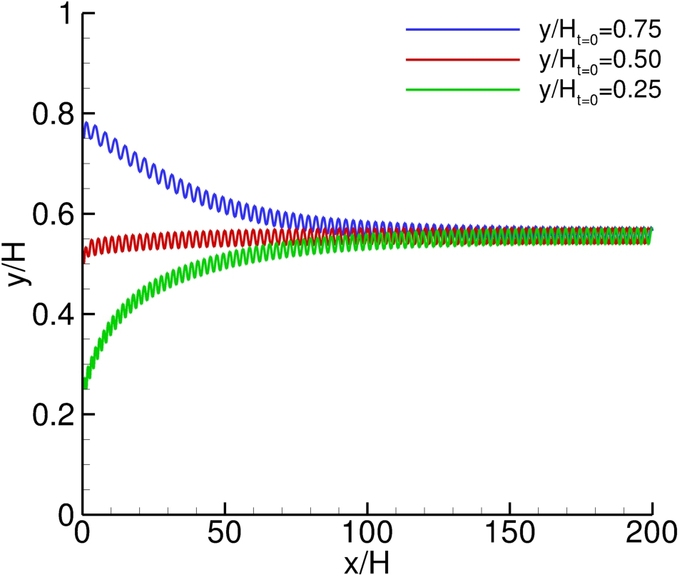
Figure 10 depicts the trajectories of the centroids for square, elliptical and triangular particles. As per the circular particles, the final equilibrium positions, is independent of the initial locations. However, is slightly affected by the particle’s shape. Specifically, for square and elliptical particles just as for the cylindrical particle. Differently, the equilibrium position is for the triangular particle. A weak oscillation around is found in the case of the square particle, see Figure 10(a). This effect increases for elliptical (Figure 10(b)) and triangular particles (Figure 10(c)).
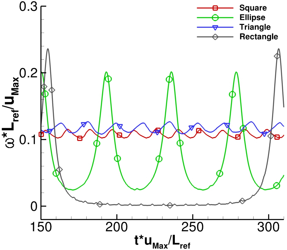
It is now interesting to analyse the particle oscillation around the equilibrium position. The linear velocities, and , shown in Figure 11, behave like in Figure 10, oscillating with different amplitudes and frequencies around the equilibrium position . It is noteworthy that the angular velocity behaviour is determined by the geometrical characteristic of the particle. Indeed, is obtained by solving the Newton’s moment equation, , where is the applied torque and the rotational inertia. In particular, it is confirmed that particles with larger exhibit an increase in oscillation period. Figure 12 shows the comparison between the time variation of obtained considering square, elliptical, triangular, and rectangular particles. The rectangular particle has a major edge length of and an aspect ratio of . The oscillation period is increased from to with an amplitude of about and around the mean value of when the square and the rectangular particle are respectively considered. Moreover, one can observe the different shape of . The triangular and the square particles present a symmetrical oscillation around a certain mean value. On the other hand, the elliptical and rectangular particles present an asymmetry in both, the peak values and the peak width. Precisely, due to the elongated shape of such particles, the oscillation of the angular distribution grows with the ratio between the two main axes of the particle (Figure 12). The elongated shape leads to larger and more peaked velocities. In other words, the peculiar angular velocity distribution, dependent on particles shape and surface, is responsible for the oscillation around the equilibrium position in the linear velocity and consequently in the trajectories of the centre of mass of the particles.
Conclusions and future work
A combined Lattice Boltzmann-Immersed Boundary (LB-IB) model was proposed for predicting the transport dynamics of particles with different shapes, including conventional circular particles as well as less common elliptical, square, rectangular and triangular particles. A comparison between the predictions of the proposed LB-IB method and benchmark results available in the literature for the sedimentation of circular and elliptical cylinders in a quiescent fluid, along with a mesh-refinement study for the latter test case, showed a very good agreement, thus confirming the accuracy of the presented approach. Similarly for the near wall dynamics of a circular cylinder in a linear laminar flow, the LB-IB method was able to predict the complex lateral motion of the particle in agreement with the known results of Joseph and colleagues. Specifically, it was shown that, regardless of the initial location and velocity, the final equilibrium position of the circular cylinder coincides with the middle stream line, with a zero slip linear velocity. At the considered Reynolds number (Re=20), which characterizes the vascular transport of macro-circulation, only minimal differences were observed between the circular and other shaped cylinders. After following qualitatively similar trajectories, square and elliptical cylinders found their equilibrium position on the middle stream line too. Differently, the triangular cylinder reached its equilibrium at 0.53 H. However, the angular velocities show a time-dependent behaviour with amplitude and period significantly affected by the particle shape. Interestingly, beside the expected increase in rotational period, the more elongated particles (elliptical and rectangular) also exhibit a dramatic reduction in the minimum rotational velocity which, for very elongated rectangular particles, would stay at zero for almost the whole period.
It should be here empathised again that the Reynolds number considered (Re=20) in the study would better represent the transport in large vessel of relatively large particles. The actual capillary transport of nanoconstructs would be characterised by significantly smaller Reynolds number (Re). Indeed, the same computational approach here proposed can be readily applied to study transport process at very low Reynolds numbers. Nevertheless, the simulations at Re=20 allowed the authors to validate accurately the model against well known test cases.
Collectively this data demonstrates that the proposed LB-IB approach can be efficiently used for predicting complex particle dynamics in biologically relevant flows. In the near future, three-dimensional simulations at low Reynolds number (Re) of rigid and deformable bodies would help in reproducing and predicting lateral drifting and vascular adhesion of nano/micro-particles at the micro-circulation level. This could provide significant contributions to the field of computational nano-medicine and drug delivery.
Acknowledgement
This project was supported by the European Research Council under the European Union’s Seventh Framework Programme (FP7/2007-2013)/ERC Grant Agreement No. 616695.
References
- [1] D. Peer, J. Karp, S. Hong, O. Farokhzad, R. Margalit, R. Langer, Nanocarriers as an emerging platform for cancer therapy, Nature nanotechnology 2 (2007) 751–60.
- [2] C. Antoniades, C. Psarros, D. Tousoulis, C. Bakogiannis, C. Shirodaria, C. Stefanadis, Nanoparticles: A promising therapeutic approach in atherosclerosis, Current Drug Delivery 7 (4) (2010) 303–311. doi:10.2174/156720110793360586.
- [3] G. Adriani, M. D. de Tullio, M. Ferrari, F. Hussain, G. Pascazio, X. Liu, P. Decuzzi, The preferential targeting of the diseased microvasculature by disk-like particles, Biomaterials 33 (22) (2012) 5504 – 5513. doi:http://dx.doi.org/10.1016/j.biomaterials.2012.04.027.
- [4] A. L. van de Ven, P. Kim, O. Haley, J. R. Fakhoury, G. Adriani, J. Schmulen, P. Moloney, F. Hussain, M. Ferrari, X. Liu, et al., Rapid tumoritropic accumulation of systemically injected plateloid particles and their biodistribution, Journal of Controlled Release 158 (1) (2012) 148–155.
- [5] M. Nabil, P. Decuzzi, P. Zunino, Modelling mass and heat transfer in nano-based cancer hyperthermia, Royal Society Open Science 2 (10). doi:10.1098/rsos.150447.
- [6] P. Decuzzi, R. Pasqualini, W. Arap, M. Ferrari, Intravascular delivery of particulate systems: Does geometry really matter?, Pharmaceutical Research 26 (1) (2009) 235–243. doi:10.1007/s11095-008-9697-x.
- [7] A. C. Anselmo, M. Zhang, S. Kumar, D. R. Vogus, S. Menegatti, M. E. Helgeson, S. Mitragotri, Elasticity of nanoparticles influences their blood circulation, phagocytosis, endocytosis, and targeting, ACS Nano 9 (3) (2015) 3169–3177. doi:10.1021/acsnano.5b00147.
- [8] J. Key, A. Palange, F. Gentile, S. Aryal, C. Stigliano, D. Di Mascolo, E. De Rosa, M. Cho, Y. Lee, J. Singh, P. Decuzzi, Soft discoidal polymeric nanoconstructs resist macrophage uptake and enhance vascular targeting in tumors, ACS Nano 9 (12) (2015) 11628–11641. doi:10.1021/acsnano.5b04866.
- [9] T. J. Merkel, S. W. Jones, K. P. Herlihy, F. R. Kersey, A. R. Shields, M. Napier, J. C. Luft, H. Wu, W. C. Zamboni, A. Z. Wang, J. E. Bear, J. M. DeSimone, Using mechanobiological mimicry of red blood cells to extend circulation times of hydrogel microparticles, Proceedings of the National Academy of Sciences 108 (2) (2011) 586–591. doi:10.1073/pnas.1010013108.
- [10] S. E. A. Gratton, P. A. Ropp, P. D. Pohlhaus, J. C. Luft, V. J. Madden, M. E. Napier, J. M. DeSimone, The effect of particle design on cellular internalization pathways, Proceedings of the National Academy of Sciences 105 (33) (2008) 11613–11618. doi:10.1073/pnas.0801763105.
- [11] P. Decuzzi, S. Lee, M. Decuzzi, M. Ferrari, Adhesion of microfabricated particles on vascular endothelium: A parametric analysis, Annals of Biomedical Engineering 32 (6) (2004) 793–802. doi:10.1023/B:ABME.0000030255.36748.d3.
- [12] S.-Y. Lee, M. Ferrari, P. Decuzzi, Shaping nano-/micro-particles for enhanced vascular interaction in laminar flows, Nanotechnology 20 (49) (2009) 495101.
- [13] T.-R. Lee, M. Choi, A. M. Kopacz, S.-H. Yun, W. K. Liu, P. Decuzzi, On the near-wall accumulation of injectable particles in the microcirculation: smaller is not better, Scientific reports 3.
- [14] S. S. Hossain, T. J. Hughes, P. Decuzzi, Vascular deposition patterns for nanoparticles in an inflamed patient-specific arterial tree, Biomechanics and modeling in mechanobiology 13 (3) (2014) 585–597.
- [15] S. S. Hossain, Y. Zhang, X. Liang, F. Hussain, M. Ferrari, T. J. Hughes, P. Decuzzi, In silico vascular modeling for personalized nanoparticle delivery, Nanomedicine 8 (3) (2013) 343–357.
- [16] P. Decuzzi, B. Godin, T. Tanaka, S.-Y. Lee, C. Chiappini, X. Liu, M. Ferrari, Size and shape effects in the biodistribution of intravascularly injected particles, Journal of Controlled Release 141 (3) (2010) 320–327.
- [17] D. D. Joseph, D. Ocando, Slip velocity and lift, Journal of Fluid Mechanics 454 (2002) 263–286. doi:10.1017/S0022112001007145.
- [18] T.-R. Lee, M. S. Greene, Z. Jiang, A. M. Kopacz, P. Decuzzi, W. Chen, W. K. Liu, Quantifying uncertainties in the microvascular transport of nanoparticles, Biomechanics and modeling in mechanobiology 13 (3) (2014) 515–526.
- [19] M. de Tullio, G. Pascazio, M. Napolitano, Arbitrarily shaped particles in shear flow, ICCFD7 proceedings (1303).
- [20] A. J. C. Ladd, Numerical simulations of particulate suspensions via a discretized boltzmann equation. part 1. theoretical foundation, Journal of Fluid Mechanics 271 (1994) 285–309. doi:10.1017/S0022112094001771.
- [21] A. J. C. Ladd, Numerical simulations of particulate suspensions via a discretized boltzmann equation. part 2. numerical results, Journal of Fluid Mechanics 271 (1994) 311–339. doi:10.1017/S0022112094001783.
- [22] S. Succi, The lattice Boltzmann equation: for fluid dynamics and beyond, Oxford university press, 2001.
- [23] C. Sun, C. Migliorini, L. L. Munn, Red blood cells initiate leukocyte rolling in postcapillary expansions: a lattice boltzmann analysis, Biophysical Journal 85 (1) (2003) 208–222.
- [24] T. Krueger, F. Varnik, D. Raabe, Efficient and accurate simulations of deformable particles immersed in a fluid using a combined immersed boundary lattice boltzmann finite element method, Computers and Mathematics with Applications 61 (12) (2011) 3485 – 3505. doi:http://dx.doi.org/10.1016/j.camwa.2010.03.057.
- [25] M. Vanella, E. Balaras, A moving-least-squares reconstruction for embedded-boundary formulations, Journal of Computational Physics 228 (18) (2009) 6617 – 6628. doi:http://dx.doi.org/10.1016/j.jcp.2009.06.003.
- [26] P. L. Bhatnagar, E. P. Gross, M. Krook, A model for collision processes in gases. i. small amplitude processes in charged and neutral one-component systems, Phys. Rev. 94 (1954) 511–525. doi:10.1103/PhysRev.94.511.
- [27] Y. H. Qian, D. D’Humières, P. Lallemand, Lattice bgk models for navier-stokes equation, EPL (Europhysics Letters) 17 (6) (1992) 479.
- [28] X. Shan, X.-F. Yuan, H. Chen, Kinetic theory representation of hydrodynamics: a way beyond the navier–stokes equation, Journal of Fluid Mechanics 550 (2006) 413–441. doi:10.1017/S0022112005008153.
- [29] J. Latt, B. Chopard, Lattice boltzmann method with regularized pre-collision distribution functions, Mathematics and Computers in Simulation 72 (2006) 165 – 168, discrete Simulation of Fluid Dynamics in Complex Systems. doi:http://dx.doi.org/10.1016/j.matcom.2006.05.017.
- [30] R. Zhang, X. Shan, H. Chen, Efficient kinetic method for fluid simulation beyond the navier-stokes equation, Phys. Rev. E 74 (2006) 046703. doi:10.1103/PhysRevE.74.046703.
- [31] C. E. Colosqui, High-order hydrodynamics via lattice boltzmann methods, Phys. Rev. E 81 (2010) 026702. doi:10.1103/PhysRevE.81.026702.
- [32] Z. Guo, C. Zheng, B. Shi, Discrete lattice effects on the forcing term in the lattice boltzmann method, Phys. Rev. E 65 (2002) 046308. doi:10.1103/PhysRevE.65.046308.
- [33] A. D. Rosis, S. Ubertini, F. Ubertini, A partitioned approach for two-dimensional fluid-structure interaction problems by a coupled lattice boltzmann-finite element method with immersed boundary, Journal of Fluids and Structures 45 (2014) 202 – 215. doi:http://dx.doi.org/10.1016/j.jfluidstructs.2013.12.009.
- [34] K. Suzuki, K. Minami, T. Inamuro, Lift and thrust generation by a butterfly-like flapping wing-body model: Immersed boundary-lattice boltzmann simulations, Journal of Fluid Mechanics 767 (2015) 659–695. doi:10.1017/jfm.2015.57.
- [35] Y. Wang, C. Shu, C. Teo, J. Wu, An immersed boundary-lattice boltzmann flux solver and its applications to fluid-structure interaction problems, Journal of Fluids and Structures 54 (2015) 440 – 465. doi:http://dx.doi.org/10.1016/j.jfluidstructs.2014.12.003.
- [36] J. Favier, A. Revell, A. Pinelli, A lattice boltzmann-immersed boundary method to simulate the fluid interaction with moving and slender flexible objects, Journal of Computational Physics 261 (2014) 145–161. doi:10.1016/j.jcp.2013.12.052.
- [37] Q. Zou, X. He, On pressure and velocity boundary conditions for the lattice boltzmann bgk model, Physics of Fluids 9 (6) (1997) 1591–1598. doi:http://dx.doi.org/10.1063/1.869307.
- [38] C. S. Peskin, The immersed boundary method, Acta Numerica 11 (2002) 479–517. doi:10.1017/S0962492902000077.
- [39] Y. Chen, Q. Cai, Z. Xia, M. Wang, S. Chen, Momentum-exchange method in lattice boltzmann simulations of particle-fluid interactions, Phys. Rev. E 88 (2013) 013303. doi:10.1103/PhysRevE.88.013303.
- [40] O. Filippova, D. Hänel, Grid refinement for lattice-bgk models, Journal of Computational Physics 147 (1) (1998) 219–228. doi:10.1006/jcph.1998.6089.
- [41] R. Mei, W. Shyy, D. Yu, L.-S. Luo, Lattice boltzmann method for 3-d flows with curved boundary, Journal of Computational Physics 161 (2) (2000) 680 – 699. doi:http://dx.doi.org/10.1006/jcph.2000.6522.
- [42]
A. De Rosis, S. Ubertini, F. Ubertini,
A comparison between the
interpolated bounce-back scheme and the immersed boundary method to treat
solid boundary conditions for laminar flows in the lattice boltzmann
framework, Journal of Scientific Computing 61 (3) (2014) 477–489.
doi:10.1007/s10915-014-9834-0.
URL http://dx.doi.org/10.1007/s10915-014-9834-0 - [43] X. Li, F. Jiang, C. Hu, Analysis of the accuracy and pressure oscillation of the lattice boltzmann method for fluid–solid interactions, Computers and Fluids 129 (2016) 33–52.
- [44] J. Yang, E. Balaras, An embedded-boundary formulation for large-eddy simulation of turbulent flows interacting with moving boundaries, Journal of Computational Physics 215 (1) (2006) 12 – 40. doi:http://dx.doi.org/10.1016/j.jcp.2005.10.035.
- [45] Q. Zhang, T. Hisada, Studies of the strong coupling and weak coupling methods in fsi analysis, International Journal for Numerical Methods in Engineering 60 (12) (2004) 2013–2029. doi:10.1002/nme.1034.
- [46] Z. Yu, X. Shao, A direct-forcing fictitious domain method for particulate flows, Journal of Computational Physics 227 (1) (2007) 292 – 314. doi:http://dx.doi.org/10.1016/j.jcp.2007.07.027.
- [47] M. D. de Tullio, G. Pascazio, A moving-least-squares immersed boundary method for simulating the fluid-structure interaction of elastic bodies with arbitrary thickness, Journal of Computational Physics submitted.
- [48] Z. Xia, K. W. Connington, S. Rapaka, P. Yue, J. J. Feng, S. Chen, Flow patterns in the sedimentation of an elliptical particle, Journal of Fluid Mechanics 625 (2009) 249–272. doi:10.1017/S0022112008005521.
- [49] J. Feng, H. H. Hu, D. D. Joseph, Direct simulation of initial value problems for the motion of solid bodies in a newtonian fluid. part 2. couette and poiseuille flows, Journal of Fluid Mechanics 277 (1994) 271–301. doi:10.1017/S0022112094002764.
- [50] G. Fullstone, J. Wood, M. Holcombe, G. Battaglia, Modelling the transport of nanoparticles under blood flow using an agent-based approach, Scientific Reports 5. doi:10.1038/srep10649.
- [51] J. Tan, A. Thomas, Y. Liu, Influence of red blood cells on nanoparticle targeted delivery in microcirculation, Soft Matter 8 (6) (2012) 1934–1946. doi:10.1039/c2sm06391c.
- [52] P. G. Saffman, The lift on a small sphere in a slow shear flow, Journal of Fluid Mechanics 22 (1965) 385–400. doi:10.1017/S0022112065000824.
- [53] F. P. Bretherton, Slow viscous motion round a cylinder in a simple shear, Journal of Fluid Mechanics 12 (1962) 591–613. doi:10.1017/S0022112062000415.