Pairwise Quantization
Abstract
We consider the task of lossy compression of high-dimensional vectors through quantization. We propose the approach that learns quantization parameters by minimizing the distortion of scalar products and squared distances between pairs of points. This is in contrast to previous works that obtain these parameters through the minimization of the reconstruction error of individual points. The proposed approach proceeds by finding a linear transformation of the data that effectively reduces the minimization of the pairwise distortions to the minimization of individual reconstruction errors. After such transformation, any of the previously-proposed quantization approaches can be used. Despite the simplicity of this transformation, the experiments demonstrate that it achieves considerable reduction of the pairwise distortions compared to applying quantization directly to the untransformed data.
1 Introduction
Approaches based on quantization with multiple codebooks (such as product quantization [10], residual quantization [3], optimized product quantization [7, 12], additive quantization [1], composite quantization [16], tree quantization [2]) perform lossy compression of high-dimensional vectors, achieving very good trade-off between accuracy at preserving the high-dimensional vectors, speed, and compression ratio. In many scenarios associated with machine learning and information retrieval, one is interested to preserve the pairwise relations between high-dimensional points (e.g. distances, scalar products) rather than the points themselves. This is not reflected in the existing quantization approaches, which invariably learn their parameters (e.g. codebooks) from data by minimizing the reconstruction (compression) error of the training data points.
In this work, we aim to derive quantization-based methods that directly minimize distortions of pairwise relations between points rather than reconstruction errors of individual points. In particular, we focus on minimizing the distortion of scalar products and squared Euclidean distances between uncompressed and compressed that might come from two different distributions. This case is important for two reasons. Firstly, it is often beneficial (in terms of accuracy) to compress only one argument (e.g. when one needs to evaluate distances between a user query and a large dataset of points, there is no need to compress vectors expressing user queries). Secondly, quantization-based methods are particularly efficient at evaluating pairwise relations between compressed and uncompressed points as they can use the asymmetric distance computation (ADC) scheme [10]. Given an uncompressed and a very large dataset of compressed vectors , the ADC scheme precomputes the look-up tables containing the distances between and the codewords, and then does a linear scan through compressed vectors while estimating distances or scalar products by summing up values from the look-up tables.
Our approach proceeds by reducing the task of minimizing the pairwise relation distortions to the original task of minimizing the reconstruction error of individual points. We demonstrate that both for scalar products and for pairwise distances, such reduction can be achieved through simple linear transforms estimated from data. After such transforms, any of the existing quantization schemes [10, 3, 7, 12, 1, 16, 2] can be applied. In the experiments, we demonstrate that applying the proposed transform allows to reduce the quantization-induced distortions of pairwise relations very considerably, as compared to applying quantization to the original vectors.
We discuss several practical applications where this improvement can matter for scalar products. For squared Euclidean distances, we find that our approach is dominated by large distances and hence is only beneficial when preserving long distances (rather than distances between close neighbors) matter.
2 Review of Vector and Product Quantization
Since the topic of this paper is vector quantization, and as our method relies heavily on existing vector quantization approaches (Section 3), here we provide a brief overview of a state-of-the-art approach called Optimized Product Quantization (OPQ) [7, 12].
The goal of all existing vector quantization methods is to represent vectors well while achieving large compression rates, i.e. for a given memory budget and training vectors , one wants to quantize them such that their reconstructions achieve the minimal quantization error:
| (1) |
As will be shown in Sections 3.1 and 3.2, methods which minimize quantization distortions are suboptimal when it comes to the task of achieving best scalar product or squared Euclidean distance estimates.
A method which directly minimizes the quantization distortion is k-means. Thus, a codebook of size is learnt using k-means and each vector is approximated using its nearest codeword, i.e. the assignment of vector is done using and the ID of the nearest codeword is used for the compressed representation of the vector, giving rise to a -bit representation. The approximated version of is then the closest codeword itself .
Given a large dataset , a memory-efficient way of computing an approximate value of any scalar function for all the vectors is: (i) off-line stage: compress all database vectors and store their IDs , (ii) online stage: compute for each in , and then simply look up this value for each compressed database vector: . For example, given a compressed database , such a system is able to quickly estimate a scalar product between any query vector and the entire database by pre-computing all and then looking up these values .
However, this method is impractical in real life situations as for moderate and large bitrates one would require prohibitively large codebooks, e.g. for 32 bits and 64 bits the codebook would contain 4 billion and vectors, respectively. This is impractical as (i) it is impossible to learn such a large codebook in terms of computation time and lack of training data, (ii) storing the codebook would require a huge amount of memory, and (iii) encoding vectors and (iv) pre-computing for all would be too slow.
Product Quantization (PQ).
Jégou et al. [10] and subsequent related methods [3, 7, 12, 1, 2], follow the k-means approach but address its deficiencies by means of a “product vocabulary” – a vector is split into non-overlapping block where each block is quantized independently with its own k-means-based quantizer. The compressed representation of the vector is now the -tuple of IDs of the closest codewords for each block: , where be the -th block of vector and .
The size of the quantized representation is and the number of distinct vectors which can be obtained using this coding scheme is , while the number of codewords which should be learnt is only . PQ makes it possible to use larger codes than the naive k-means method, e.g. to achieve a 64-bit code one can use and , requiring only codewords to be learnt from the data, as opposed to k-means which would require .
On the other hand, due to the structure imposed onto the “product vocabulary”. it is not possible any more to evaluate arbitrary functions in the same manner as before. However, many useful functions are decomposable over blocks of the input vector and can therefore be evaluated with PQ, with notable examples being the scalar product and the squared Euclidean distance. It is possible to estimate the scalar product between a query vector and any quantized vector as follows:
| (2) |
Similarly to the k-means case, for a new query vector , one can pre-compute the scalar products for each block and each codeword of that block (done in ) and store them in a lookup table. Then, it is possible to estimate the scalar product between the query and all compressed database vectors by simply summing up the scalar product contributions of each block (done in per database vector). A completely analogous strategy can be used to estimate the squared Euclidean distances as it also decomposes into a sum of per-block squared Euclidean distances.
The original paper [10] analyzed the effect of product quantization on pairwise distance estimates and found out that PQ has a shrinking effect thus giving biased estimates. They have also suggested an additive factor that leads to an unbiased estimate; we explore this topic in more detail in Section 3.3.
Optimized Product Quantization (OPQ).
Due to the splitting of input vectors into blocks, PQ is not invariant to rotations of the vector space, i.e. different rotations of the space can yield different compression quality. To address this issue, Ge et al. [7] and Norouzi and Fleet [12] propose two very similar methods, which hereafter we jointly refer to as OPQ. Namely, OPQ aims at finding the best rotation such that compressing with PQ yields the smallest distortion; the quantization and rotation are learnt from training vectors by alternating between learning PQ in a fixed rotated space with learning the best rotation under the fixed PQ. The computation of the scalar product or the squared Euclidean distance between a query vector and the compressed database is the same as above for PQ, apart from a simple preprocessing step where each vector is rotated by .
3 The approach
In general, we consider squared distances and scalar products between uncompressed query vectors and compressed dataset vectors . We assume that these two vectors come from the two distributions and , and we assume that at training time we are given datasets of vectors and coming from these distributions. Note, that we do not assume any similarity between and .
We now derive the transformations that allows to apply standard quantization methods in a way that the expected distortions of pairwise relations between and are minimized. We start with the scalar products and then extend the construction to squared Euclidean distances.
3.1 Scalar products
We are interested in efficiently computing the scalar product for all , and to achieve this, we seek to obtain the approximate representations for the dataset vectors, which will facilitate the efficient approximate scalar product estimation. Given a training set of query vectors , the task is to minimize the square loss between the real scalar products and the scalar product estimates:
| (3) |
Further manipulations reveal:
| (4) |
Defining gives:
| (5) |
Note that is a positive semi-definite matrix as it is a sum of positive semi-definite matrices , so it is possible to use SVD to decompose it into such that . One can now define a mapping of vectors into by , and , yielding the loss:
| (6) |
By means of the aforementioned mapping, we have reduced the original problem to the standard problem of vector quantization (c.f. (1)) in the transformed -space, where the goal is to minimize mean squared error between the original vectors and the vector reconstructions. Any vector quantization method can be used here, and we employ Optimized Product Quantization (c.f. Section 2 for a review).
At query time, to estimate the scalar product between a query and a database vector , we simply reverse the above order of operations, i.e. the reconstructed are obtained from by inverting the transformation :
| (7) |
where is the (pseudo)inverse of .
Note that at query time it is not actually necessary to explicitly reconstruct as OPQ can efficiently compute a scalar product between an uncompressed vector (here ) and a quantized vector (compressed representation of ) using additions of values from a lookup table; for more details on OPQ, recall Section 2.
3.2 Squared Euclidean distances
Analogously to the scalar product preservation task from the previous section, here we consider the task of efficiently estimating the squared Euclidean distances between the query and the database vectors . We seek to obtain the approximate database vector representations to minimize the square loss between real and estimated squared distances:
| (8) |
Expanding the inner squares gives:
| (9) |
Consider the following definition of vectors and : and , simplifying the expression for the loss to:
| (10) |
Comparing (10) to (3) it is clear that the Euclidean distance preservation problem has been reduced to the scalar product preservation problem. Namely, the -matrix is formed as and SVD is applied to obtain the transformation matrix (a matrix square root of ). The -vectors are then formed as and the task is again reduced to minimizing , for which we again employ OPQ.
At query time, to estimate the squared distance between a query and a database vector , we follow the procedure analogous to the scalar product one:
| (11) |
3.3 Estimation bias
In this section we show that our methods provide unbiased estimates for the scalar product and the squared Euclidean distance, while OPQ and other vector quantization methods are only unbiased when used for the scalar product approximation.
For a given query vector , we are interested in the difference in the expected values of the scalar function and its estimator which uses the approximate version of , where , i.e.:
| (12) |
We start by investigating the OPQ estimation bias, and then use the derived results to analyze our Pairwise Quantization.
3.3.1 Optimized Product Quantization
Since the computations of the scalar product and the squared Euclidean distance decompose across quantization blocks for (Optimized) Product Quantization (i.e. the scalar product estimate is the sum over scalar product estimates over all quantization blocks), it is sufficient to consider the single quantization block case () without loss of generality. For this setting, learning the OPQ codebook corresponds to performing k-means on all training vectors, while the quantization is performed by simply assigning the vector to the nearest cluster centre: . The approximation of is then . To evaluate the estimation bias, if will be beneficial to do so on a per-cluster basis, i.e. the bias will be computed for all assigned to a particular cluster centre :
| (13) |
Then the overall bias can be computed as:
| (14) |
which is a weighted sum of the per-cluster biases.
Scalar product.
The function of interest is . As is a constant independent of it straightforwardly follows that:
| (15) |
where the last equality comes from the fact that from the definition of the k-means algorithm (i.e. the cluster centre is the mean of the vectors assigned to it). As all per-cluster biases are equal to zero, and the overall bias is a weighted sum of per-cluster biases, the overall bias is zero as well, so OPQ produces an unbiased estimate of the scalar product.
Squared Euclidean distance.
Investigation of the bias of squared Euclidean distance estimates of (O)PQ has already been performed in the original PQ paper [10], but we include it here for completeness.
The function of interest is . Using again the fact that , the expected squared distance for a given cluster is:
| (16) | |||||
| (17) | |||||
| (18) | |||||
| (19) | |||||
| (20) | |||||
| (21) |
As is the estimate of the squared distance, the per-cluster bias is therefore . This term corresponds to the mean squared error (MSE) and is in general larger than zero. Since the overall bias is a weighted sum of per-cluster biases, where the weights are all non-negative and in general larger than zero, the overall bias is larger than zero. Therefore, OPQ produces a biased estimate for the squared Euclidean distance, and it on average provides an underestimate.
For the case where there are more than one subquantizers (), since the squared distance estimates are additive, it is easy to show that the bias correction term is equal to the sum of the individual MSE’s [10].
Generalization to other methods.
Other popular methods for vector quantization such as Residual Vector Quantization (RVQ) [3], Additive Quantization (AQ) [1], Tree Quantization (TQ) [2], and Composite Quantization (CQ) [16] are all equivalent to OPQ when the number of subquantizers is and therefore in general yield biased squared Euclidean distance estimates. Regarding the scalar product estimates – RVQ is unbiased, which can be proven in the same way as for OPQ, while for the more involved methods AQ, TQ and CQ it is not clear whether they are biased or not.
3.3.2 Pairwise Quantization
Scalar product.
Recall from Section 3.1 and (7) that and that therefore the scalar product is . Defining , the estimator bias is:
| (22) |
As the right hand side corresponds to the bias of the scalar product estimates in the z-space, the bias of our method depends on the underlying method we choose to use in the z-space. Since we use OPQ which, as shown earlier, yields unbiased estimates of the scalar product, our method is also unbiased.
Squared Euclidean distance.
As shown in Section 3.2, by introducing new variables and , the squared Euclidean distance can be computed as a sum of a constant and a scalar product . Since our method provides unbiased estimates of the scalar product, it is clear that the squared Euclidean distance estimates are unbiased as well. Note that this is different from OPQ which yields biased estimators.
4 Applications and experiments
Now we demonstrate the advantage of Pairwise Quantization (PairQ) on real datasets from three different applications. In all experiments below we use OPQ to perform compression (6) and also use OPQ as the main baseline for comparison unless stated otherwise. For both OPQ and PairQ we use codebooks with codewords which is a standard choice in most previous works.
4.1 Text-to-image retrieval
The problem of text-to-image retrieval arises in image search engines that rank images based on their relevance to a user text query. The advanced methods for this problem typically use multimodal deep neural networks that learn common representations for both text and images capturing the semantics of both modalities [6]. Given such representations, the relevance of a particular image to a particular text query is measured as a cosine similarity between them, i.e. the scalar product of the L2-normalized features.
The retrieval quality can be improved by using images metadata (e.g. tags, EXIF, etc.). Therefore, modern search engines combine the relevance score provided by the deep representations with features extracted from the metadata via a higher-level ranker that re-orders images based on multiple sources of information. For large image databases, exact evaluation of all cosine distances for a given query is expensive, hence approximate evaluation is used in practice. Clearly, it is important to minimize the corruption of cosine distance values in order to provide good features to the higher-level ranker. We compare OPQ and PairQ for this problem and measure the average squared error of cosine distance approximations for both methods.
We followed the protocol described in [6] and trained a multimodal deep network on a set of text-image pairs. The train dataset was collected by ourselves via querying an image search engine with popular text queries. For each query we used the top ten images as positives (their relevance to the query equals one) and random images from the web as negatives (their relevance to the query equals zero). After the network was learnt, we computed the representations for images and text queries. The dimensionality of the representations was set to . The dataset is available upon request11 1 Please contact Artem Babenko at artem.babenko@phystech.edu.
In this experiment we used image representations for learning OPQ and PairQ codebooks as well as the rotation matrices inside OPQ. The other image representations were used for performance evaluation. To learn the transformation in PairQ we used text representations and the remaining text representations were used only for the performance evaluation of both methods.
| Bytes per vector | 5 | 10 | 20 | 25 | 50 |
| Compression ratio | 80 | 40 | 20 | 16 | 8 |
| OPQ error, | 2.127 | 1.234 | 0.508 | 0.356 | 0.056 |
| PairQ error, | 1.764 | 0.961 | 0.329 | 0.203 | 0.045 |
| Error reduction w.r.t OPQ | 17% | 22% | 35% | 43% | 20% |
The results of comparison are presented in Table 1. We used different numbers of codebooks for both OPQ and PairQ thus providing different compression ratios, corresponding to different memory and time budgets. Table 1 demonstrates that PairQ outperforms OPQ over the whole range of compression ratios, and reduces OPQ error by upto .
4.2 Recommendation systems
Recommendation systems have become ubiquitous on e-commerce sites where the task is to suggest items to users according to their personal preferences. This problem is typically solved by collaborative filtering (CF) methods that perform a factorization of the user ratings matrix thus producing latent vector representations for each user and each item . Then the relevance of an item to a specific user can be obtained as the value of the scalar product . The alternative approach to the personalization problem is to use content-based filtering (CBF) that is based on given descriptions of users and items (e.g. tags, clicks, user history, etc.).
The modern systems typically combine both approaches and use the outputs of CF and CBF as features for a higher-level recommender [8]. Hence to produce recommendations for a user with a latent representation , the scalar products should be computed, where is the items database. For large , the exact evaluation of scalar products can be computationally expensive and efficient approximate methods should be used. Along with efficiency, approximate methods should provide accurate reconstructions of scalar product values that will be then used by the higher-level recommender. We compare OPQ and PairQ for this problem of approximate scalar product evaluation and use the average squared error of approximation as the performance measure.
We perform the comparison on the well-known MovieLens-20M dataset [9]. Latent user and item representations of dimensionality were obtained by the standard PureSVD procedure [4]. Overall this dataset contains user vectors and item vectors. We used the first user vectors to learn the transformation and the other user vectors to evaluate the approximation quality.
| Bytes per vector | 5 | 10 | 15 | 25 | 50 |
| Compression ratio | 120 | 60 | 40 | 24 | 12 |
| OPQ error, | 7.570 | 6.952 | 5.828 | 4.432 | 1.793 |
| PairQ error, | 6.464 | 4.601 | 3.719 | 2.529 | 1.297 |
| Error reduction w.r.t OPQ | 15% | 34% | 36% | 42% | 28% |
We provide the results of comparison for different compression ratios in Table 2. It shows that PairQ provides significantly more accurate scalar product approximations than OPQ. For instance, the usage of PairQ instead of OPQ allows to reduce the squared approximation error by .
4.3 Preserving Euclidean distances
Many machine learning algorithms require efficient evaluation of Euclidean distances between a given query and a large number of database vectors. Several examples are large-scale SVMs with RBF kernel, kernelized regression and non-parametric density estimation. We show that Pairwise Quantization provides more accurate reconstructions of Euclidean distances comparing to OPQ for the same runtime and memory costs.
The experiments were performed on three datasets. The SIFT1M dataset [10] contains one million of -dimensional SIFT descriptors [11] along with predefined queries. The GIST1M dataset [10] contains one million of -dimensional GIST descriptors [13] and queries. The DEEP1M dataset [2] contains one million of -dimensional deep descriptors and queries. Deep descriptors are formed as PCA-compressed outputs from a fully-connected layer of a CNN pretrained on the Imagenet dataset [5].
 |
 |
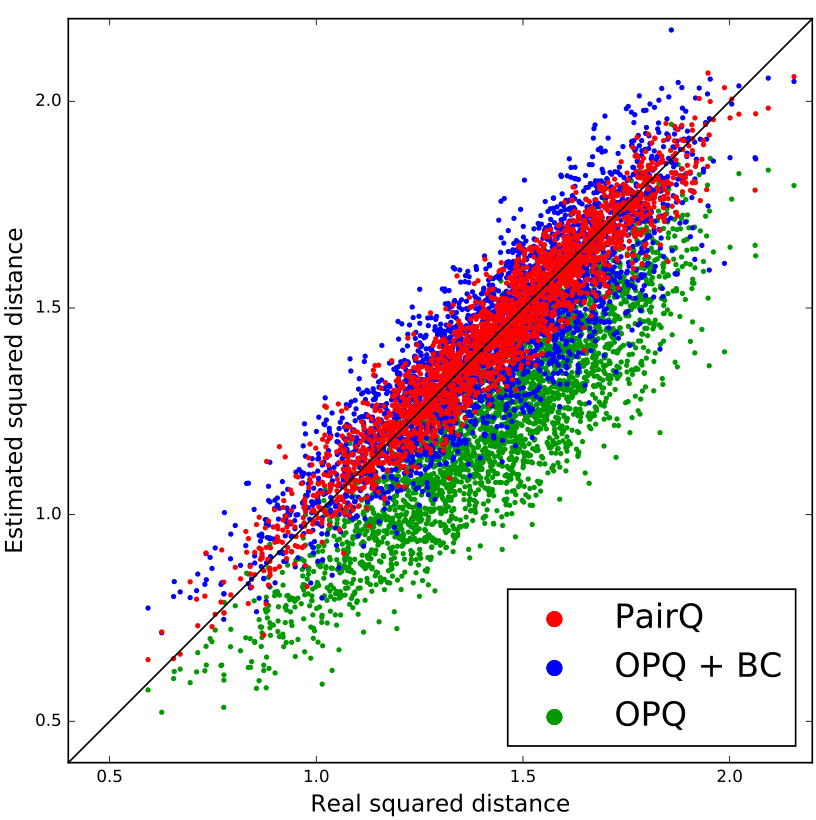 |
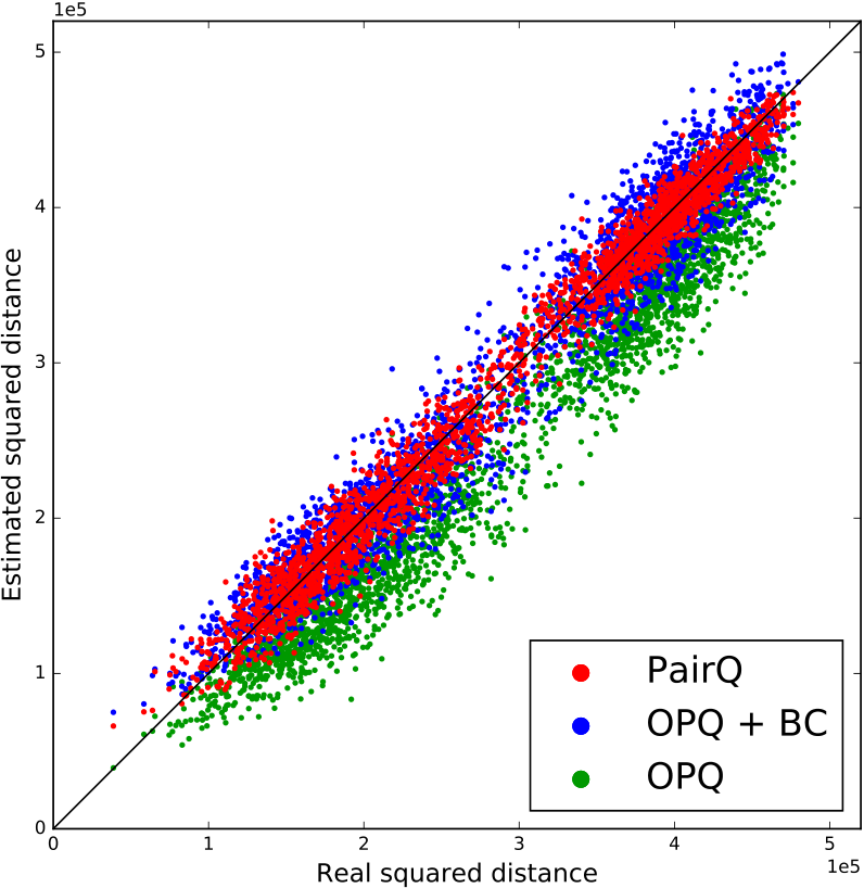
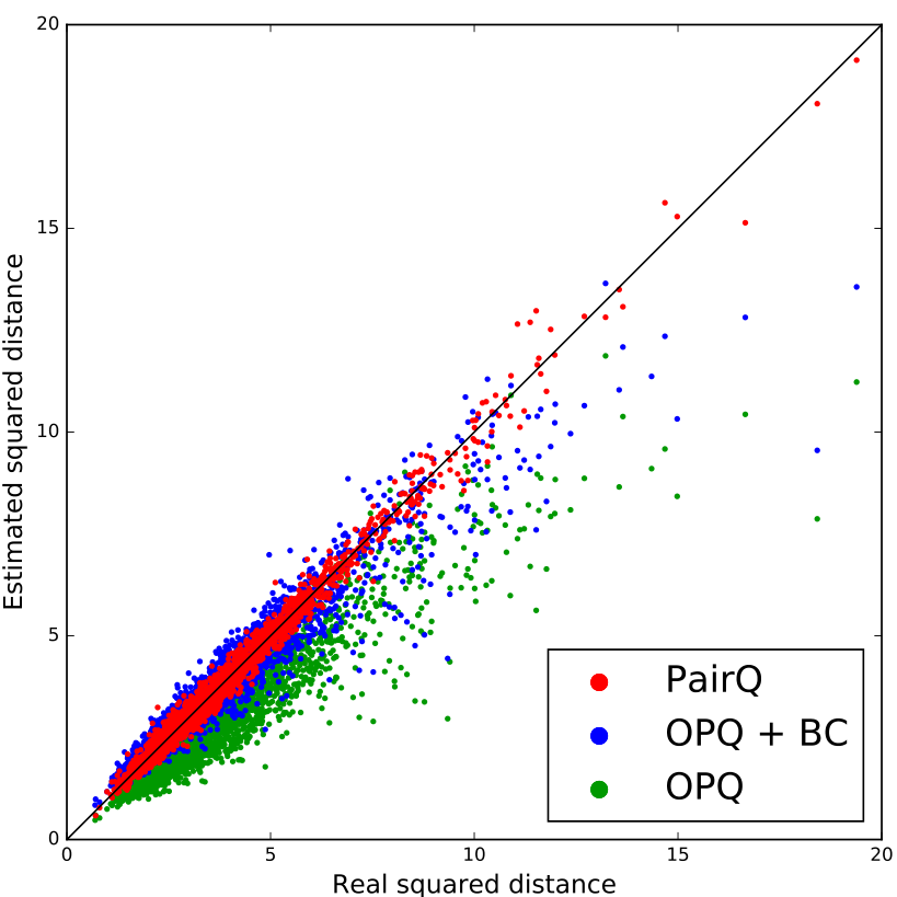
Along with OPQ as the first baseline, we also include OPQ with bias correction (OPQ+BC) as the second baseline. The bias correction term is computed as described in (21) and provides more accurate distance estimation as we show below. For all datasets, the codebooks for OPQ and PairQ and the transformation in PairQ are learnt on the provided hold-out sets.
For each query and each database vector we evaluate a relative approximation error of the Euclidean distance produced by OPQ, OPQ+BC and PairQ. Figure 1 (top row) shows relative errors averaged over all possible pairs and for different memory budgets per vector. For all datasets PairQ significantly outperforms OPQ and OPQ with bias correction. Note, PairQ requires several times less memory per vector to provide the same accuracy, e.g. the performance of PairQ with four bytes per vector is on par with the performance of OPQ with 16 bytes per vector.
We also experimented with the usage of PairQ for the approximate nearest neighbor search problem. For this application PairQ provided inferior results on all datasets comparing to OPQ. The reason for the low performance of PairQ here is that the functional (8) puts too much emphasis on the distant point pairs while only the close pairs are important for ANN search. A similar effect (better distance estimates but worse ANN performance) was noticed in [10] for their bias correction procedure.
5 Summary
We have proposed a new approach for quantization methods that proceeds by minimizing distortions of pairwise relations on the training set. This is in contrast to previous works that optimize the reconstruction error of individual points. We develop a simple technique based on linear transformation that allows to reduce the task of minimizing pairwise distortions to the task of minimizing the reconstruction error in the transformed space. This allows us to adapt previously proposed quantization methods to minimize pairwise distortions directly.
The experiments confirm that our approach achieves significant reduction in pairwise distortions, when squared distances and scalar product between compressed and uncompressed vectors are considered. We note that beyond retrieval and recommendation systems, the improvement in scalar product estimation accuracy can be useful for learning classifiers and detectors in a large-scale setting [14, 15]. Finally, we note that our method is almost straightforwardly applicable beyond quantization, and can turn any learning-based lossy compression method that optimizes the reconstruction error into a method that minimizes expected pairwise distortion. We plan to investigate this ability further in future work.
Acknowledgements.
Relja Arandjelović is supported by the ERC grant LEAP (no. 336845). Victor Lempitsky is supported by the Russian Ministry of Science and Education grant RFMEFI61516X0003.
References
- [1] A. Babenko and V. Lempitsky. Additive quantization for extreme vector compression. CVPR, 2014.
- [2] A. Babenko and V. Lempitsky. Tree quantization for large-scale similarity search and classification. CVPR, 2015.
- [3] Y. Chen, T. Guan, and C. Wang. Approximate nearest neighbor search by residual vector quantization. Sensors, 10(12):11259–11273, 2010.
- [4] P. Cremonesi, Y. Koren, and R. Turrin. Performance of recommender algorithms on top-n recommendation tasks. Proceedings of the 2010 ACM Conference on Recommender Systems, RecSys 2010, Barcelona, Spain, September 26-30, 2010, pp. 39–46, 2010.
- [5] J. Deng, W. Dong, R. Socher, L.-J. Li, K. Li, and L. Fei-Fei. Imagenet: A large-scale hierarchical image database. CVPR, 2009.
- [6] H. Fang, S. Gupta, F. N. Iandola, R. K. Srivastava, L. Deng, P. Dollár, J. Gao, X. He, M. Mitchell, J. C. Platt, C. L. Zitnick, and G. Zweig. From captions to visual concepts and back. IEEE Conference on Computer Vision and Pattern Recognition, CVPR 2015, Boston, MA, USA, June 7-12, 2015, pp. 1473–1482, 2015.
- [7] T. Ge, K. He, Q. Ke, and J. Sun. Optimized product quantization for approximate nearest neighbor search. CVPR, 2013.
- [8] A. Gunawardana and C. Meek. A unified approach to building hybrid recommender systems. Proceedings of the 2009 ACM Conference on Recommender Systems, RecSys 2009, New York, NY, USA, October 23-25, 2009, pp. 117–124, 2009.
- [9] F. M. Harper and J. A. Konstan. The movielens datasets: History and context. TiiS, 5(4):19, 2016.
- [10] H. Jégou, M. Douze, and C. Schmid. Product quantization for nearest neighbor search. TPAMI, 33(1), 2011.
- [11] D. G. Lowe. Distinctive image features from scale-invariant keypoints. IJCV, 60(2), 2004.
- [12] M. Norouzi and D. J. Fleet. Cartesian k-means. CVPR, 2013.
- [13] A. Oliva and A. Torralba. Modeling the shape of the scene: A holistic representation of the spatial envelope. IJCV, 42(3), 2001.
- [14] J. Sánchez and F. Perronnin. High-dimensional signature compression for large-scale image classification. CVPR, pp. 1665–1672, 2011.
- [15] A. Vedaldi and A. Zisserman. Sparse kernel approximations for efficient classification and detection. CVPR, pp. 2320–2327, 2012.
- [16] T. Zhang, C. Du, and J. Wang. Composite quantization for approximate nearest neighbor search. ICML, 2014.