Efficient tensor completion for color image and video recovery: Low-rank tensor train
Abstract
This paper proposes a novel approach to tensor completion, which recovers missing entries of data represented by tensors. The approach is based on the tensor train (TT) rank, which is able to capture hidden information from tensors thanks to its definition from a well-balanced matricization scheme. Accordingly, new optimization formulations for tensor completion are proposed as well as two new algorithms for their solution. The first one called simple low-rank tensor completion via tensor train (SiLRTC-TT) is intimately related to minimizing a nuclear norm based on TT rank. The second one is from a multilinear matrix factorization model to approximate the TT rank of a tensor, and is called tensor completion by parallel matrix factorization via tensor train (TMac-TT). A tensor augmentation scheme of transforming a low-order tensor to higher-orders is also proposed to enhance the effectiveness of SiLRTC-TT and TMac-TT. Simulation results for color image and video recovery show the clear advantage of our method over all other methods.
Index Terms:
Color image recovery, video recovery, tensor completion, tensor train decomposition, tensor train rank, tensor train nuclear norm, Tucker decomposition.The authors are from the Faculty of Engineering and Information Technology, University of Technology Sydney, Ultimo, NSW 2007, Australia.
E-mail: ngocphien.ho@uts.edu.au, tuan.hoang@uts.edu.au.
I Introduction
Tensors are multi-dimensional arrays, which are higher-order generalizations of matrices and vectors [1]. Tensors provide a natural way to represent multidimensional data whose entries are indexed by several continuous or discrete variables. Employing tensors and their decompositions to process data has become increasingly popular since [2, 3, 4]. For instance, a color image is a third-order tensor defined by two indices for spatial variables and one index for color mode. A video comprised of color images is a fourth-order tensor with an additional index for a temporal variable. Residing in extremely high-dimensional data spaces, the tensors in practical applications are nevertheless often of low-rank [1]. Consequently, they can be effectively projected to much smaller subspaces through underlying decompositions such as the CANDECOMP/PARAFAC (CP)[5, 6], Tucker [7] and tensor train (TT) [8] or matrix product state (MPS)[9, 10, 11].
Motivated by the success of low rank matrix completion (LRMC) [12, 13, 14], recent effort has been made to extend its concept to low rank tensor completion (LRTC). In fact, LRTC has found applications in computer vision and graphics, signal processing and machine learning [15, 16, 17, 18, 19, 20, 21]. The common target is to recover missing entries of a tensor from its partially observed entities [22, 23, 24]. LRTC remains a grand challenge due to the fact that computation for the tensor rank, defined as CP rank, is already an NP-hard problem [1]. There have been attempts in approaching LRTC via Tucker rank [15, 18, 21]. A conceptual drawback of Tucker rank is that its components are ranks of matrices constructed based on an unbalanced matricization scheme (one mode versus the rest). The upper bound of each individual rank is often small and may not be suitable for describing global information of the tensor. In addition, the matrix rank minimizations is only efficient when the matrix is more balanced. As the rank of a matrix is not more than , where and are the number of rows and columns of the matrix, respectively, the high ratio would effectively rule out the need of matrix rank minimization. It is not surprising for present state-of-the-art LRMC methods [25, 26, 12, 13] to implicitly assume that the considered matrices are balanced.
Another type of tensor rank is the TT rank, which constitutes of ranks of matrices formed by a well-balanced matricization scheme, i.e. matricize the tensor along permutations of modes. TT rank was defined in [8], yet low rank tensor analysis via TT rank can be seen in earlier work in physics, specifically in simulations of quantum dynamics [27, 28]. Realizing the computational efficiency of low TT rank tensors, there has been numerous works in applying it to numerical linear algebra [29, 30, 31]. Low TT rank tensors were used for the singular value decomposition (SVD) of large-scale matrices in [32, 33]. The alternating least squares (ALS) algorithms for tensor approximation [34, 35] are also used for solutions of linear equations and eigenvector/eigenvalue approximation. In [36, 37], low TT rank tensors were also used in implementing the steepest descent iteration for large scale least squares problems. The common assumption in all these works is that all the used tensors during the computation processes are of low TT rank for computational practicability. How low TT rank tensors are relevant to real-world problems was not really their concern. Applications of the TT decomposition to fields outside of mathematics and physics has rarely been seen, with only a recent application of TT to machine learning [38]. As mentioned above, color image and video are perfect examples of tensors, so their completion can be formulated as tensor completion problems. However, it is still not known if TT rank-based completion is useful for practical solutions. The main purpose of this paper is to show that TT rank is the right approach for LRTC, which can be addressed by TT rank-based optimization. The paper contribution is as follows:
- 1.
Using the concept of von Neumann entropy in quantum information theory [39], we show that Tucker rank does not capture the global correlation of the tensor entries and thus is hardly ideal for LRTC. Since TT rank constitutes of ranks of matrices formed by a well-balanced matricization scheme, it is capable of capturing the global correlation of the tensor entries and is thus a promising tool for LRTC.
- 2.
We show that unlike Tucker rank, which is often low and not interesting for optimization, TT rank optimization is a tractable formulation for LRTC. Two new algorithms are introduced to address the TT rank optimization based LRTC problems. The first algorithm called simple low-rank tensor completion via tensor train (SiLRTC-TT) solves an optimization problem based on the TT nuclear norm. The second algorithm called tensor completion by parallel matrix factorization via tensor train (TMac-TT) uses a mutilinear matrix factorization model to approximate the TT rank of a tensor, bypassing the computationally expensive SVD. Avoiding the direct TT decomposition enables the proposed algorithms to outperform other start-of-the-art tensor completion algorithms.
- 3.
We also introduce a novel technique called ket augmentation (KA) to represent a low-order tensor by a higher-order tensor without changing the total number of entries. The KA scheme provides a perfect means to obtain a higher-order tensor representation of visual data by maximally exploring the potential of TT rank-based optimization for color image and video completion. TMac-TT especially performs well in recovering videos with missing entries.
The rest of the paper is organized as follows. Section II introduces notation and a brief review of tensor decompositions. In Section III, the conventional formulation of LRTC is reviewed, the advantage of TT rank over Tucker rank in terms of global correlations is discussed, then the proposed reformulations of LRTC in the concept of TT rank. Section IV introduces two algorithms to solve the LRTC problems based on TT rank, followed by a discussion of computational complexity. Subsequently, the tensor augmentation scheme known as KA is proposed in Section V. Section VI provides experimental results and finally, we conclude our work in Section VII.
II Tensor ranks
Some mathematical notations and preliminaries of tensors are adopted from [1]. A tensor is a multi-dimensional array and its order or mode is the number of its dimensions. Scalars are zero-order tensors denoted by lowercase letters . Vectors and matrices are the first- and second-order tensors which are denoted by boldface lowercase letters (x, y, z,…) and capital letters , respectively. A higher-order tensor (the tensor of order three or above) are denoted by calligraphic letters .
An Nth-order tensor is denoted as where , is the dimension corresponding to mode . The elements of are denoted as , where , . The Frobenius norm of is .
A mode- fiber of a tensor is a vector defined by fixing all indices but and denoted by x.
Mode- matricization (also known as mode- unfolding or flattening) of a tensor is the process of unfolding or reshaping the tensor into a matrix by rearranging the mode- fibers to be the columns of the resulting matrix. Tensor element maps to matrix element such that
| (1) |
The vector , where is the rank of the corresponding matrix denoted as , is called as the Tucker rank of the tensor . It is obvious that .
Using Vidal’s decomposition [28], can be represented by a sequence of connected low-order tensors in the form
| (2) |
where for , is an matrix and is the diagonal singular matrix, . For every , the following orthogonal conditions are fulfilled:
| (3) | |||||
| (4) |
where and are the identity matrices of sizes and , respectively. The TT rank of the tensor is simply defined as , and can be determined directly via the singular matrices . Specifically, to determine , rewrite (2) as
| (5) |
where
| (6) |
and
| (7) |
We can also rewrite (5) in terms of the matrix form of an SVD as
| (8) |
where () is the mode- matricization of the tensor [8], and are orthogonal matrices. The rank of is , which is defined as the number of nonvanishing singular values of .
Since matrix is obtained by matricizing along modes, its rank is bounded by .
III Tensor completion
This section firstly revisits the conventional formulation of LRTC based on the Tucker rank. Then, we propose a new approach to LRTC via TT rank optimization, which leads to two new optimization formulations, one based on nuclear norm minimization, and the other on multilinear matrix factorization.
III-A Conventional tensor completion
As tensor completion is fundamentally based on matrix completion, we give an overview of the latter prior its introduction. Recovering missing entries of a matrix from its partially known entries given by a subset can be studied via the well-known matrix-rank optimization problem [40, 41]:
| (9) |
The missing entries of are completed such that the rank of is as small as possible, i.e the vector of the singular values of is as sparse as possible. The sparsity of leads to the effective representation of for accurate completion. Due to the combinational nature of the function , the problem (9), however, is NP-hard. For the nuclear norm , the following convex optimization problem in has been proved the most effective surrogate for (9) [25, 12, 13]:
| (10) |
It should be emphasized that the formulation (9) is efficient only when is balanced (square), i.e. . It is likely that for unbalanced with , i.e. there is not much difference between the optimal value of (9) and its upper bound , under which rank optimization problem (9) is not interesting. More importantly, one needs at least sampled entries [26] with a positive constant to successfully complete , which is almost the total entries of .
Completing an th-order tensor from its known entries given by an index set is formulated by the following Tucker rank optimization problem [15, 18, 20, 21]:
| (11) |
where are defined as weights fulfilling the condition , which is then addressed by the following optimization problem [15]:
| (12) |
Each matrix in (11) is obtained by matricizing the tensor along one single mode and thus is highly unbalanced. For instance, when all the modes have the same dimension (), its dimension is . As a consequence, its rank is low, which makes the matrix rank optimization formulation (11) less efficient for completing . Moreover, as analyzed above, it also makes the optimization problem (12) not efficient in addressing the rank optimization problem (11).
In the remainder of this subsection we show that is not an appropriate means for capturing the global correlation of a tensor as it provides only the mean of the correlation between a single mode (rather than a few modes) and the rest of the tensor.
Firstly, normalize () and represent it as:
| (13) |
where “” denotes a tensor product [1], form an orthonormal basis in for each . Applying mode- matricization of results in representing a pure state of a composite system in the space , which is a tensor product of two subspaces and of dimensions and , respectively. The subsystems and are seen as two contigous partitions consisting of mode and all other modes of the tensor, respectively. It follows from (13) that
| (14) |
where the new index is defined as in (1), . According to the Schmidt decomposition [39], there exist orthonormal bases in and in such that,
| (15) |
where is the rank of , are nonvanishing singular values satisfying , and are orthonormal bases. The correlation between two subsystems and can be studied via von Neumann entropy defined as [39]:
| (16) |
where is called the reduced density matrix operator of the composite system and computed by taking the partial trace of the density matrix with respect to . Specifically, we have
| (17) | |||||
Then is computed as
| (18) | |||||
Substituting (18) to (16) yields
| (19) |
Similarly,
| (20) | |||||
which is the same with , simply . This entropy reflects the correlation or degree of entanglement between subsystem and its complement [42]. It is bounded by . Obviously, there is no correlation between subsystems and whenever (where and the other singular values are zeros). There exists correlation between subsystems and whenever with its maxima (when ). Furthermore, if the singular values decay significantly, e.g. exponential decay, we can also keep a few largest singular values of without considerably losing accuracy in quantifying the amount of correlation between the subsystems. Then is referred to as the approximate low rank of the matrix , which also means that the amount of correlation between two subsystems (of mode ) and (of other modes) is small. On the contrary, if two subsystems and are highly correlated, i.e. the singular values decay very slowly, then needs to be as large as possible.
From the above analysis, we see that the rank of is only capable of capturing the correlation between one mode and the others. Hence, the problem (11) does not take into account the correlation between a few modes and the rest of the tensor, and thus may not be sufficient for completing high order tensors (). To overcome this weakness, in the next subsection, we will approach LRTC problems optimizing TT rank, which is defined by more balanced matrices and is able to capture the hidden correlation between the modes of the tensor more effectively.
III-B Tensor completion by TT rank optimization
A new approach to the LRTC problem in (11) is to address it by the following TT rank optimization
| (21) |
where denotes the weight that the TT rank of the matrix contributes to, with the condition . Recall that is obtained by matricizing along modes and thus its rank captures the correlation between modes and the other modes. Therefore, provides a much better means to capture the global information of the tensor.
As the problem (21) is still difficult to handle as is presumably hard. Therefore, from (21), we propose the following two problems.
The first one based on the so-called TT nuclear norm, defined as
| (22) |
is given by
| (23) |
The concerned matrices in (23) are much more balanced than their counterparts in (12). As a result, the optimization problem (23) provides an effective means for
the matrix rank optimization problem (21).
A particular case of (23) is the square model [43]
| (24) |
by choosing the weights such that if , otherwise . Although the single matrix is balanced and thus (24) is an effective means for minimizing , it should be realized that it only captures the local correlation between modes and other modes.
The second problem is based on the factorization model for a matrix of rank , where and . Instead of optimizing the nuclear norm of the unfolding matrices as in (23), the Frobenius norm is minimized:
| (25) |
where and . This model is similar to the one proposed in [20, 21] (which is an extension of the matrix completion model [44]) where the Tucker rank is employed.
IV Proposed Algorithms
This section is devoted to the algorithmic development for solutions of two optimization problems (23) and (25).
IV-A SiLRTC-TT
To address the problem (23) we further convert it to the following problem:
| (26) |
where are positive numbers. The central concept is based on the BCD method to alternatively optimize a group of variables while the other groups remain fixed. More specifically, the variables are divided into two main groups. The first one contains the unfolding matrices and the other is tensor . Computing each matrix is related to solving the following optimization problem:
| (27) |
with fixed . The optimal solution for this problem has the closed form [13] which is determined by
| (28) |
where and denotes the thresholding SVD of [12]. Specifically, if the SVD of , its thresholding SVD is defined as:
| (29) |
where . After updating all the matrices, we turn into another block to compute the tensor which elements are given by
The pseudocode of this algorithm is given in Algorithm I. We call it simple low-rank tensor completion via tensor train (SiLRTC-TT) as it is an enhancement of SiLRTC [15]. The convergence condition is reached when the relative error between two successive tensors is smaller than a threshold. The algorithm is guaranteed to be converged and gives rise to a global solution since the objective in (26) is a convex and the nonsmooth term is separable. We can also apply this algorithm for the square model [43] by simply choosing the weights such that if otherwise . For this particular case, the algorithm is defined as SiLRTC-Square.
| Input: The observed data , index set . | |
| Parameters: . | |
| 1: Initialization: , with , . | |
| 2: While not converged do: | |
| 3: for to do | |
| 4: Unfold the tensor to get | |
| 5: | |
| 6: end for | |
| 7: Update from by (IV-A) | |
| 8: End while | |
| Output: The recovered tensor as an approximation of |
IV-B TMac-TT
To solve the problem given by (25), following TMac and TC-MLFM in [21] and [20], we apply the BCD method to alternatively optimize different groups of variables. Specifically, we focus on the following problem:
| (33) |
for . This problem is convex when each variable and is modified while keeping the other two fixed. To update each variable, perform the following steps:
| (34) | |||||
| (35) | |||||
| (36) |
where “†”denotes the Moore-Penrose pseudoinverse. It was shown in [21] that we can replace (34) by the following:
| (37) |
to avoid computing the Moore-Penrose pseudoinverse . The rationale behind this is that we only need the product to compute in (36), which is the same when either (34) or (37) is used. After updating and for all , we compute elements of the tensor as follows:
This algorithm is defined as tensor completion by parallel matrix factorization in the concept of tensor train (TMac-TT), and its pseudocode is summarized in Algorithm II. The essential advantage of this algorithm is that it avoids a lot of SVDs, and hence it can substantially save computational time.
The algorithm can also be applied for the square model [43] by choosing the weights such that if , otherwise . For this case, we define the algorithm TMac-Square.
| Input: The observed data , index set . | |
| Parameters: . | |
| 1: Initialization: , with , . | |
| While not converged do: | |
| 2: for to do | |
| 3: Unfold the tensor to get | |
| 4: | |
| 5: | |
| 6: | |
| 7: end | |
| 8: Update the tensor using (IV-B) | |
| End while | |
| Output: The recovered tensor as an approximation of |
IV-C Computational complexity of algorithms
The computational complexity of the algorithms are given in Table I to complete a tensor , where we assume that . The Tucker rank and TT rank are assumed to be equal, i.e. .
| Algorithm | Computational complexity |
|---|---|
| SiLRTC | |
| SiLRTC-TT | |
| TMac | |
| TMac-TT |
V Tensor augmentation
In this section, we introduce ket augmentation (KA) to represent a low-order tensor by a higher-order one, i.e. to cast an th-order tensor into a th-order tensor , where and . A higher-order representation of the tensor offers some important advantages. For instance, the TT decomposition is more efficient for the augmented tensor because the local structure of the data can be exploited effectively in terms of computational resources. Actually, if the tensor is slightly correlated, its augmented tensor can be represented by a low-rank TT [8, 45].
The concept of KA was originally introduced in [45] for casting a grayscale image into real ket state of a Hilbert space, which is simply a higher-order tensor, using an appropriate block structured addressing.
We define KA as a generalization of the original scheme to third-order tensors that represent color images, where () is the number of pixels in the image and is the number of colors (red, green and blue). Let us start with an initial block, labeled as , of pixels corresponding to a single color (assume that the color is indexed by where corresponding to red, green and blue colors, respectively). This block can be represented as
| (41) |
where is the pixel value corresponding to color and is the orthonormal base which is defined as , , and . The value and can be considered as labeling the up-left, up-right, down-left and down-right pixels, respectively. For all three colors, we have three blocks which are presented by
| (42) |
where is also an orthonormal base which is defined as , , .
We now consider a larger block labeled as make up of four inner sub-blocks for each color as shown in Fig. 1. In total, the new block is represented by
| (43) |
Generally, this block structure can be extended to a size of after several steps until it can present all the values of pixels in the image. Finally, the image can be cast into an th-order tensor containing all the pixel values as follows,
| (44) |
This presentation is suitable for image processing as it not only preserves the pixels values, but also rearranges them in a higher-order tensor such that the richness of textures in the image can be studied via the correlation between modes of the tensor [45]. Therefore, due to the flexibility of the TT-rank, our proposed algorithms would ideally take advantage of KA.
VI Simulations
Extensive experiments are conducted with synthetic data, color images and videos. The proposed algorithms are benchmarked against TMac [21], TMac-Square, SiLRTC [15], SiLRTC-Square [43] and state-of-the-art tensor completion methods FBCP [46] and STDC [47]11 1 Applicable only for tensors of order .. Additionally, we also benchmark the TT-rank based optimization algorithm, ALS [34, 35].
The simulations for the algorithms are tested with respect to different missing ratios () of the test data, with defined as
| (45) |
where is the number of missing entries, which is chosen randomly from a tensor based on a uniform distribution.
To measure performance of a LRTC algorithm, the relative square error (RSE) between the approximately recovered tensor and the original one is used, which is defined as,
| (46) |
The convergence criterion of our proposed algorithms is defined by computing the relative error of the tensor between two successive iterations as follows:
| (47) |
where and the maximum number of iterations . These simulations are implemented under a Matlab environment.
VI-A Initial parameters
In the experiments there are three parameters that must be initialized: the weighting parameters and , and the initial TT ranks () for TMac, TMac-TT and TMac-Square. Firstly, the weights are defined as follows:
| (48) |
where . In this way, we assign the large weights to the more balanced matrices. The positive parameters are chosen by , where is empirically chosen from one of the following values in in such a way that the algorithm performs the best. Similarly, for SiLRTC and TMac, the weights are chosen as follows:
| (49) |
where . The positive parameters are chosen such that , where is empirically chosen from one of the following values in which gives the best performance.
To obtain the initial TT ranks for TMac, TMac-TT and TMac-Square, each rank is bounded by keeping only the singular values that satisfy the following inequality:
| (50) |
with , threshold , and is assumed to be in descending order. This condition is chosen such that the matricizations with low-rank (small correlation) will have more singular values truncated. We also choose empirically based on the algorithms performance.
It is important to highlight that these initial parameters can affect the performance of the proposed algorithms. Consequently, the proposed algorithms performance may not necessarily be optimal and future work will need to be considered in determining the optimal TT rank and weights via automatic [46] and/or adaptive methods [21].
VI-B Synthetic data completion
We firstly perform the simulation on two different types of low-rank tensors which are generated synthetically in such a way that the Tucker and TT rank are known in advance.
VI-B1 Completion of low TT rank tensor
The th-order tensors of TT rank are generated such that its elements is represented by a TT format [8]. Specifically, its elements is , where , and with are generated randomly with respect to the standard Gaussian distribution . For simplicity, in this paper we set all components of the TT rank the same and so does the dimension of each mode, i.e. and .
The plots of RSE with respect to are shown in the Figure. 2 for tensors of different sizes, (4D), (5D), (6D) and (7D) and the corresponding TT rank tuples are (4D), (5D), (6D) and (7D). From the plots we can see that TMac-TT shows best performance in most cases. Particularly, TMac-TT can recover the tensor successfully despite the high missing ratios, where in most cases with high missing ratios, e.g. , it can recover the tensor with . More importantly, the proposed algorithms SiLRTC-TT and TMac-TT often performs better than their corresponding counterparts, i.e. SiLRTC and TMac in most cases. FBCP and ALS have the worst results with random synthetic data, so for the remaining synthetic data experiments, only SiLRTC, SiLRTC-Square, SiLRTC-TT, TMac, TMac-Square and TMac-TT are compared.

For a better comparison on the performance of different LRTC algorithms, we present the phase diagrams using the grayscale color to estimate how successfully a tensor can be recovered for a range of different TT rank and missing ratios. If where is a small threshold, we say that the tensor is recovered successfully and is represented by a white block in the phase diagram. Otherwise, if , the tensor is recovered partially with a relative error and the block color is gray. Especially the recovery is completely failed if . Concretely, we show in Fig. 3 the phase diagrams for different algorithms applied to complete a 5D tensor of size where the TT rank varies from 2 to 16 and . We can see that our LRTC algorithms outperform the others. Especially, TMac-TT always recovers successfully the tensor with any TT rank and missing ratio.
VI-B2 Completion of low Tucker rank tensor
Let us now apply our proposed algorithms to synthetic random tensors of low Tucker rank. The th-order tensor of Tucker rank is constructed by , where the core tensor and the factor matrices are generated randomly by using the standard Gaussian distribution . Here, we choose and for simplicity. To compare the performance between the algorithms, we show in the Fig. 5 the phase diagrams for different algorithms applied to complete a 5D tensor of size where the Tucker rank varies from 2 to 16 and . We can see that both TMac and TMac-TT perform much better than the others. Besides, SiLRTC-TT shows better performance when compared to SiLRTC and SiLRTC-Square. Similarly, TMac-TT is better than its particular case TMac-Square.
In summary, we can see that although the tensors are generated synthetically to have low Tucker ranks, the proposed algorithms are still capable of producing results which are as good as those obtained by the Tucker-based algorithms.
The synthetic data experiments were performed to initially test the proposed algorithms. In order to have a better comparison between the algorithms we benchmark the methods against real world data such as color images and videos, where the ranks of the tensors are not known in advance. These will be seen in the subsequent subsections.




VI-C Image completion
The color images known as Peppers, Lena and House are employed to test the algorithms. All the images are initially represented by third-order tensors which have same sizes of .
Note that when completing the third-order tensors, we do not expect the proposed methods to prevail against the conventional ones due to the fact that the TT rank of the tensor is a special case of the Tucker rank. Thus, performance of the algorithms should be mutually comparable. However, for the purpose of comparing the performance between different algorithms for real data (images) represented in terms of higher-order tensors, we apply the tensor augmentation scheme KA mentioned above to reshape third-order tensors to higher-order ones without changing the number of entries in the tensor. Specifically, we start our simulation by casting a third-order tensor into a ninth-order and then apply the tensor completion algorithms to impute its missing entries. We perform the simulation for the Peppers and Lena images where missing entries of each image are chosen randomly according to a uniform distribution, the missing ratio varies from 0.5 to 0.9.
In Fig. 9, performance of the algorithms on completing the Peppers image is shown. When the image is represented by a third-order tensor, the STDC algorithm performs very well against all methods, with the ALS algorithm performing poorly, and the remaining algorithms having similar performance. However, for the case of the ninth-order tensors, the performance of the algorithms are rigorously distinguished. Specifically, our proposed algorithms (especially TMac-TT) prevails against all other methods, and this is demonstrated in Fig. 4 for . This shows that our proposed algorithms give really good results in the case of augmented tensors. Furthermore, using the KA scheme to increase the tensor order, SiLRTC-TT and TMac-TT are at least comparable to STDC, with TMac-TT having the lowest for . More precisely, TMac-TT gives the best result of when using the KA scheme.
The results for the experiment performed on the Lena image and recovery results for are shown in Fig. 6 and Fig. 10, respectively. The results show that TMac-TT gives the best results (lowest ) for each when using the KA scheme.
For the House image, the missing entries are now chosen as white text, and hence the missing rate is fixed. The result is shown in Fig. 7. STDC provides the best performance without augmentation, while all other algorithms are comparable. However, the outlines of text can still be clearly seen on the STDC image. Using tensor augmentation, TMac-TT and TMac-Square provides the best performance, where the text is almost completely removed using TMac-TT.
VI-D Video completion with ket augmentation
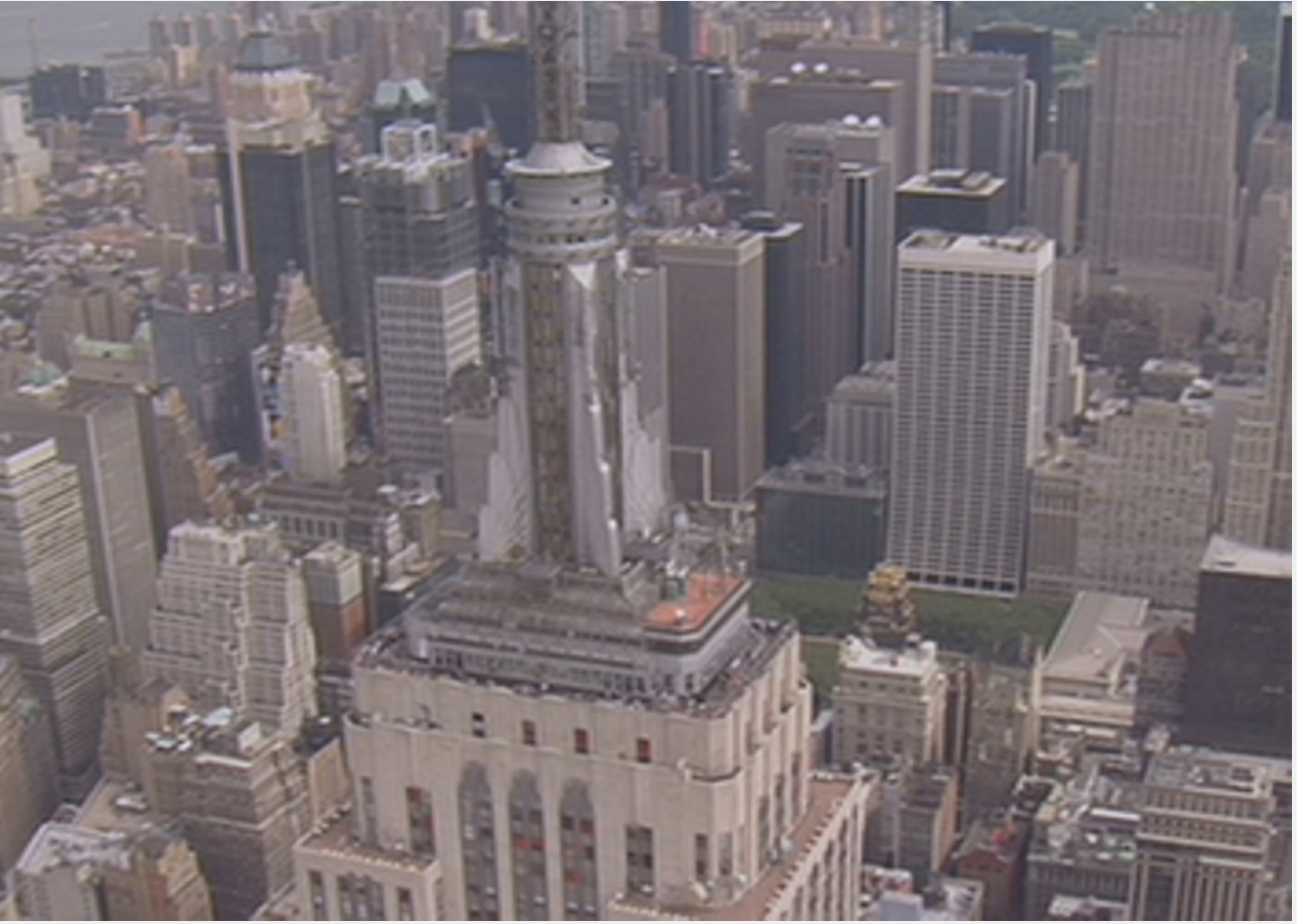
In color video completion we benchmark FBCP, ALS, TMac, TMac-TT and TMac-Square against two videos, New York City (NYC) and bus22 2 Videos available at https://engineering.purdue.edu/~reibman/ece634/. The other methods are computationally intractable or not applicable for in this experiment. For each video, the following preprocessing is performed: Resize the video to a tensor of size (). The first frame of each video can be seen in Figs. 8a and 8b. The mode is merged with the mode to form a third-order tensor, which we define here as a video sequence tensor (VST), of size (). Examples of the VST can be seen in the range 20000:20700 for in Figs. 8c and 8d. Hence, rather than performing an image completion on each frame, we perform our tensor completion benchmark on the entire video. It is important to highlight that we only benchmark with a ket augmented (not the third-order) VST due to computational intractability for high-dimensional low-order tensors.


Using KA, reshape the VST to a low-dimensional high-order tensor of size . The eleventh-order VST is directly used for the tensor completion algorithms.
| Algorithm | RSE | SSIM | RSE | SSIM | RSE | SSIM |
|---|---|---|---|---|---|---|
| FBCP | 0.210 | 0.395 | 0.210 | 0395 | 0.210 | 0.396 |
| ALS | 0.193 | 0.397 | 0.189 | 0.398 | 0.168 | 0.429 |
| TMac | 0.185 | 0.605 | 0.143 | 0.750 | 0.055 | 0.967 |
| TMac-TT | 0.072 | 0.876 | 0.066 | 0.902 | 0.053 | 0.949 |
| TMac-Square | 0.111 | 0.722 | 0.076 | 0.901 | 0.056 | 0.946 |
For the case of 95% missing entries, results of the benchmark can be seen in Figs. 11 and 12. The NYC results in Fig. 11 shows that FBCP and ALS are completely incomprehensible, whereas only the TMac-based algorithms can successfully complete the video. Moreover, in this case, TMac-TT outperforms all algorithms, which can be seen with the and mean structural similarity index () [48] (over all 81 frames) in Table II for . For the bus results in Fig. 12, TMac-TT outperforms all algorithms. The other TT rank-based algorithm ALS can only manage a simple structure of the bus, and FBCP cannot produce any resemblence to the original video. Table III summarizes the and mean results. With 90% missing entries, the results are similar to those of 95% missing entries, however, TMac-TT and TMac-Square are now comparable in performance for the NYC video. For the NYC video with , Table II shows that all TMac-based algorithms are comparable, with FBCP and ALS unable to reproduce a sufficient approximation. In the bus video, TMac-TT and TMac-Square provide comparable RSE and SSIM.
| Algorithm | RSE | SSIM | RSE | SSIM | RSE | SSIM |
|---|---|---|---|---|---|---|
| FBCP | 0.527 | 0.269 | 0.527 | 0.269 | 0.504 | 0.271 |
| ALS | 0.447 | 0.323 | 0.342 | 0.387 | 0.271 | 0.513 |
| TMac | 0.518 | 0.316 | 0.496 | 0.374 | 0.402 | 0.598 |
| TMac-TT | 0.154 | 0.807 | 0.092 | 0.932 | 0.062 | 0.974 |
| TMac-Square | 0.267 | 0.582 | 0.196 | 0.781 | 0.077 | 0.968 |
In summary, the bus video includes more vibrant colours and textures compared to the NYC video, which can be clearly seen from the overall performance in Tables II and III. It is important to highlight that TMac-TT still provides a high quality () approximation for the high missing ratio () test, where the next best result of TMac-Square had only . This demonstrates the superiority of using TMac-TT over the other algorithms for high missing ratio video completion problems.
VII Conclusion
A novel approach to the LRTC problem based on TT rank was introduced along with corresponding algorithms for its solution. The SiLRTC-TT algorithm was defined to minimize the TT rank of a tensor by TT nuclear norm optimization. Meanwhile, TMac-TT was proposed, which is based on the multilinear matrix factorization model to minimize the TT-rank. The latter is more computationally efficient due to the fact that it does not need the SVD. The proposed algorithms are employed to simulate both synthetic and real world data represented by higher-order tensors. For synthetic data, our algorithms prevails against the others when the tensors have low TT rank. Their performance is comparable in the case of low Tucker rank tensors. The TT-based algorithms are quite promising and reliable when applied to real world data. To validate this, we studied image and video completion problems. Benchmark results show that when applied to original tensors without tensor augmentation, our algorithms are comparable to STDC in image completion. However, in the case of augmented tensors, our proposed algorithms not only outperform the others, but also provide better recovery results when compared to the case without tensor order augmentation in both image and video completion experiments.
Applications of the proposed TT rank optimization based tensor completion to data compression, text mining, image classification and video indexing are under our interest.
References
- [1] T. G. Kolda and B. W. Bader, “Tensor decompositions and applications,” SIAM Review, vol. 51, no. 3, pp. 455–500, 2009.
- [2] M. Vasilescu and D. Terzopoulos, “Multilinear subspace analysis of image ensembles,” in Proc. IEEE Conf. Computer Vision and Pattern Recognition, vol. 2, June 2003, pp. 93–99.
- [3] J.-T. Sun, H.-J. Zeng, H. Liu, Y. Lu, and Z. Chen, “Cubesvd: A novel approach to personalized web search,” in Proc. 14th Int’l World Wide Web Conf. (WWW ’, 05), 2005, pp. 382–390.
- [4] T. Franz, A. Schultz, S. Sizov, and S. Staab, “Triplerank: Ranking semantic web data by tensor decomposition,” in The Semantic Web - ISWC 2009. Springer Berlin Heidelberg, 2009, vol. 5823, pp. 213–228.
- [5] J. Carroll and J.-J. Chang, “Analysis of individual differences in multidimensional scaling via an n-way generalization of “Eckart-Young” decomposition,” Psychometrika, vol. 35, no. 3, pp. 283–319, 1970.
- [6] R. A. Harshman, “Foundations of the PARAFAC procedure: Models and conditions for an “explanatory” multi-modal factor analysis,” UCLA Working Papers in Phonetics, vol. 16, no. 1, p. 84, 1970.
- [7] L. R. Tucker, “Some mathematical notes on three-mode factor analysis,” Psychometrika, vol. 31, no. 3, pp. 279–311, Sep 1966.
- [8] I. V. Oseledets, “Tensor-train decomposition,” SIAM J. Sci. Comput., vol. 33, no. 5, pp. 2295–2317, Jan 2011.
- [9] M. Fannes, B. Nachtergaele, and R. Werner, “Finitely correlated states on quantum spin chains,” Comm. Math. Phys., vol. 144, no. 3, pp. 443–490, 1992.
- [10] A. Klümper, A. Schadschneider, and J. Zittartz, “Matrix product ground states for one-dimensional spin-1 quantum antiferromagnets,” EPL, vol. 24, no. 4, p. 293, 1993.
- [11] D. Perez-Garcia, F. Verstraete, M. M. Wolf, and J. I. Cirac, “Matrix product state representations,” Quant. Info. Comput., vol. 7, no. 5, pp. 401–430, 2007.
- [12] J.-F. Cai, E. J. Candès, and Z. Shen, “A singular value thresholding algorithm for matrix completion,” SIAM J. Optim., vol. 20, no. 4, pp. 1956–1982, Jan 2010.
- [13] S. Ma, D. Goldfarb, and L. Chen, “Fixed point and Bregman iterative methods for matrix rank minimization,” Math. Programm., vol. 128, no. 1-2, pp. 321–353, Sep 2009.
- [14] B. Recht, M. Fazel, and P. A. Parrilo, “Guaranteed minimum-rank solutions of linear matrix equations via nuclear norm minimization,” SIAM Rev., vol. 52, no. 3, pp. 471–501, Jan 2010.
- [15] J. Liu, P. Musialski, P. Wonka, and J. Ye, “Tensor completion for estimating missing values in visual data,” IEEE Trans. Pattern Analysis and Machine Intelligence, vol. 35, no. 1, pp. 208–220, Jan 2013.
- [16] M. Signoretto, L. De Lathauwer, and J. A. K. Suykens†, “Nuclear norms for tensors and their use for convex multilinear estimation,” ESAT-SISTA, K. U. Leuven (Leuven, Belgium), Tech. Rep., 2010.
- [17] M. Signoretto, R. Van de Plas, B. De Moor, and J. Suykens, “Tensor versus matrix completion: A comparison with application to spectral data,” IEEE Signal Process. Lett., vol. 18, no. 7, pp. 403–406, Jul 2011.
- [18] S. Gandy, B. Recht, and I. Yamada, “Tensor completion and low-n-rank tensor recovery via convex optimization,” Inv. Probl., vol. 27, no. 2, p. 025010, Jan 2011.
- [19] T. Ryota, S. Taiji, K. Hayashi, and H. Kashima, “Statistical performance of convex tensor decomposition,” in Proc. Adv. Neural Inf. Process. Syst., Dec 2011, pp. 972–980.
- [20] H. Tan, B. Cheng, W. Wang, Y.-J. Zhang, and B. Ran, “Tensor completion via a multi-linear low-n-rank factorization model,” Neurocomputing, vol. 133, pp. 161–169, Jun 2014.
- [21] Y. Xu, R. Hao, W. Yin, and Z. Su, “Parallel matrix factorization for low-rank tensor completion,” IPI, vol. 9, no. 2, pp. 601–624, Mar 2015.
- [22] M. Bertalmio, G. Sapiro, V. Caselles, and C. Ballester, “Image inpainting,” in Proc. ACM Conf. Comp. Graph. (SIGGRAPH ’, 00), 2000, pp. 417–424.
- [23] N. Komodakis, “Image completion using global optimization,” in Proc. IEEE Comput. Vis. Pattern Recognit., vol. 1, 2006, pp. 442–452.
- [24] T. Korah and C. Rasmussen, “Spatiotemporal inpainting for recovering texture maps of occluded building facades,” IEEE Trans. Image Processing, vol. 16, no. 9, pp. 2262–2271, Sep 2007.
- [25] F. R. Bach, “Consistency of trace norm minimization,” J. Mach. Learn. Res., vol. 9, pp. 1019–1048, Jun 2008.
- [26] E. Candès and B. Recht, “Exact matrix completion via convex optimization,” Found. Comput. Math., vol. 9, no. 6, pp. 717–772, 2009.
- [27] G. Vidal, “Efficient classical simulation of slightly entangled quantum computations,” Phys. Rev. Lett., vol. 91, p. 147902, Oct 2003.
- [28] ——, “Efficient simulation of one-dimensional quantum many-body systems,” Phys. Rev. Lett., vol. 93, no. 4, Jul 2004.
- [29] I. V. Oseledets, E. E. Tyrtyshnikov, and N. L. Zamarashkin, “Tensor-train ranks of matrices and their inverses,” Comput. Meth. Appl. Math, vol. 11, no. 3, pp. 394–403, 2011.
- [30] E. Corona, A. Rahimian, and D. Zorin, “A tensor-train accelerated solver for integral equations in complex geometries,” arXiv, vol. abs/quant-ph/1511.06029, 2015.
- [31] I. V. Oseledets and S. V. Dolgov, “Solution of linear systems and matrix inversion in the tt-format,” SIAM Journal on Scientific Computing, vol. 34, no. 5, pp. A2718–A2739, 2012. [Online]. Available: http://dx.doi.org/10.1137/110833142
- [32] T. Mach, “Computing inner eigenvalues of matrices in tensor train matrix format,” in Proc. 9th European Conference on Numerical Mathematics and Advanced Applications, Leicester, 2011, pp. 781–788.
- [33] N. Lee and A. Cichocki, “Estimating a few extreme singular values and vectors for large-scale matrices in tensor train format,” SIAM Journal on Matrix Analysis and Applications, vol. 36, no. 3, pp. 994–1014, 2015.
- [34] S. Holtz, T. Rohwedder, and R. Schneider, “The alternating linear scheme for tensor optimization in the tensor train format,” SIAM J. Sci. Comput., vol. 34, no. 2, pp. A683–A713, Jan 2012.
- [35] L. Grasedyck, M. Kluge, and S. Kramer, “Variants of alternating least squares tensor completion in the tensor train format,” SIAM J. Sci. Comput., vol. 37, no. 5, pp. A2424–A2450, Jan 2015.
- [36] C. D. Silva and F. J. Herrmann, “Optimization on the hierarchical tucker manifold – applications to tensor completion,” Linear Algebra Appl., vol. 481, pp. 131–173, Sep 2015.
- [37] H. Rauhut, R. Schneider, and Z. Stojanac, “Tensor completion in hierarchical tensor representations,” in Compressed Sensing Appl. Springer, 2015, pp. 419–450.
- [38] J. A. Bengua, H. N. Phien, and H. D. Tuan, “Optimal feature extraction and classification of tensors via matrix product state decomposition,” in 2015 IEEE International Congress on Big Data, June 2015, pp. 669–672.
- [39] M. A. Nielsen and I. L. Chuang, Quantum Computation and Quantum Information. Cambridge University Press (CUP), 2009.
- [40] M. Fazel, “Matrix rank minimization with applications,” Ph.D. dissertation, PhD thesis, Stanford University, 2002.
- [41] M. Kurucz, A. A. Benczur, and K. Csalogany, “Methods for large scale SVD with missing values,” in Proc. 13th ACM SIGKDD Int. Conf. Knowl. Discov. Data Mining, 2007.
- [42] C. H. Bennett, D. P. DiVincenzo, J. A. Smolin, and W. K. Wootters, “Mixed-state entanglement and quantum error correction,” Phys. Rev. A, vol. 54, no. 5, pp. 3824–3851, Nov 1996.
- [43] C. Mu, B. Huang, J. Wright, and D. Goldfarb, “Square deal: Lower bounds and improved relaxations for tensor recovery,” in Proc. 31th Int’l Conf. Machine Learning, ICML 2014, vol. 32, 2014, pp. 73–81.
- [44] Z. Wen, W. Yin, and Y. Zhang, “Solving a low-rank factorization model for matrix completion by a nonlinear successive over-relaxation algorithm,” Math. Programm. Comput., vol. 4, no. 4, pp. 333–361, Jul 2012.
- [45] J. I. Latorre, “Image compression and entanglement,” arxiv, vol. abs/quant-ph/0510031, 2005.
- [46] Q. Zhao, L. Zhang, and A. Cichocki, “Bayesian cp factorization of incomplete tensors with automatic rank determination,” IEEE Transactions on Pattern Analysis and Machine Intelligence, vol. 37, no. 9, pp. 1751–1763, Sept 2015.
- [47] Y. L. Chen, C. T. Hsu, and H. Y. M. Liao, “Simultaneous tensor decomposition and completion using factor priors,” IEEE Transactions on Pattern Analysis and Machine Intelligence, vol. 36, no. 3, pp. 577–591, March 2014.
- [48] Z. Wang, A. C. Bovik, H. R. Sheikh, and E. P. Simoncelli, “Image quality assessment: from error visibility to structural similarity,” IEEE Transactions on Image Processing, vol. 13, no. 4, pp. 600–612, April 2004.