{CCSXML}

¡ccs2012¿ ¡concept¿ ¡concept_id¿10003752.10010070.10010099.10010101¡/concept_id¿ ¡concept_desc¿Theory of computation Algorithmic mechanism design¡/concept_desc¿ ¡concept_significance¿500¡/concept_significance¿ ¡/concept¿ ¡concept¿ ¡concept_id¿10003752.10010070.10010099.10010107¡/concept_id¿ ¡concept_desc¿Theory of computation Computational pricing and auctions¡/concept_desc¿ ¡concept_significance¿500¡/concept_significance¿ ¡/concept¿ ¡concept¿ ¡concept_id¿10003752.10003809.10003636.10003813¡/concept_id¿ ¡concept_desc¿Theory of computation Rounding techniques¡/concept_desc¿ ¡concept_significance¿100¡/concept_significance¿ ¡/concept¿ ¡/ccs2012¿

\ccsdesc

[500]Theory of computation Algorithmic mechanism design \ccsdesc[500]Theory of computation Computational pricing and auctions \ccsdesc[100]Theory of computation Rounding techniques

{bottomstuff}

This work is supported by the National Science Foundation under grant AST-1343381 and the SURE (Summer Undergraduate Research Experience) program at the University of Michigan. The authors would like to thank Rakesh Vohra and Thanh Nguyen for comments on an earlier draft.

Author’s addresses: D. Tang and V. G. Subramanian, Electrical Engineering and Computer Science Department, University of Michigan; email: {dwtang,vgsubram}@umich.edu.

Approximately Envy-Free Spectrum Allocation with Complementarities

DOI: XXXXXXX.XXXXXXX

Dengwang Tang Vijay Subramanian Affiliation: University of Michigan Affiliation: University of Michigan

Abstract

With spectrum auctions as our prime motivation, in this paper we analyze combinatorial auctions where agents’ valuations exhibit complementarities. Assuming that the agents only value bundles of size at most $k$ and also assuming that we can assess prices, we present a mechanism that is efficient, approximately envy-free, asymptotically strategy-proof and that has polynomial-time complexity. Modifying an iterative rounding procedure from assignment problems, we use the primal and dual optimal solutions to the linear programming relaxation of the auction problem to construct a lottery for the allocations and to assess the prices to bundles. The allocations in the lottery over-allocate goods by at most $k-1$ units, and the dual prices are shown to be (approximately) envy-free irrespective of the allocation chosen. We conclude with a detailed numerical investigation of a specific spectrum allocation problem.

keywords

Combinatorial auctions, Complementaries, Supporting prices, Walrasian prices, Envy-free pricing mechanism

1 Introduction

Market design is widely applied to many real-world problems that have interesting underlying resource allocation questions [24, 17, 15]. Most of the problems involve allocation of indivisible goods where the preference exhibit complementarities with preferences over bundles of goods, and also externalities. Some of these problems, such as matching of residents to hospitals, matching of students to schools, or kidney exchanges, either explicitly bar the use of monetary transfers or prices to facilitate market-making, or cannot use prices owing to non-numeraire preferences. In many others problems, such as online sponsored search auctions, market clearing in electricity markets, or spectrum auctions, bids and prices obtained via combinatorial auctions [10, 5, 17] are the mainstay of the underlying market-making. Despite the wide-applicability of combinatorial auctions in the latter class of problems, it is well-understood that without any restrictions on the agent utilities, the problems are computationally intractable. In this paper, we focus on the generic combinatorial auction problem, and under specific restrictions on the agent utilities present a randomized mechanism with polynomial-time complexity that ensures ex-post approximate envy-freeness and asymptotic strategy-proofness.

Our main motivation for this work is spectrum auctions and markets [4, 18, 6, 7, 8]. Owing to interference considerations, it is easily seen that agents (service providers) obtain higher total utilities for allocations when bands are adjacent either in frequency or space as opposed to when the bands are separately allocated. Given the increased demand and utilization of the airwaves, many governments have successfully conducted auctions to license spectrum bands for use by commercial service providers, and sometimes via open-access. As many more auctions are expected in the future, understanding classes of utilities for which there exist optimal or almost optimal mechanisms with polynomial-time complexity is an important area of research.

One of the principal reasons for the intractability of the combinatorial auction problem is that it includes the knapsack problem with the additional complexity of having an exponential (in the number of goods being auctioned) number of integer variables. In addition, even the linear programming relaxation is a hard problem as the number of variables is still exponential in the number of goods. There is considerable research on polynomial-time approximation algorithms in this context [22, 30, 3, 5, 19, 13, 12, 23]. Starting with the assumption of a single-minded¹¹ 1 Different agents are identified via specific bundles, say $S_{i}$ for agent $i$ , and they have a positive constant utility only for all bundles that contain $S_{i}$ . buyer, the authors in [5] present a greedy, constant-factor, polynomial-time, and strategy-proof approximation mechanism for this problem that solicits bids and determines prices for the agents who get allocated bundles. This approximation mechanism is then generalized to larger class of utilities that can be obtained from the single-minded buyer setting using elementary operations. While this scheme provides a mechanism with many good properties, it is not guaranteed to be efficient. With the same family of utilities, if the linear-programming relaxation yields an integer solution [5], then the Second Welfare Theorem insists that the dual variables can be used to determine Walrasian market clearing prices [2, 5, 27] to be the assessed to agents that get allocated bundles; the linear programming relaxation can be solved in polynomial-time with the family of utilities considered. Complementary slackness also obtains envy-freeness [5, 27], wherein no agent gets a higher return for the allocation of any other agent, and hence doesn’t envy it. Furthermore, it is easily shown that in the presence of many agents, no agent gains much by being untruthful about their valuations, i.e., asymptotic strategy-proofness also obtains. These results will be important precedents that will be one part of the related work.

Some recent developments for matching and assignment problems with complementarities, where either the valuations are non-numeraire or where prices cannot be assessed, are also important precedents for our work. In [20] and [21] the authors consider one-sided and two-sided matchings with complementarities. An important restrictions on the utilities that they impose is to assert that agents do not value bundles of size (number of good in the bundle include multiplicities) greater than $k$ (a parameter); just as in the single-minded buyer setting, the valuation of the larger bundles can equivalently be set to the maximum of the bundles contained within. The mechanisms developed then solve the linear programming relaxation with envy-freeness explicitly accounted for as a constraint (because prices cannot assessed in such problems). The key innovation is to then present a polynomial-time integer-rounding-based lottery procedure such that the linear programming optimal solution is in the convex-hull of the integer solutions with the added property that none of the integer solutions exceed the supply constraints by more than $k-1$ units. Note that efficiency is guaranteed as the expected utility is exactly that obtained from the solution of the linear programming relaxation.

In this paper we adopt the $k$ -sized bundles restrictions on the utilities from [20] and [21], and ask whether there exists a polynomial-time efficient randomized mechanism when the valuations are numeraire, and agents have quasilinear utilities. The key difference in our problem is the ability to charge prices, and so we further look for a mechanism that a’la Walrasian prices naturally obtain envy-freeness, instead of imposing it as a constraint in the linear programming relaxation. As mentioned earlier, spectrum auctions are one of the main motivations for us to study such mechanisms, and there are policy guidelines that are being discussed for the upcoming incentive auctions by the FCC where certain players like AT&T and Verizon will have restrictions on the bands that they can bid on [9, 26]. Our $k$ -bundle constraint on the utilities is a natural form of such restrictions.

Our mechanism for allocation, called the POPT (Priced OPT) mechanism, starts with the linear programming relaxation of the allocation problem with just the demand and supply constraints; we call this problem by LIP. We solve LIP via the simplex method to obtain an extreme point optimal and the corresponding Lagrange multipliers (dual optimal). We then modify the integer-rounding procedure in [20] such that each of the integer solutions is the optimal solution of a related linear programming problem such that the dual optima include the dual optima for LIP. This is an important modification that allows us to construct the prices for our mechanism. We believe that this idea can be used in contexts. We then follow the lottery construction procedure from [20] with a few small modifications. We prove the (approximate) envy-freeness of our mechanism first by showing a market-clearing property of our prices that we call as supporting the allocation, and then by using complementary slackness we demonstrate envy-freeness.

The paper is organized as follows. In Section 2 we describe the POPT mechanism and prove many properties of it, including approximate envy-freeness. We analyze the performance of the mechanism in Section 3. We then briefly describe the open-source implementation of the mechanism in Section 4 and conclude in Section 5.

2 Mechanism Setup

We start by describing the mechanism. Thereafter, we elaborate on each of the steps of the mechanism and prove properties of it.

For the POPT mechanism, we will use the following procedure to get an approximate efficient allocation of the goods.

POPT mechanism:

1.

Set up initial linear programming problem (LIP).
2.

Solve (LIP) and get solution $x^{*}$ .
3.

Perform Lottery Construction process on $x^{*}$ to get integral solutions
4.

Construct a lottery of the integral solutions that (approximately) has the expected solution being $x^{*}$ .
5.

Solve the dual of (LIP) to get POPT prices that support the allocation.

2.1 Initial Linear Programming Problem

We assume that we have a set $N$ of agents and set $G$ of good types. For every type $j$ of good, we have the supply for the good to be $s_{j}$ , where all goods of a given type are identical. A bundle is denoted by a vector $B\in\mathbb{Z}_{+}^{|G|}$ where the j-th coordinate $B_{j}$ denotes the number of good of type $j$ in bundle $B$ . If $B_{j}^{1}\leq B_{j}^{2}$ for all $j\in G$ and $B^{1}\neq B^{2}$ , we say that $B^{1}\prec B^{2}$ . Denote the set of all available bundles as $\mathcal{B}$ . Define the function $x_{i}:\mathcal{B}\mapsto\{0,1\},i\in N$ as the indicator variable for the allocation of bundle $B$ to agent $i$ . Therefore, $x_{i}(B)=1$ means that bundle $B$ is allocated to agent $i$ . Function $u_{i}:\mathcal{B}\mapsto\mathbb{R},i\in N$ determines the valuations of each agent for all possible bundles, i.e. $u_{i}(B)=p$ means that bundle $B$ has value $p$ for agent $i$ .

To make this problem solvable in polynomial time, we assume that the agents are only interested in bundles with size less than or equal to $k$ . In other words, the valuation can only be positive for bundles $B$ such that

\sum_{j\in G}B_{j}\leq k~~~~~~\forall B\in\mathcal{B}.

Therefore, for bundles $B$ with size larger than $k$ we fix $x_{i}(B)=0$ ; alternatively we can follow the convention for single-mind buyers and set the valuations of a bundle with size greater than $k$ to be the maximum of the valuation of its subsets. In either case, then we can reduce the set $\mathcal{B}$ to contain only the k-bundles, which denotes the bundles with size less than or equal to $k$ . Furthermore, we relax $x_{i}(B)$ to take values in $[0,1]$ . This way the problem of solving $x_{i}(B)$ can be formulated as a linear programming problem on a convex set.

The demand constraints for the allocation insist that every agent gets at most one bundle. These are given by

\displaystyle\sum_{B\in\mathcal{B}}x_{i}(B)\leq 1~~~~~~\forall i\in N.

(Demand)

The supply constraints ensure that the goods are not over-allocated. They are given by

\displaystyle\sum_{i\in N}\sum_{B\in\mathcal{B}}B_{j}x_{i}(B)\leq s_{j}~~~~~~\forall j\in G.

(Supply)

The objective function to be maximized is the total utility of the agents. Therefore the initial linear programming problem can be formulated as

\displaystyle\begin{array}[]{ccll}&\displaystyle\max_{x\geq 0}&\displaystyle\sum_{i\in N}\sum_{B\in\mathcal{B}}u_{i}(B)x_{i}(B)&\\ &\mathrm{s.t.}&\displaystyle\sum_{B\in\mathcal{B}}x_{i}(B)\leq 1&\forall i\in N,\\ &&\displaystyle\sum_{i\in N}\sum_{B\in\mathcal{B}}B_{j}x_{i}(B)\leq s_{j}&\forall j\in G.\end{array}

We make some modifications to the coefficients of the problem, and we get

\displaystyle\begin{array}[]{ccll}&\displaystyle\max_{x\geq 0}&\displaystyle\sum_{i\in N}\sum_{B\in\mathcal{B}}w_{i}(B)u_{i}(B)x_{i}(B)&\\ &\mathrm{s.t.}&\displaystyle\sum_{B\in\mathcal{B}}x_{i}(B)\leq 1&\forall i\in N,\\ &&\displaystyle\sum_{i\in N}\sum_{B\in\mathcal{B}}B_{j}x_{i}(B)\leq\tilde{s}_{j}:=s_{j}-\epsilon_{j}&\forall j\in G.\end{array}

(LIP)

where $w_{i}(B)$ are weights which typically takes values near 1 and $\epsilon_{j}\ll 1$ are modification variables. For our mechanism, we choose $w_{i}$ and $\epsilon_{j}$ randomly, where $w_{i}(B)$ are drawn i.i.d. uniformly on $[1-\delta_{w},1+\delta_{w}]$ , and $\epsilon_{j}$ are drawn i.i.d. uniformly on $[\delta_{\epsilon},2\delta_{\epsilon}]$ . Here $\delta_{w}\ll 1$ and $\delta_{\epsilon}\ll 1$ are preset values. The reason for this is to ensure asymptotic strategy-proofness, and this will be discussed in the Section 3.

To solve the problem, we first solve (LIP) and get a solution $x^{*}$ , which is most likely to be fractional. If it is fractional, we run the lottery construction process using the solution $x^{*}$ to get a few integral solutions to form a lottery to determine the resulting allocation.

2.2 Obtaining Integral Solutions

For the lottery construction we need a subroutine called Iterative Rounding (IR). Given any reward vector $c$ , the Iterative Rounding procedure basically takes any point $z$ which satisfies (Demand) and (Supply) as input, and outputs an integral $\overline{x}$ . This procedure can be denoted as a function $\overline{x}=\mathrm{IR}(z)$ or $\overline{x}=\mathrm{IR}(z;c)$ .

2.2.1 Iterative Rounding

For the Iterative Rounding procedure, we basically follow the procedure described in [20] but we also make some modifications. For any reward vector $c\in\mathbb{R}^{|N|\times|\mathcal{B}|}$ which has the same size as the input $z$ , the procedure is as described in Algorithm 1.

ALGORITHM 1 Iterative Rounding

Input: A point

z

which satisfies (Demand) and (Supply)

Output: An integral point

z^{(\tau)}

which satisfies (Demand) and (Supply+k-1)

G^{(0)}=G,~\mathcal{B}_{i}^{(0)}=\mathcal{B}~~~\forall i\in N,~\tilde{s}_{j}^{(0)}=\tilde{s}_{j}~~~\forall j\in G,~z^{(\tau)}=z,\tau=0

;

N^{(\tau)}=\{i\in N:\sum_{i\in N}z_{i}(B)=1\}

;

repeat

z^{(\tau)}

is integral then

break

end if some but not all of

z^{(\tau)}_{i}(B)

are integral then

\mathcal{B}_{i}^{(\tau+1)}=\{B\in\mathcal{B}:0<z_{i}^{(\tau)}(B)<1\}

;

\tilde{s}_{j}^{(\tau+1)}=s_{j}^{\prime(\tau)}-\sum_{i\in N}\sum_{B\in\mathcal{B}_{i}^{(\tau)}\backslash\mathcal{B}_{i}^{(\tau+1)}}B_{j}z_{i}^{(\tau)}(B)~~~~~~\forall j\in G^{(\tau)}.

;

The updated linear programming problem is then

\displaystyle\begin{array}[]{ccll}&\displaystyle\max_{x\geq 0}&\displaystyle\sum_{i\in N}\sum_{B\in\mathcal{B}^{(\tau+1)}_{i}}c_{i}(B)x_{i}(B)&\\ &\mathrm{s.t.}&x_{i}(B)=z_{i}^{(\tau)}(B)&\forall i\in N,B\in\mathcal{B}\backslash\mathcal{B}_{i}^{(\tau+1)}\\ &&\displaystyle\sum_{B\in\mathcal{B}^{(\tau+1)}_{i}}x_{i}(B)=1&\forall i\in N^{(\tau)},\\ &&\displaystyle\sum_{B\in\mathcal{B}^{(\tau+1)}_{i}}x_{i}(B)\leq 1&\forall i\in N\backslash N^{(\tau)},\\ &&\displaystyle\sum_{i\in N}\sum_{B\in\mathcal{B}^{(\tau+1)}_{i}}B_{j}x_{i}(B)\leq\tilde{s}_{j}^{(\tau+1)}&\forall j\in G^{(\tau)}.\end{array}

(ULIP)

Solve (ULIP) to get an extreme point solution

z^{*}

, set

z^{(\tau+1)}=z^{*}

;

end if none of

z_{i}^{(\tau+1)}(B)

is integral then

G^{(\tau+1)}=\{j\in G^{(\tau)}:\sum_{i\in N}\sum_{B\in\mathcal{B}_{i}^{(\tau+1)}}B_{j}>\lceil\tilde{s}^{(\tau+1)}_{j}\rceil+k-1\}

;

Comment: By [20] there must exist some

j\in G^{(\tau)}

such that

\sum_{i\in N}\sum_{B\in\mathcal{B}_{i}^{(\tau+1)}}B_{j}\leq\lceil\tilde{s}^{(\tau+1)}_{j}\rceil+k-1.

end

\tau=\tau+1

until Forever;

The main difference between our proposed iterative rounding procedure and that in [20] lies in the second step where we set $N^{(\tau)}$ . In our procedure, we preserve the equality constraints so that we can ensure that the set of active demand constraints for input $z$ is a subset of that of output $z^{(\tau)}$ . Therefore we can ensure that the Lagrange multipliers of the original problem (LIP) also apply to $z^{\tau}$ . This will be discussed further in Theorem 2.3 in Section 2.3. It then promotes the existence of supporting prices for the allocation scheme $z^{(\tau)}$ , which would be discussed in Theorem 2.6.

It is easy to see that the procedure would finish in polynomial time, since in each iteration, either at least one variable is eliminated or at least one constraint is eliminated. So the number of rounds cannot be larger than sum of the number of constraints and the number of variables.

Define the approximate supply constraint

\displaystyle\sum_{i\in N}\sum_{B\in\mathcal{B}}B_{j}x_{i}(B)\leq s_{j}+k-1~~~~~~\forall j\in G.

(Supply+k-1)

We have the following results.

Theorem 2.1.

For any reward vector $c$ and any vector $z$ that satisfies (Supply), we have $\overline{z}=\mathrm{IR}(z;c)$ to satisfy (Supply+k-1) and $c^{T}\overline{z}\geq c^{T}z$ .

Proof 2.2.

See Appendix B in [20].

From Theorem 2.1, we know that for any $z$ that satisfies (Demand) and (Supply) and any vector $c$ , we can always find out an integral $\overline{z}$ (using Iterative Rounding Algorithm) which satisfies (Demand) and (Supply+k-1) such that $c^{T}\overline{z}\geq c^{T}z$ .

2.3 Lottery Construction

For the Lottery Construction part, we also basically follow the algorithm described by [20], but here again we make some modifications.

The procedure is as described in Algorithm 2.

ALGORITHM 2 Lottery Construction

Input: Fractional Optimal Solution

x^{*}

Output: Set

F

of integral points that satisfy (Demand) and (Supply+

k

-1).

c_{i}^{(1)}(B)=w_{i}(B)u_{i}(B),\forall B\in\mathcal{B}

;

x^{\prime}=\mathrm{IR}(x^{*};c^{(1)})

;

c_{i}^{(2)}(B)=-w_{i}(B)u_{i}(B),\forall B\in\mathcal{B}

;

x^{\prime}=\mathrm{IR}(x^{*};c^{(2)})

;

F^{(0)}=\{x^{\prime},x^{\prime\prime}\}

\tau=0

;

\varepsilon

is a preset allowable error;

\delta_{z}=\dfrac{\delta_{\epsilon}}{\sqrt{|N|\sum_{B\in\mathcal{B}}B_{j}^{2}}}

for some

j\in G

;

Comment: Note that the value of

\delta_{z}

is independent of

j

, since

\mathcal{B}

is the set of all

k

-bundles and it is symmetric with regard to any

j\in G

repeat

y^{*}=\arg\min_{y}\{\|y-x^{*}\|:

y

lies in the convex hull

E

of all points in

F^{(\tau)}\}

;

(Quadratic Programming)

\|y^{*}-x^{*}\|<\varepsilon

then

break

else

(

y^{*}

may lie on a surface of the convex hull

E

. There exist a minimal subset

F^{\prime}\subseteq F^{(\tau)}

such that

y\in\mathrm{int}E^{\prime}

where

E^{\prime}

is the convex hull of

F^{\prime}

F^{(\tau+1)}=F^{\prime}

;

z=x^{*}+\delta_{z}\frac{x^{*}-y^{*}}{\|x^{*}-y^{*}\|}

\overline{z}=\mathrm{IR}(z,x^{*}-y^{*})

;

F^{(\tau+1)}=F^{(\tau+1)}\cup\{\overline{z}\}

;

end

\tau=\tau+1

until Forever;

The main difference between our proposed procedure and that of [20] lies in the initialization steps. In the two steps we initialize a non-empty set $F^{(0)}$ so that the quadratic programming problem in the first step in the loop would always have a solution.

The authors of [20] proved that the above algorithm terminates in polynomial time. After the algorithm terminates, we get a the set of (integral) points $F$ , where the fractional solution $x^{*}$ of (LIP) is contained in the convex hull of all points in $F=\{x^{1},x^{2},\cdots,x^{l}\}$ . The coefficients $\lambda_{i}$ where $x^{*}=\sum_{i=1}^{l}\lambda_{i}x^{i},~\sum_{i=1}^{l}\lambda_{i}=1$ is also calculated from the quadratic programming problem in the loop. Then we can randomly select one vector $x^{i}$ from set $F$ (with probability $\lambda_{i}$ ) as the final allocation.

Theorem 2.3.

Suppose $x^{*}$ is a solution for (LIP). Any $\overline{x}\in F$ is an optimal solution to the following problem.

\displaystyle\begin{array}[]{ccll}&\displaystyle\max_{x\geq 0}&\displaystyle\sum_{i\in N}\sum_{B\in\mathcal{B}}w_{i}(B)u_{i}(B)x_{i}(B)&\\ &\mathrm{s.t.}&\displaystyle\sum_{B\in\mathcal{B}}x_{i}(B)\leq 1&\forall i\in N,\\ &&\displaystyle\sum_{i\in N}\sum_{B\in\mathcal{B}}B_{j}x_{i}(B)\leq\overline{s}_{j}&\forall j\in G,\end{array}

(MLIP)

where

\displaystyle\overline{s}_{j}:=\begin{cases}\tilde{s}_{j}&\displaystyle\sum_{i\in N}\sum_{B\in\mathcal{B}}B_{j}x^{*}_{i}(B)<\tilde{s}_{j}~\mathrm{and}~\displaystyle\sum_{i\in N}\sum_{B\in\mathcal{B}}B_{j}\overline{x}_{i}(B)\leq\tilde{s}_{j}\\ \displaystyle\sum_{i\in N}\sum_{B\in\mathcal{B}}B_{j}\overline{x}_{i}(B)&\mathrm{otherwise}\end{cases}

for all $j\in G$ , and we have $\overline{s}_{j}\leq s_{j}+k-1$ for all $j\in G$ . Furthermore, any dual solution of (LIP) is also a dual solution of (MLIP).

Proof 2.4.

See Appendix A.∎

From Theorem 2.3 we see that if we modify the supply vector from $\tilde{s}_{j}$ to $\overline{s}_{j}$ , then we have the allocation linear programming problem to have an integral optimal solution. The optimality of the solution for a specified problem ensures that the Lagrange multiplier associated with the original problem (LIP) is also a Lagrange multiplier for (MLIP). This is important in establishing the existence of supporting prices, which will be discussed further in Theorem 2.6. Furthermore, the fact that $\overline{s}_{j}\leq s_{j}+k-1$ indicates that for any final allocation scheme, we need no more than $k-1$ additional goods for each type of good to fulfill the allocation just as in [20].

2.4 POPT Prices

In this section, we will construct a set of prices from the dual solution of (MLIP) in Theorem 2.3. Then we will discover some nice properties of the prices. We will prove that the prices support the allocation scheme and are envy-free. We will call these prices POPT prices.

2.4.1 Dual Solution as Supporting Prices

After getting the allocation from the above procedure, we would like to find a set of prices for different kind of goods to support the allocation. We would like the prices to have the property that every agent chooses the bundle that yields the best (within some acceptable error) payoff, resulting in the designed allocation.

Definition 2.5.

Let $\epsilon_{u}$ be the acceptable error²² 2 For example, when people make trades of millions of dollars, they would not care the utility difference of only one dollar. In this case $\epsilon_{u}=1$ dollar. In general $\epsilon_{u}$ can be set arbitrarily small. in utility, and $P(B)$ denote the price of bundle $B$ , then a set of prices is said to support allocation scheme $\overline{x}$ if for every agent, either the agent chooses some bundle $\hat{B}$ according to $\overline{x}$ and

\displaystyle u_{i}(\hat{B})-P(\hat{B})\geq u_{i}(B)-P(B)-\epsilon_{u},~~~\forall B\in\mathcal{B},

or he chooses to buy nothing and

\displaystyle u_{i}(B)-P(B)\leq\epsilon_{u},~~~\forall B\in\mathcal{B}.

If $\epsilon_{u}=0$ , then the definition coincides with users with allocations in their preferred set of bundles (after accounting for the price), and users with no allocations making a non-positive return on every good. Market-clearing prices have this property along with the market-clearing property.

Theorem 2.6.

The set of supporting prices associated with any designed allocation $\overline{x}\in F$ (from lottery construction procedure of POPT mechanism) exists.

Proof 2.7.

See Appendix B.

Remark 2.8.

From Theorem 2.6, we know that supporting prices always exists for the allocation we get from Lottery Construction procedure, since the solution of dual of (MLIP) are supporting prices. From the proof of the Theorem 2.3 (in Appendix A), we can see that the Lagrange multipliers of original (LIP) are also multipliers of (MLIP), which means that a dual solution of (LIP) is also a dual solution of (MLIP). Therefore a dual solution of (LIP) forms a supporting price for any designed allocation scheme $\overline{x}\in F$ . Ensuring that this property holds is an important contribution of our paper.

2.4.2 Dual Solution as Approximately Envy-free Prices

The following part shows that under the prices given by the dual solution of (MLIP), the allocation suggested by $\overline{x}$ is approximately envy-free. We first give a formal definition of envy-freeness, then we show the allocation and prices we obtain ensure this property. It is important to note that unlike in [20], envy-freeness is not added as an explicit constraint in (LIP).

Definition 2.9.

Let $P(B)$ denote the price of bundle $B$ (the price of an empty bundle is 0), $x$ be the allocation vector, and $\epsilon_{u}$ be the acceptable error. Then the pricing rule is said to be approximately envy-free if³³ 3 The definition is an extension of the definition in [16] as they consider exact envy-freeness, i.e. the case when $\epsilon_{u}=0$ .

\displaystyle\sum_{B\in\mathcal{B}}[u_{i}(B)-P(B)]x_{i}(B)\geq\sum_{B\in\mathcal{B}}[u_{i}(B)-P(B)]x_{k}(B)+\epsilon_{u},~~~\forall i,k\in N

Theorem 2.10.

Under any optimal allocation $x^{*}$ for problem (LIP), if the pricing rule is

\displaystyle P(B)=\sum_{j\in G}B_{j}p_{j}^{*}

where $p_{j}^{*}~(j\in G)$ is some Lagrange multiplier associated with supply constraints of (LIP), then the approximate envy-freeness condition holds.

Proof 2.11.

See Appendix C.

Proposition 2.12.

For any integral allocation $\overline{x}\in B$ , if the price rule is

\displaystyle P(B)=\sum_{j\in G}B_{j}p_{j}^{*}

where $p_{j}^{*}~(j\in G)$ is some Lagrange multiplier associated with supply constraints of (LIP), then the approximate envy-freeness condition (not only holds for $x^{*}$ but) also holds for $\overline{x}$ .

Proof 2.13.

From the Proof of Theorem 2.3 (Appendix A) we know that if $(\pi^{*},v^{*})$ is a set of Lagrange multiplier of (LIP), then $(\pi^{*},v^{*})$ is also a set of Lagrange multiplier of (MLIP). Since $\overline{x}$ is a solution to (MLIP) according to Theorem 2.3, we have $p^{*}_{j}$ to be also the Largrange Multipliers for (MLIP). Apply Theorem 2.6 to (MLIP) then we would find that the approximate envy-freeness condition holds for $\overline{x}$ .

From Proposition 2.12 we know that we can calculate the dual solution of (LIP) instead of (MLIP) to figure out a set of POPT prices that supports all possible allocation $\overline{x}$ . This is important, as we can then get the dual solution of (LIP) through the process of solving (LIP). We do not need to construct and solve the dual of (MLIP), which makes the calculation of prices much more efficient.

2.5 Summary of POPT Mechanism

For the POPT mechanism, we try to find an approximately efficient and envy-free allocation scheme for spectrum band allocation with complementarities as well as the price of goods associated with the scheme. To achieve this we first relax the constraint to allow the allocation indicator variables to be real-valued, and we set up an initial linear programming problem (LIP) with only the demand and supply constraints. We then solve (LIP) to get a solution $x^{*}$ .

Then, we perform the Lottery construction process on $x^{*}$ to round $x^{*}$ to a set $F$ of integral solutions. We then assign a probability to each of these integral solutions to form a lottery such that it has expectation $x^{*}$ .

When realizing the mechanism, we choose an integral solution in $F$ based on some random event (such as rolling a die) so that every integral solution has the probability of being chosen equal to the probability assigned to it.

We solve the dual problem of (LIP) at the same time to obtain the prices associated with POPT mechanism. As implied by Theorem 2.6 and Theorem 2.10, this price supports any allocation scheme given by POPT mechanism and it is approximately envy-free.

3 Analysis

In this section we start by showing asymptotic strategy-proofness of the POPT mechanism, and then present a numerical analysis of a specific spectrum allocation problem.

3.1 Theoretical Analysis

In this part, we will first analyze the complexity and strategy-proofness of the mechanism. Then we will discuss on the methods for solving the linear programming problems for the mechanism.

3.1.1 Complexity Analysis

Fix $k$ , the calculation of the approximate optimal allocation can be performed in polynomial time with regard to $|N|$ and $|G|$ . (See Appendix D) The mechanism is therefore much more computationally efficient than the optimal mechanism: integer linear programming with VCG prices.

3.1.2 Asymptotic Strategy-proofness

One important property that a mechanism should have is strategy-proofness. A mechanism is said to be strategy-proof if the best strategy for any individual agent is to report his or her utility truthfully.

Consider that we have finite types of agents, and the set of type is denoted as $\Theta=\{\theta_{1},\theta_{2},\cdots,\theta_{m}\}$ , and the number of agents with type $\theta$ is $n_{\theta}$ . Denote the utility of bundle $B$ for agent of type $\theta$ as $u_{\theta}(B)$ and the type of agent $i$ as $\beta_{i}$ . Following [20] we define asymptotic strategy-proofness as follows.

Definition 3.1.

If $\overline{x},\overline{p}$ are the allocation vector and price vector that POPT mechanism gives when every agent report his or her type $\beta_{i}$ truthfully, and $\tilde{x}$ and $\tilde{p}$ are the corresponding results when agent $i$ report as type $\gamma$ while others report their types truthfully, a mechanism is called asymptotically strategy-proof if for any $\varepsilon_{0}>0$ there exists $N_{0}\in\mathbb{N}$ such that when $n_{\theta}>N_{0}$ for all $t=1,2,\cdots,m$ we have

\displaystyle\mathbb{E}\left[\sum_{B\in\mathcal{B}}\left(u_{\beta_{i}}(B)-\overline{p}(B)\right)\overline{x}_{i}(B)\right]\geq\mathbb{E}\left[\sum_{B\in\mathcal{B}}(u_{\zeta}(B)-\tilde{p}(B))\tilde{x}_{i}(B)\right]-\epsilon_{u}-\varepsilon_{0}

for all $i\in N,\zeta\in\Theta$ , where $\epsilon_{u}>0$ is the acceptable error.

This definition generally means that when the number of agents comes large, the increase of average payoff that an agent could get by misreporting his or her type becomes less and less and converges to a number less than or equal to $\epsilon_{u}$ . If the agents are risk-neutral, then this implies that an agent would not have an impulse to mis-report her type.

The following theorem is a variant of Theorem 3.3 in [20]. The additional steps arise from ensuring the convergence of the dual variables.

Theorem 3.2.

Set $w_{i}$ to be the same for the same type of agents, then the mechanism POPT is asymptotically strategy-proof.

Proof 3.3.

See Appendix E.

Therefore, we can say that the POPT mechanism is approximately truthful. When the number of agents get large, one can get approximately the best payoff by reporting his or her true type.

3.1.3 Methods for Solving Linear Programming Problem

For the initial linear programming problem (LIP) and updated linear programming problems (ULIP) in Iterative Rounding, we choose the Simplex method to solve them. The reasons for us to choose Simplex method are given as follows.

1.

It is fast in practice. The average complexity of simplex method is $O(s)$ where $s$ is the number of constraints. In (LIP), we have significantly fewer constraints than variables, thus it is very suitable for (LIP).
2.

It solves the problem based on extreme points. In (LIP) and all (ULIP), we would like to find an extreme point solution. Simplex method ensures that the solution is an extreme point.

3.2 Empirical Analysis

In the following part, we will analyze the whole mechanism from multiple perspectives. Based on a utility model that is described in [28], we will first investigate the efficiency of the mechanism on a utility model. Then we will investigate how many more goods we need on average to fulfill the allocation suggested by the mechanism. We will use a grid structure for the analysis, so next we will discuss how the prices and the allocations change based on location. Finally, we finely categorize the form of integer solutions produced by our mechanism, especially the shapes of the bundles.

The utility model is constructed in the following way: Consider a 2-D area that is a $m_{g}\times n_{g}$ grid, each grid has unit area and it is considered as a type of good. For each grid (good) there are $s_{g}$ bands, which can be viewed as the available supply for the grid. There are $N_{a}$ agents and each agent would like at most a bundle of $k_{a}$ goods.

For each agent, there are some end-users distributed via a 2-D spatial Poisson process in the area, with parameter $\mu$ (person/unit area). The parameter $\mu$ determines the system load, which we will vary. The utility of grid $j$ to an agent $i$ , which is denoted as $u^{i}_{j}$ , is proportional to the number of end users associated with that agent in that area. However, this utility can only be fully realized when the agent gets the same amount of bands in all adjacent areas. If the agent fails to get the same amount of bands in some adjacent area, a boundary cost applies.

The boundary cost if agent $i$ gets some bands in area $j$ but fails to get the same amount of bands in area $k$ is denoted as $c_{jk}^{i}$ . We have $c_{jk}^{i}$ to be proportional to the number of end users of agent $i$ in the boundary area of grid $j$ which is close to grid $k$ . For each grid, we specify $\lambda$ as the proportion of boundary area. Denote $G$ as the set of grids (goods), and $E$ as the set of adjacent grid pairs. Then the utility functions on bundles are given by

\displaystyle u_{i}(B)=\sum_{j\in G}u^{i}_{j}-\sum_{(j,k)\in E}(B_{j}-B_{k})^{+}c_{jk}^{i}

We do not specialize our analysis and mechanism to the given form of the utility functions. In future work, we plan on studying mechanisms tailored to the specific forms of utility functions described above in order to see if further improvements in performance (in terms of complexity and memory) can be had.

3.2.1 Analysis of Efficiency

Set $m_{g}=n_{g}=3,s_{g}=10,N_{a}=30,k_{a}=4$ . The total utility versus the portion $\lambda$ of boundary is shown in Figure 1. From the figure we can see when the boundary area gets larger, the boundary cost rises and the total utility gets smaller.

The total utility under three different allocations are compared: average utility for the integral LP optimal solution when the supplies are $s_{j}+k-1$ ; average utility under POPT mechanism (when supplies are $s_{j}$ ); and average utility for the (fractional) LP optimal solution (when supplies are $s_{j}$ ). The experimental results match the theory so that the POPT mechanism has nearly the same average utility as LP optimal solutions. The average for IntLP is only a little bit larger than that of the POPT mechanism for all values of $\mu$ and $\lambda$ , which indicates that POPT mechanism is near optimal in expectation. Note that we have to consider the average utility in order to average the spatial Poisson process realizations.

Refer to caption — Figure 1: Resulting utility under different allocation rules vs. $\lambda$ for $m_{g}=n_{g}=3,s_{g}=10,N_{a}=30,k_{a}=4$ .

3.2.2 Analysis of Overallocation of Supply

From analysis of the POPT mechanism it is clear that we may need to add some additional goods for some regions. We have seen that the theoretical bound for the number of additional goods added per supply is $k-1$ . However,in the case $m_{g}=n_{g}=3,s_{g}=10,N_{a}=30,k_{a}=4$ (where the total demand exceeds the total supply), experimental results (Figure 2) show that in most cases, the total number of additional goods is significantly less than $(k-1)|G|$ . While we have $(k_{a}-1)|G|=27$ , we have the total number of additional goods less than or equal to 12 in more than $99\%$ of the cases.

From Figure 3, we can see that the average additional goods gets smaller as the interference cost coefficient $\lambda$ gets larger. When the interference cost is low ( $\lambda=0.1$ ), we have the average additional goods to be 2.99, which then decreases to roughly 1.5 when the interference cost is high ( $\lambda=0.8$ ). Both of these are a small compared to the total number of goods, $m_{g}n_{g}s_{g}=90$ . Even the maximum number of goods added, empiricaly $10$ , is a small fraction of the total number of good. We then conclude that the mechanism is approximately efficient, and it does not require the addition of significantly more goods for each type.

3.2.3 Analysis of Local Statistics

Besides the global performance of the mechanism, such as the total utility, total additional goods, we also look into the statistics of the results for each element of the grid. For the case $m_{g}=n_{g}=3,s_{g}=10,N_{a}=30,k_{a}=4,\mu=20$ , we investigate the distribution of number of actual allocated goods for each element of the grid. Here the numbers are such that the total demand exceeds the total supply.

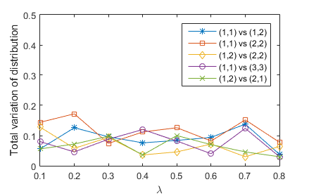
Since the allocation distributions for each element of the grid are visually similar looking, we compute the total variational distances between the distribution of different grid locations. These distances are used as a metric for us to determine whether two distributions are similar or not. For the 3x3 grid, grid locations $(1,1)$ , $(1,3)$ , $(3,1)$ and $(3,3)$ are statistically similar, as they are both on the corners of the area and share the same number of borders with the neighboring locations. By the same logic, grid locations $(1,2)$ , $(2,1)$ , $(2,3)$ and $(3,2)$ are also statistically similar. For statistically similar grids, we expect that the distributions of the allocations in these grid locations would be close to each other; note that this argument is only for the marginal distributions. In Figure 4 we find that the distance between allocation distributions on statistically dissimilar grid locations does not differ a lot from that of statistically similar ones. We believe this because the demand exceeds the supply so that all locations get fully subscribed.

However, as we notice from Figure 5 when the total demand exceeds the total supply, the prices at different grid locations show significant variations. The average prices of interior grid locations are generally higher than that of the grid locations on the boundary of the arena. We also observe that the larger the interference parameter $\lambda$ , the larger the difference in the average prices. This matches our intuition that the interior grids are generally more valuable since there are fewer boundaries with other locations, especially when the interference cost is large.

For the case $m_{g}=n_{g}=4,s_{g}=10,N_{a}=30,k_{a}=4,\mu=20$ , we also investigated the distribution of number of allocation on each grid. Here the total supply exceeds the total demand. Unlike the case when total demand exceeds the total supply, here we can see that the number of allocations differs significantly based on the grid locations (Figure 6). In general, the average number of allocations for interior grids are greater than that of the grids on the boundaries of the area. Here we do not display any statistics for the prices as they’re all uniformly low, as is to be expected.

3.2.4 Analysis of Shape of Bundles

We also investigate on the geometry of the bundles that the mechanism allocate to the users. Typically, bundles with more internal boundaries are more valuable than those with fewer internal boundaries. We expect that the mechanism would prefer to allocate bundles with more internal boundaries (such as ”O”-shaped 4-bundles), especially when the interference cost is high.

The empirical results agree with our intuition. As we observe from Figure 7, for the case where $m_{g}=n_{g}=3,s_{g}=10,N_{a}=30,k_{a}=4,\mu=20,\lambda=0.8$ , more 4-bundles are allocated than 3-bundles. Note that this is a setting where the demand exceeds the supply. Among all the 4-bundles that are allocated, bundles with more internal boundaries are significantly preferred by the mechanism, which means that the number of ”O”-shaped bundles of the resulting allocation is significantly higher than that of bundles of any other shape (”L”-shaped, ”T”-shaped, or ”Z”-shaped bundles).

We also investigate the case when $m_{g}=n_{g}=4,s_{g}=10,N_{a}=45,k_{a}=4,\mu=20,\lambda=0.8$ . In this case, nearly all assigned bundles are 4-bundles. Note that here the total supply exceeds the total demand. From Figure 8 we can see that most of the assigned 4-bundles has 4 internal boundaries, which means that they are ”O”-shaped. This again matches our intuition.

3.2.5 Analysis of Supporting Prices

We have theoretical guarantees that every agent obtains a bundle with his or her best possible payoff within some error $\epsilon_{u}$ . The error $\epsilon_{u}$ can be controlled by parameter $\delta_{w}$ . To verify this empirically we calculate the difference between the actual payoff an agent obtains and the best possible payoff. Theoretically, this difference should be larger than $-\epsilon_{u}$ , which is a very small number. Setting $\delta_{w}=10^{-5}$ , in the case of $m_{g}=n_{g}=3,s_{g}=10,N_{a}=45,k_{a}=4,\mu=20,\lambda=0.8$ , we observe in Figure 9 that in most cases the difference is 0; results of all iterations and all agents are pooled together in the figure. We also find that the minimum payoff difference we obtain in simulation is $-0.0011$ , which indicates a loss. However as we found the average actual payoff that agents obtain to be $4.123$ , we conclude that the loss is negligible. Actually, this loss can be arbitrarily small as we set $\delta_{w}$ to be small.

4 Implementation

We implemented the POPT mechanism as the Spectrum Allocation Tool in Python. It takes advantage of package CVXPY [11] and uses ECOS solver [14] to solve linear programming and quadratic programming problems, where ECOS is one of the most efficient solvers among all free solvers. The tool can be easily adapted to commercial solvers like GUROBI or MOSEK when these solvers are available to the user. The tool accepts two kinds of input: JSON and plain text. GUI input is currently not accepted as the input is usually some large data, which makes GUI input inconvenient. After calculation, the tool will visualize the resulting allocation scheme. The tool is open-source and is available at https://bitbucket.org/dwtang/batool .

5 Conclusion and Future Improvements

In this paper we proposed the POPT mechanism based on the OPT mechanism for matching problems where prices cannot be assessed [20], where we utilize prices to allocate goods to agents with complementarities in preferences. We have proved that the mechanism is approximately envy-free and asymptotically strategy-proof. We have also shown that the mechanism is approximately efficient in practice. Finally we implemented the mechanism as a GUI tool to enable practice of the mechanism in real world settings.

The POPT mechanism has a few nice properties. First, as the mechanism utilizes prices, envy-freeness emerges as a consequence and does not need to be imposed as a constraint in the underlying optimization problem. Furthermore, the prices for the mechanism are independent of what allocation the lottery scheme picks from the available allocation scheme set. Since the prices are the dual variables of the initial linear programming relaxation, we can calculate the prices at the same time of solving it, which makes the calculation of prices efficient.

In the future work, we plan on generalizing our mechanism to the case that each agent may desire more than one bundle. We also plan on determining theoretic guarantees on the efficiency of the mechanism using the optimal integer allocation with $k-1$ extra goods of each type.

References

[2] Moshe Babaioff, Brendan Lucier, Noam Nisan, and Renato Paes Leme. 2014. On the efficiency of the walrasian mechanism. In Proceedings of the fifteenth ACM conference on Economics and computation. ACM, 783–800.
[3] Yair Bartal, Rica Gonen, and Noam Nisan. 2003. Incentive compatible multi unit combinatorial auctions. In Proceedings of the 9th conference on Theoretical aspects of rationality and knowledge. ACM, 72–87.
[4] Randall Berry, Michael L Honig, and Rakesh Vohra. 2010. Spectrum markets: motivation, challenges, and implications. Communications Magazine, IEEE 48, 11 (2010), 146–155.
[5] Liad Blumrosen and Noam Nisan. 2007. Combinatorial auctions. Algorithmic game theory 267 (2007), 300.
[6] Jeremy Bulow, Jonathan Levin, and Paul Milgrom. 2009. Winning play in spectrum auctions. Technical Report. National Bureau of Economic Research.
[7] Peter Cramton. 1997. The FCC spectrum auctions: An early assessment. Journal of Economics & Management Strategy 6, 3 (1997), 431–495.
[8] Peter Cramton. 2002. Spectrum auctions. (2002).
[9] Peter Cramton, Andrzej Skrzypacz, and Robert Wilson. 2007. The 700 MHz spectrum auction: An opportunity to protect competition in a consolidating industry. (2007).
[10] Peter C Cramton, Yoav Shoham, Richard Steinberg, and others. 2006. Combinatorial auctions. Vol. 475. MIT press Cambridge.
[11] Steven Diamond, Eric Chu, and Stephen Boyd. 2014. CVXPY: A Python-Embedded Modeling Language for Convex Optimization, version 0.2. http://cvxpy.org/. (May 2014).
[12] Shahar Dobzinski and Noam Nisan. 2015. Multi-unit auctions: beyond Roberts. Journal of Economic Theory 156 (2015), 14–44.
[13] Shahar Dobzinski, Noam Nisan, and Michael Schapira. 2012. Truthful randomized mechanisms for combinatorial auctions. J. Comput. System Sci. 78, 1 (2012), 15–25.
[14] Alexander Domahidi, Eric Chu, and Stephen Boyd. 2013. ECOS: An SOCP solver for embedded systems. In Control Conference (ECC), 2013 European. IEEE, 3071–3076.
[15] David Easley and Jon Kleinberg. 2010. Networks, crowds, and markets: Reasoning about a highly connected world. Cambridge University Press.
[16] Venkatesan Guruswami, Jason D Hartline, Anna R Karlin, David Kempe, Claire Kenyon, and Frank McSherry. 2005. On profit-maximizing envy-free pricing. In Proceedings of the sixteenth annual ACM-SIAM symposium on Discrete algorithms. Society for Industrial and Applied Mathematics, 1164–1173.
[17] Vijay Krishna. 2009. Auction theory. Academic press.
[18] Paul Milgrom. 1998. Game theory and the spectrum auctions. European Economic Review 42, 3 (1998), 771–778.
[19] Ahuva Mu’Alem and Noam Nisan. 2008. Truthful approximation mechanisms for restricted combinatorial auctions. Games and Economic Behavior 64, 2 (2008), 612–631.
[20] Thành Nguyen, Ahmad Peivandi, and Rakesh Vohra. 2015. Assignment Problems with Complementarities. (2015).
[21] Thanh Nguyen and Rakesh Vohra. 2014. Near Feasible Stable Matchings with Complementarities. working paper (2014).
[22] Noam Nisan. 2000. Bidding and allocation in combinatorial auctions. In Proceedings of the 2nd ACM conference on Electronic commerce. ACM, 1–12.
[23] Noam Nisan and Amir Ronen. 2007. Computationally Feasible VCG Mechanisms. J. Artif. Intell. Res.(JAIR) 29 (2007), 19–47.
[24] Noam Nisan, Tim Roughgarden, Eva Tardos, and Vijay V Vazirani. 2007. Algorithmic game theory. Vol. 1. Cambridge University Press Cambridge.
[25] R Tyrrell Rockafellar and Roger J-B Wets. 2009. Variational analysis. Vol. 317. Springer Science & Business Media.
[26] Robert J Shapiro, Douglas Holtz-Eakin, and Coleman Bazelon. 2014. The economic implications of restricting spectrum purchases in the incentive auctions. Available at SSRN (2014).
[27] Rakesh Vohra and Lakshman Krishnamurthi. 2012. Principles of Pricing: an analytical approach. Cambridge University Press.
[28] Hang Zhou, Randall Berry, Michael L Honig, and Rakesh Vohra. 2013. Complexity of allocation problems in spectrum markets with interference complementarities. Selected Areas in Communications, IEEE Journal on 31, 3 (2013), 489–499.
[29] Günter M Ziegler. 1995. Lectures on polytopes. Vol. 152. Springer Science & Business Media.
[30] Edo Zurel and Noam Nisan. 2001. An efficient approximate allocation algorithm for combinatorial auctions. In Proceedings of the 3rd ACM conference on Electronic Commerce. ACM, 125–136.

APPENDIX

Appendix A Proof of Theorem 2.2

Let $x^{*}$ be one optimal solution for (LIP). Define set $S$ as

	$\displaystyle S=\Big\{$	$\displaystyle z\in\mathbb{R}^{\|N\|\times\|\mathcal{B}\|}~\Big\|~x^{*}_{i}(B)=0\Rightarrow z_{i}(B)=0,$
		$\displaystyle\sum_{i\in N}x^{*}_{i}(B)=1\Rightarrow\sum_{i\in N}z_{i}(B)=1,~z~\mathrm{satisfies~(Supply}+k-1)\Big\}$

Lemma A.1.

For any $z\in S$ that satisfies (Supply), we have $\overline{x}=\mathrm{IR}(z)\in S$ .

Proof A.2.

If $z\in S$ and $\overline{x}=\mathrm{IR}(z)$ , it follows from definition of $S$ as well as the procedure of Iterative Rounding (described in Section 2.2.1) that

	$\displaystyle x^{*}_{i}(B)$	$\displaystyle\Rightarrow z_{i}(B)=0\Rightarrow\overline{x}_{i}(B)=0$
	$\displaystyle\sum_{i\in N}x^{*}_{i}(B)=1$	$\displaystyle\Rightarrow\sum_{i\in N}z_{i}(B)=1\Rightarrow\sum_{i\in N}\overline{x}_{i}(B)=1$

If $z$ satisfies (Supply), from Theorem 2.1 it follows that $\overline{x}$ satisfies (Supply+ $k$ -1) (thus we have $\overline{s}_{j}\leq s_{j}+k-1$ ). Therefore, for any $z\in S$ that satisfies (Supply), we have $\overline{x}=\mathrm{IR}(z)\in S$ .

Then we will use induction to prove that $F\subseteq S$ after Lottery Construction procedure.

•

From Lemma A.1 we deduct that since $x^{*}\in S$ and $x^{*}$ satisfies (Supply), we have $x^{\prime},x^{\prime\prime}\in S$ . Hence, the initial $F^{(0)}\subseteq S$ .

•

Suppose that in the $p$ -th iteration of Lottery Construction we have $F^{(p)}\subseteq S$ . In this iteration, we have $y^{*}=\sum_{t=1}^{l}\lambda_{t}x^{t}$ , $\sum_{t=1}^{l}\lambda_{t}=1$ where $x^{t}\in S$ for $t=1,2,\cdots,l$ . As

	$\displaystyle x^{*}_{i}(B)=0$	$\displaystyle\Rightarrow x^{1}_{i}(B)=0,x^{2}_{i}(B)=0,\cdots,x^{l}_{i}(B)=0$
		$\displaystyle\Rightarrow y^{*}_{i}(B)=\sum_{j=1}^{l}\lambda_{j}x^{j}_{i}(B)=0$
	$\displaystyle\sum_{i\in N}x^{*}_{i}(B)=1$	$\displaystyle\Rightarrow\sum_{i\in N}x^{1}_{i}(B)=1,\sum_{i\in N}x^{2}_{i}(B)=1,\cdots,\sum_{i\in N}x^{l}_{i}(B)=1$
		$\displaystyle\Rightarrow\sum_{i\in N}y^{*}_{i}(B)=\sum_{t=1}^{l}\lambda_{t}\sum_{i\in N}x^{j}_{i}(B)=\sum_{t=1}^{l}\lambda_{t}=1$

and

	$\displaystyle\sum_{i\in N}\sum_{B\in\mathcal{B}}B_{j}y^{*}_{i}(B)$	$\displaystyle=\sum_{t=1}^{l}\lambda_{t}\left(\sum_{i\in N}\sum_{B\in\mathcal{B}}B_{j}x_{i}^{j}(B)\right)$
		$\displaystyle\leq\sum_{t=1}^{l}\lambda_{t}(s_{j}+k-1)=(s_{j}+k-1)\sum_{t=1}^{l}\lambda_{t}$
		$\displaystyle=s_{j}+k-1$

which means that $y^{*}$ satisfies (Supply+ $k$ -1). We then have $y^{*}\in S$ .

Then, as $z=x^{*}+\delta_{z}\frac{x^{*}-y^{*}}{\|x^{*}-y^{*}\|}$ , we have

$\displaystyle\sum_{i\in N}\sum_{B\in\mathcal{B}}B_{j}z_{i}(B)$	$\displaystyle=\sum_{i\in N}\sum_{B\in\mathcal{B}}B_{j}x^{}_{i}(B)+\delta_{z}\sum_{i\in N}\sum_{B\in\mathcal{B}}B_{j}\frac{x^{}_{i}(B)-y^{}_{i}(B)}{\\|x^{}-y^{*}\\|}$
	$\displaystyle\leq\tilde{s}_{j}+\dfrac{\delta_{\epsilon}\sum_{i\in N}\sum_{B\in\mathcal{B}}B_{j}(x^{}_{i}(B)-y^{}_{i}(B))}{\sqrt{\sum_{i\in N}\sum_{B\in\mathcal{B}}B_{j}^{2}}\cdot\\|x^{}-y^{}\\|}$
	$\displaystyle=s_{j}-\epsilon_{j}+\delta_{\epsilon}\dfrac{\overline{b}^{T}(x^{}-y^{})}{\\|\overline{b}\\|\cdot\\|x^{}-y^{}\\|}$	( $\overline{b}^{T}$ is the $j$ -th row vector of $B$ )
	$\displaystyle\leq s_{j}-\delta_{\epsilon}+\delta_{\epsilon}$	(Using Cauchy-Schwarz Inequality)
	$\displaystyle=s_{j}$

Thus $z$ satisfies (Supply). And as $y^{*}\in S$ we have

	$\displaystyle x^{*}_{i}(B)=0$	$\displaystyle\Rightarrow x_{i}^{}(B),y^{}_{i}(B)=0$
		$\displaystyle\Rightarrow z_{i}(B)=x^{}_{i}(B)+\delta_{z}\frac{x^{}_{i}(B)-y^{}_{i}(B)}{\\|x^{}-y^{*}\\|}=0$
	$\displaystyle\sum_{i\in N}x^{*}_{i}(B)=1$	$\displaystyle\Rightarrow\sum_{i\in N}x^{}_{i}(B)=1,\sum_{i\in N}y^{}_{i}(B)=1$
		$\displaystyle\Rightarrow\sum_{i\in N}z_{i}(B)=\sum_{i\in N}x^{}_{i}(B)+\delta_{z}\frac{\sum_{i\in N}x^{}_{i}(B)-\sum_{i\in N}y^{}_{i}(B)}{\\|x^{}-y^{*}\\|}$
		$\displaystyle~~~~~~~~~~~=1+\delta_{z}\cdot\frac{1-1}{\\|x^{}-y^{}\\|}=1$

Thus we have $z\in S$ . Therefore by Lemma A.1 $\overline{z}=\mathrm{IR}(z;c)\in S$ . Therefore, the updated ( $p+1$ -th iteration’s) $F^{(p+1)}=F^{(p)}\cup\{\overline{z}\}$ still satisfies $F^{(p+1)}\subseteq S$ .

Therefore we conclude that $F\subseteq S$ in all iterations. Thus the final set $F\subseteq S$ . This means that, any allocation vector $\overline{x}\in F$ satisfies

	$\displaystyle x^{*}_{i}(B)=0$	$\displaystyle\Rightarrow\overline{x}_{i}(B)=0,$
	$\displaystyle\sum_{i\in N}x^{*}_{i}(B)=1$	$\displaystyle\Rightarrow\sum_{i\in N}\overline{x}_{i}(B)=1$

From the definition of $\overline{s}_{j}$ we can see that

\displaystyle\sum_{i\in N}\sum_{B\in\mathcal{B}}B_{j}z_{i}(B)=\tilde{s}_{j}\Rightarrow\sum_{i\in N}\sum_{B\in\mathcal{B}}B_{j}\overline{x}_{i}(B)=\overline{s}_{j}

Denote the coefficient matrix of $x$ in constraints of (LIP) and (MLIP) as $A$ and the upperbound vector as $b$ for (LIP) and $\overline{b}$ for (MLIP). Then (LIP) can be denoted as $\displaystyle\max_{x\geq 0}\{u^{T}x:Ax\leq b\}$ and (MLIP) can be denoted as $\displaystyle\max_{x\geq 0}\{u^{T}x:Ax\leq\overline{b}\}$ . Then the above can be rewritten as

\displaystyle(Ax^{*}-b)_{k}=0\Rightarrow(A\overline{x}-\overline{b})_{k}=0

Since linear programming problems are convex problems, Karush-Kuhn-Tucker conditions are necessary and sufficient for optimality. Since $x^{*}$ is optimal for (LIP) we have the KKT condition: exist $\pi^{*},v^{*}\geq 0$ such that

	$\displaystyle-u+A^{T}\pi^{}-v^{}$	$\displaystyle=0$
	$\displaystyle{\pi^{}}^{T}(Ax^{}-b)$	$\displaystyle=0$
	$\displaystyle Ax^{*}$	$\displaystyle\leq b$
	$\displaystyle{v^{}}^{T}x^{}$	$\displaystyle=0$

By complementary slackness we have

	$\displaystyle v^{*}_{i}(B)$	$\displaystyle>0\Rightarrow z_{i}(B)=0\Rightarrow\overline{x}_{i}(B)=0$
	$\displaystyle\pi^{*}_{k}$	$\displaystyle>0\Rightarrow(Ax^{*}-b)_{k}=0\Rightarrow(A\overline{x}-\overline{b})_{k}=0$

Therefore we have

	$\displaystyle{v^{*}}^{T}\overline{x}$	$\displaystyle=0$
	$\displaystyle{\pi^{*}}^{T}(A\overline{x}-\overline{b})$	$\displaystyle=0$

And given the definition of $\overline{s}_{j}$ we can find that $\overline{x}$ is feasible for (MLIP), that is

\displaystyle A\overline{x}\leq\overline{b}

Thus we have KKT conditions also holds for $\overline{x}$ in (MLIP) (and the same Lagrange multipliers apply). Therefore $\overline{x}$ is an optimal solution to (MLIP).

As a result of the proof, we show that any dual variable of (LIP) is also a dual solution to (MLIP).∎

Appendix B Proof of Theorem 2.4

The dual problem of (MLIP) in Theorem 2.3 is given by

\displaystyle\begin{array}[]{ccll}&\displaystyle\min_{\alpha,p\geq 0}&\displaystyle\sum_{i\in N}\alpha_{i}+\displaystyle\sum_{j\in G}\overline{s}_{j}p_{j}\\ &\mathrm{s.t.}&\alpha_{i}\geq w_{i}(B)u_{i}(B)-\displaystyle\sum_{j\in G}B_{j}p_{j}&\forall i\in N,B\in\mathcal{B}\end{array}

(DMLIP)

where $\alpha_{i},\forall i\in N$ are the Lagrange multipliers associated with demand constraints of (MLIP), and $p_{j},\forall j\in G$ are the Lagrange multipliers associated with supply constraints of (MLIP).

As $\overline{x}$ is the optimal solution to the primal problem according to Theorem 2.3, we know that the dual problem must also have at least one optimal solution.

Suppose that $(\overline{\alpha},\overline{p})$ is an optimal solution for the dual problem, first we must have

\displaystyle\overline{\alpha}_{i}=\max_{B\in\mathcal{B}}\left\{w_{i}(B)u_{i}(B)-\sum_{j\in G}B_{j}\overline{p}_{j},0\right\}.

(If $\overline{\alpha}_{i}$ is less than the right hand side, then it is not feasible for the dual problem. If $\overline{\alpha}_{i}$ is larger than the right hand side, then the objective function value is larger)

By complementary slackness condition we have

	$\displaystyle\overline{x}_{i}(\hat{B})>0~~~$	$\displaystyle\Rightarrow~~~\overline{\alpha}_{i}=w_{i}(\hat{B})u_{i}(\hat{B})-\sum_{j\in G}\hat{B}_{j}\overline{p}_{j}$
	$\displaystyle\displaystyle\sum_{i\in N}\overline{x}_{i}(\hat{B})<1~~~$	$\displaystyle\Rightarrow~~~\overline{\alpha}_{i}=0$

Then we have

		$\displaystyle\mathrm{Agent~}i\mathrm{~gets~bundle~}\hat{B}$
	$\displaystyle\Rightarrow~~~$	$\displaystyle\overline{\alpha}_{i}=w_{i}(\hat{B})u_{i}(\hat{B})-\sum_{j\in G}\hat{B}_{j}\overline{p}_{j}=\max_{B\in\mathcal{B}}\left\{w_{i}(B)u_{i}(B)-\sum_{j\in G}B_{j}\overline{p}_{j}\right\}$
	$\displaystyle\Rightarrow~~~$	$\displaystyle u_{i}(\hat{B})-\sum_{j\in G}\hat{B}_{j}\overline{p}_{j}\geq u_{i}(B)-\sum_{j\in G}B_{j}\overline{p}_{j}$
		$\displaystyle~~~~~~~~~~~~~~~~~~~~~~-[(w_{i}(\hat{B})-1)u_{i}(\hat{B})+(1-w_{i}(B))u_{i}(B)]~~~\forall B\in\mathcal{B}$

		$\displaystyle\mathrm{Agent~}i\mathrm{~gets~no~bundle~}$
	$\displaystyle\Rightarrow~~~$	$\displaystyle\overline{\alpha}_{i}=0=\max_{B\in\mathcal{B}}\left\{w_{i}(B)u_{i}(B)-\sum_{j\in G}B_{j}\overline{p}_{j},0\right\}$
	$\displaystyle\Rightarrow~~~$	$\displaystyle w_{i}(B)u_{i}(B)-\sum_{j\in G}B_{j}\overline{p}_{j}\leq 0~~~\forall B\in\mathcal{B}$
	$\displaystyle\Rightarrow~~~$	$\displaystyle u_{i}(B)-\sum_{j\in G}B_{j}\overline{p}_{j}\leq(1-w_{i}(B))u_{i}(B)~~~\forall B\in\mathcal{B}$

Define $M_{i}=\max_{B\in\mathcal{B}}\{u_{i}(B)\}$ . Since $w_{i}$ is uniformly distributed in $[1-\delta_{w},1+\delta_{w}]$ we have the following

		$\displaystyle\mathrm{Agent~}i\mathrm{~gets~bundle~}\hat{B}$
	$\displaystyle\Rightarrow~~~$	$\displaystyle u_{i}(\hat{B})-\sum_{j\in G}\hat{B}_{j}\overline{p}_{j}\geq u_{i}(B)-\sum_{j\in G}B_{j}\overline{p}_{j}-2\delta_{w}M_{i}~~~\forall B\in\mathcal{B}$
		$\displaystyle\mathrm{Agent~}i\mathrm{~gets~no~bundle~}$
	$\displaystyle\Rightarrow~~~$	$\displaystyle u_{i}(B)-\sum_{j\in G}B_{j}\overline{p}_{j}\leq\delta_{w}M_{i}~~~\forall B\in\mathcal{B}$

By choosing $\delta_{w}$ to be small enough, we can make sure that $2\delta_{w}M_{i}\leq\epsilon_{u}$ for all $i\in N$ . Then we know that given the bundled price rule

\displaystyle\mathrm{Price}(B)=\sum_{j\in G}B_{j}\overline{p}_{j}

the agents would choose bundles that yields the best (within acceptable error) payoff, resulting in the designed allocation $\overline{x}$ . Thus, prices that support $\overline{x}$ exists.∎

Appendix C Proof of Theorem 2.7

Let $\alpha^{*}_{i}(i\in N)$ denote some Lagrange multipliers associated with demand constraints in (LIP) (such that $(\alpha^{*},p^{*})$ is an optimal solution for the dual of (LIP)), from complimentary slackness we know that

	$\displaystyle\alpha^{*}_{i}$	$\displaystyle=\max_{B\in\mathcal{B}}\left\{w_{i}(B)u_{i}(B)-\sum_{j\in G}B_{j}p_{j}^{*},0\right\}$
	$\displaystyle x^{*}_{i}(B)>0$	$\displaystyle\Rightarrow\alpha_{i}=w_{i}(B)u_{i}(B)-\sum_{j\in G}B_{j}p_{j}^{*}$
		$\displaystyle\Rightarrow w_{i}(B)u_{i}(B)-\sum_{j\in G}B_{j}p^{}_{j}=\max_{B\in\mathcal{B}}\left\{w_{i}(B)u_{i}(B)-\sum_{j\in G}B_{j}p_{j}^{}\right\}$

	$\displaystyle\sum_{i\in N}x^{*}_{i}(B)<1$	$\displaystyle\Rightarrow\alpha_{i}=0$
		$\displaystyle\Rightarrow w_{i}(B)u_{i}(B)-\sum_{j\in G}B_{j}p_{j}^{*}\leq 0~\forall B\in\mathcal{B}$

Define $M_{i}=\max_{B\in\mathcal{B}}\{u_{i}(B)\}$ . Consider two cases

•

$\displaystyle\sum_{i\in N}x_{i}^{*}(B)=1$

In this case we have

	$\displaystyle\sum_{B\in\mathcal{B}}[w_{i}(B)u_{i}(B)-P(B)]x_{i}^{*}(B)$	$\displaystyle=\sum_{B\in\mathcal{B}}\max_{B\in\mathcal{B}}\left\{w_{i}(B)u_{i}(B)-\sum_{j\in G}B_{j}p_{j}^{}\right\}x_{i}^{}(B)$
		$\displaystyle=\max_{B\in\mathcal{B}}\left\{w_{i}(B)u_{i}(B)-P(B)\right\}\cdot\sum_{B\in\mathcal{B}}x_{i}^{*}(B)$
		$\displaystyle=\max_{B\in\mathcal{B}}\left\{w_{i}(B)u_{i}(B)-P(B)\right\}\cdot 1$
		$\displaystyle\geq\max_{B\in\mathcal{B}}\left\{w_{i}(B)u_{i}(B)-P(B)\right\}\cdot\sum_{B\in\mathcal{B}}x_{k}^{*}(B)$
		$\displaystyle=\sum_{B\in\mathcal{B}}\max_{B\in\mathcal{B}}\left\{w_{i}(B)u_{i}(B)-P(B)\right\}x_{k}^{*}(B)$
		$\displaystyle\geq\sum_{B\in\mathcal{B}}[w_{i}(B)u_{i}(B)-P(B)]x_{k}^{*}(B)$

for all $i,k\in N$ .

As $w_{i}\geq 1-\delta_{w}$ , we then have

	$\displaystyle\sum_{B\in\mathcal{B}}[u_{i}(B)-P(B)]x_{i}^{*}(B)$	$\displaystyle\geq\sum_{B\in\mathcal{B}}[u_{i}(B)-P(B)]x_{k}^{*}(B)$
		$\displaystyle-\sum_{B\in\mathcal{B}}(1-w_{i}(B))u_{i}(B)[x^{}_{i}(B)-x^{}_{k}(B)]$
		$\displaystyle\geq\sum_{B\in\mathcal{B}}[u_{i}(B)-P(B)]x_{k}^{}(B)-\sum_{B\in\mathcal{B}}\delta_{w}M_{i}[x^{}_{i}(B)-x^{*}_{k}(B)]$
		$\displaystyle\geq\sum_{B\in\mathcal{B}}[u_{i}(B)-P(B)]x_{k}^{*}(B)-\delta_{w}M_{i}$

for all $i,k\in N$ , and by choosing $\delta_{w}$ small enough we can ensure that $\delta_{w}M_{i}\leq\epsilon_{u}$ for all $i\in N$ .

•

$\displaystyle\sum_{i\in N}x_{i}^{*}(B)<1$

In this case we have $x_{i}^{*}(B)>0\Rightarrow w_{i}u_{i}(B)-P(B)=0$

and $\sum_{i\in N}x_{i}^{*}(B)<1\Rightarrow w_{i}(B)u_{i}(B)-P(B)\leq 0~\forall B\in\mathcal{B}$ . Thus

\displaystyle\sum_{B\in\mathcal{B}}[w_{i}(B)u_{i}(B)-P(B)]x_{i}^{*}(B)

\displaystyle=0\geq\sum_{B\in\mathcal{B}}[w_{i}(B)u_{i}(B)-P(B)]x_{k}^{*}(B)

for all $i,k\in N$ .

As $w_{i}\geq 1-\delta_{w}$ we have

	$\displaystyle\sum_{B\in\mathcal{B}}[u_{i}(B)-P(B)]x_{i}^{*}(B)$	$\displaystyle\geq\sum_{B\in\mathcal{B}}[u_{i}(B)-P(B)]x_{k}^{*}(B)$
		$\displaystyle-\sum_{B\in\mathcal{B}}(1-w_{i}(B))u_{i}(B)[x^{}_{i}(B)-x^{}_{k}(B)]$
		$\displaystyle\geq\sum_{B\in\mathcal{B}}[u_{i}(B)-P(B)]x_{k}^{*}(B)-\delta_{w}M_{i}$

for all $i,k\in N$ , and by choosing $\delta_{w}$ small enough we can ensure that $\delta_{w}M_{i}\leq\epsilon_{u}$ for all $i\in N$ .

In all, we have the approximate envy-freeness condition holds.∎

Appendix D Proof of Polynomial Time

To prove that the algorithm is polynomial time, we first calculate the number of variables in (LIP).

Fix $k$ , the number of possible bundles in set $\mathcal{B}$ is given by

\displaystyle|\mathcal{B}|=\sum_{m=1}^{k}\begin{pmatrix}|G|+m-1\\ m\end{pmatrix}\sim O(|G|^{k})

Therefore the number of variables in (LIP) is given by

\displaystyle\mathrm{Nvar}=|N|\cdot|\mathcal{B}|\sim O(|N|\cdot|G|^{k})

The number of constraints in (LIP) is $|N|+|G|$ . Since linear programming problem can be solved (average case) in polynomial time with regard to number of variables and number of constraints, the first step of the algorithm can be finished in polynomial time.

For the iterative rounding process, in each iteration, either at least one variable is eliminated or at least one constraint is eliminated. So the number of rounds can not be larger than sum of the number of constraints and the number of variables.

In each round, a linear programming is performed, and it can be solved in polynomial time since its number of constraints and variables is polynomial. Therefore we conclude that the iterative rounding process is also polynomial time.

As the authors of [20] proved that the Lottery Construction procedure can finish in polynomial time, we conclude that the whole algorithm can be solved in polynomial time with regard to $|N|$ and $|G|$ .∎

Appendix E Proof of Theorem 3.2

Given the types of the agents, (LIP) is transformed to

\displaystyle\begin{array}[]{ccll}\mathrm{(LIP_{\Theta})}&\displaystyle\max_{x\geq 0}&\displaystyle\sum_{\theta\in\Theta}\sum_{B\in\mathcal{B}}w_{\theta}(B)u_{\theta}(B)y_{\theta}(B)&\\ &\mathrm{s.t.}&\displaystyle\sum_{B\in\mathcal{B}}\dfrac{1}{n_{\theta}}y_{\theta}(B)\leq 1&\theta\in\Theta\\ &&\displaystyle\sum_{\theta\in\Theta}\sum_{B\in\mathcal{B}}B_{j}y_{\theta}(B)\leq\tilde{s}_{j}&j\in G\end{array}

After figuring out an optimal solution $x^{*}$ for (LIP_Θ), individual shares are given by $x^{*}_{i}(B)=y^{*}_{\beta_{i}}(B)/n_{\beta_{i}}$ . In this sense (LIP_Θ) is equivalent to (LIP) since the symmetrical variables (shares of bundles of agents with same types) in (LIP) can have symmetrical optimal solutions. Therefore we will consider only the solutions of (LIP_Θ) in the following part.

The dual of (LIP_Θ) is given by

\displaystyle\begin{array}[]{ccll}\mathrm{(DLIP_{\Theta})}&\displaystyle\min_{\alpha,p\geq 0}&\displaystyle\sum_{\theta\in\Theta}\alpha_{\theta}+\displaystyle\sum_{j\in G}\tilde{s}_{j}p_{j}\\ &\mathrm{s.t.}&\dfrac{1}{n_{\theta}}\alpha_{\theta}\geq w_{\theta}(B)u_{\theta}(B)-\displaystyle\sum_{j\in G}B_{j}p_{j}&\theta\in\Theta,B\in\mathcal{B}\\ &&\alpha_{\theta}\leq M&\theta\in\Theta\end{array}

where $M$ is the optimal function value for (LIP_∞), which we will define later.

Note that the last constraint in the above problem is an additional constraint to ensure that the feasible region for the problem is bounded. Adding or deleting this constraint would not affect the optimal solution for the problem, as $M$ is greater or equal to the optimal solution of all (LIP_Θ), and there is no duality gap for linear programming problems, we have $M\geq\sum_{\theta\in\Theta}\alpha_{\theta}+\sum_{j\in G}s_{j}^{\prime}p_{j}\geq\alpha_{\theta}$ holds for $\theta\in\Theta$ even if we delete the third constraint. Thus this additional constraint is actually always true.

Consider an agent with type $\xi$ who misreports his type as $\zeta$ while others truthfully report their types, then we have the number of agent reporting each type to be

	$\displaystyle n_{\xi}^{\prime}$	$\displaystyle=n_{\xi}-1,~~~n_{\zeta}^{\prime}=n_{\zeta}+1,$
	$\displaystyle n_{\theta}^{\prime}$	$\displaystyle=n_{\theta}~~~\theta\in\Theta\backslash\{\xi,\zeta\}$

Then (LIP ${}_{\Theta}^{\prime}$ ) in this case is transformed to

\displaystyle\begin{array}[]{ccll}\mathrm{(LIP_{\Theta}^{\prime})}&\displaystyle\max_{x\geq 0}&\displaystyle\sum_{\theta\in\Theta}\sum_{B\in\mathcal{B}}w_{\theta}(B)u_{\theta}(B)y_{\theta}(B)&\\ &\mathrm{s.t.}&\displaystyle\sum_{B\in\mathcal{B}}\dfrac{1}{n_{\theta}^{\prime}}y_{\theta}(B)\leq 1&\theta\in\Theta\\ &&\displaystyle\sum_{\theta\in\Theta}\sum_{B\in\mathcal{B}}B_{j}y_{\theta}(B)\leq\tilde{s}_{j}&j\in G\end{array}

And the dual of (LIP ${}_{\Theta}^{\prime}$ ) is given by

\displaystyle\begin{array}[]{ccll}\mathrm{(DLIP_{\Theta}^{\prime})}&\displaystyle\min_{\alpha,p\geq 0}&\displaystyle\sum_{\theta\in\Theta}\alpha_{\theta}+\displaystyle\sum_{j\in G}\tilde{s}_{j}p_{j}\\ &\mathrm{s.t.}&\dfrac{1}{n_{\theta}^{\prime}}\alpha_{\theta}\geq w_{\theta}(B)u_{\theta}(B)-\displaystyle\sum_{j\in G}B_{j}p_{j}&\theta\in\Theta,B\in\mathcal{B}\\ &&\alpha_{\theta}\leq M&\theta\in\Theta\end{array}

When $n_{\theta}\rightarrow\infty$ for all $\theta\in\Theta$ , we have $n_{\theta}^{\prime}\rightarrow\infty$ for all $\theta\in\Theta$ and both (LIP_Θ) and (LIP ${}_{\Theta}^{\prime}$ ) converges to the following problem

\displaystyle\begin{array}[]{ccll}\mathrm{(LIP_{\infty})}&\displaystyle\max_{x\geq 0}&\displaystyle\sum_{\theta\in\Theta}\sum_{B\in\mathcal{B}}w_{\theta}(B)u_{\theta}(B)y_{\theta}(B)&\\ &\mathrm{s.t.}&\displaystyle\sum_{\theta\in\Theta}\sum_{B\in\mathcal{B}}B_{j}y_{\theta}(B)\leq\tilde{s}_{j}&j\in G\end{array}

And both (DLIP_Θ) and (DLIP ${}_{\Theta}^{\prime}$ ) converge to

\displaystyle\begin{array}[]{ccll}\mathrm{(DLIP_{\infty})}&\displaystyle\min_{\alpha,p\geq 0}&\displaystyle\sum_{\theta\in\Theta}\alpha_{\theta}+\displaystyle\sum_{j\in G}\tilde{s}_{j}p_{j}\\ &\mathrm{s.t.}&0\cdot\alpha_{\theta}\geq w_{\theta}(B)u_{\theta}(B)-\displaystyle\sum_{j\in G}B_{j}p_{j}&\theta\in\Theta,B\in\mathcal{B}\\ &&\alpha_{\theta}\leq M&\theta\in\Theta\end{array}

which is equivalent to the dual of (LIP_∞), i.e.

\displaystyle\begin{array}[]{ccll}\mathrm{(DLIP_{\infty})}&\displaystyle\min_{\alpha,p\geq 0}&\displaystyle\sum_{j\in G}\tilde{s}_{j}p_{j}\\ &\mathrm{s.t.}&0\geq w_{\theta}(B)u_{\theta}(B)-\displaystyle\sum_{j\in G}B_{j}p_{j}&\theta\in\Theta,B\in\mathcal{B}\end{array}

We have the following lemmas.

Lemma E.1.

With probability 1, (LIP_∞) and (DLIP_∞) both have a unique solution.

Proof E.2.

See Appendix F.

Lemma E.3.

For a sequence of optimization problems $P^{(n)}$ that have common continuous objective function, and the feasible regions $R^{(n)}$ are compact, converges, and satisfies the condition that $\bigcup_{n=1}^{\infty}R^{(n)}$ is bounded. Let $P*$ be an optimization problem with the same objective function as all $P^{(n)}$ and feasible region $R^{*}:=\displaystyle\lim_{n\rightarrow\infty}R^{(n)}$ . If $P^{*}$ has a unique optimal solution $y^{*}$ , then any sequence $y^{(n)}$ of solutions of $P^{(n)}$ must converge to $y^{*}$ .

Proof E.4.

See Appendix G.

Let $\mathbf{n}^{t}=(n_{\theta_{1}}^{t},n_{\theta_{2}}^{t},\cdots,n_{\theta_{m}}^{t})$ be any sequence of vectors such that $\mathbf{n}^{t}\rightarrow\infty$ as $t\rightarrow\infty$ . Denote the corresponding sequence of problems as (LIP_Θ)^t, (LIP ${}_{\Theta}^{\prime}$ )^t, (DLIP_Θ)^t, and (DLIP ${}_{\Theta}^{\prime}$ )^t respectively. And solution sequences for the problem sequences are $y_{\Theta}^{t}$ , $y_{\Theta}^{\prime t}$ , $p_{\Theta}^{t}$ , $p_{\Theta}^{\prime t}$ respectively.

We know that (LIP_∞) has a unique solution with probability 1. Since the union of feasible regions of (LIP_Θ)^t and (LIP ${}_{\Theta}^{\prime}$ )^t is a subset of feasible region of (LIP_∞), which is bounded, and the objective function are the same, we can apply Lemma C.2 and conclude that with probability 1, $y_{\Theta}^{t}$ and $y_{\Theta}^{\prime t}$ both converge to $y_{\Theta}^{*}$ , a solution of (LIP_∞).

Similarly, we know that (DLIP_∞) has a unique solution with probability 1. Since the union of feasible regions of (DLIP_Θ)^t and (DLIP ${}_{\Theta}^{\prime}$ )^t is a subset of feasible region of (DLIP ${}_{\Theta}~|~n_{\theta}=1\forall\theta\in\Theta$ ), which is bounded (with the additional constraint), and the objective functions are the same, we can apply Lemma C.2 and conclude that with probability 1, $p_{\Theta}^{t}$ and $p_{\Theta}^{\prime t}$ both converge to $p_{\Theta}^{*}$ , a solution of (DLIP_∞).

Then, apply Theorem 2.10 to (LIP ${}_{\Theta}^{\prime}$ )^t we have

\displaystyle\dfrac{1}{n_{\xi}^{\prime t}}\sum_{B\in\mathcal{B}}\left[u_{\xi}(B)-\sum_{j\in G}B_{j}p^{*}_{j}\right]y^{**(t)}_{\xi}(B)\geq\dfrac{1}{n_{\zeta}^{\prime t}}\sum_{B\in\mathcal{B}}\left[u_{\xi}(B)-\sum_{j\in G}B_{j}p^{*}_{j}\right]y^{**(t)}_{\zeta}(B)-\epsilon_{u}

(I)

where $y^{**(t)}$ is an optimal solution of (LIP ${}_{\Theta}^{\prime}$ )^t. Denote $y^{*(t)}$ as a solution for the corresponding original problem (LIP_Θ)^t. We have $y^{*(t)}$ and $y^{**(t)}$ converge to the same limit as $n_{\theta}\rightarrow\infty$ (with probability 1). Thus we have $\|y^{*(t)}-y^{**(t)}\|\rightarrow 0$ as $n_{\theta}\rightarrow\infty$ with probability 1. Denote the corresponding price vector as $p^{*(t)}$ and $p^{**(t)}$ . As $p^{*(t)}$ and $p^{**(t)}$ converge to the same limit, we also have $\|p^{*(t)}-p^{**(t)}\|\rightarrow 0$ as $n_{\theta}\rightarrow\infty$ with probability 1. Therefore we have for any $\varepsilon_{0}>0$ there exist $N_{0}$ such that when $n_{\theta}^{t}>N_{0}$ for all $\theta\in\Theta$ we have

	$\displaystyle\dfrac{1}{n_{\xi}^{t}}\sum_{B\in\mathcal{B}}\left[u_{\xi}(B)-\sum_{j\in G}B_{j}p^{(t)}_{j}\right]y^{(t)}_{\xi}(B)=\dfrac{1}{n_{\xi}^{\prime t}+1}\sum_{B\in\mathcal{B}}\left[u_{\xi}(B)-\sum_{j\in G}B_{j}p^{(t)}_{j}\right]y^{(t)}_{\xi}(B)$
$\displaystyle=~$	$\displaystyle\dfrac{1}{n_{\xi}^{\prime t}}\sum_{B\in\mathcal{B}}\left[u_{\xi}(B)-\sum_{j\in G}B_{j}p^{(t)}_{j}\right]y^{(t)}_{\xi}(B)-\dfrac{1}{n_{\xi}^{\prime t}(n_{\xi}^{\prime t}+1)}\sum_{B\in\mathcal{B}}\left[u_{\xi}(B)-\sum_{j\in G}B_{j}p^{(t)}_{j}\right]y^{(t)}_{\xi}(B)$
$\displaystyle\geq~$	$\displaystyle\dfrac{1}{n_{\xi}^{\prime t}}\left(\sum_{B\in\mathcal{B}}\left[u_{\xi}(B)-\sum_{j\in G}B_{j}p^{(t)}_{j}\right]y^{(t)}_{\xi}(B)-\dfrac{1}{2}\varepsilon_{0}\right)-o((n_{\xi}^{t})^{-1})$
$\displaystyle\geq~$	$\displaystyle\dfrac{1}{n_{\xi}^{\prime t}}\sum_{B\in\mathcal{B}}\left[u_{\xi}(B)-\sum_{j\in G}B_{j}p^{(t)}_{j}\right]y^{(t)}_{\xi}(B)-\varepsilon_{0}$	(II)

with probability 1.

Combining (I)(II) we get for any $\varepsilon_{0}>0$ there exist $N_{0}$ such that when $n_{\theta}>N_{0}$ for all $\theta\in\Theta$ we have

\displaystyle\dfrac{1}{n_{\xi}}\sum_{B\in\mathcal{B}}\left[u_{\xi}(B)-\sum_{j\in G}B_{j}p^{*}_{j}\right]y^{*}_{\xi}(B)\geq\dfrac{1}{n_{\zeta}^{\prime}}\sum_{B\in\mathcal{B}}\left[u_{\xi}(B)-\sum_{j\in G}B_{j}p^{**}_{j}\right]y^{**}_{\zeta}(B)-\epsilon_{u}-\varepsilon_{0}

with probability 1.

Since the final allocation of POPT is implemented as a lottery, where each agent of type $\theta$ has allocation vector with expectation $\frac{1}{n_{\theta}}y^{*}_{\theta}$ for (LIP_Θ) (or $\frac{1}{n_{\theta}^{\prime}}y^{**}_{\theta}$ , for (LIP ${}_{\Theta}^{\prime}$ )). Denote the final overall allocation vector as $\overline{x}$ for (LIP) and $\tilde{x}$ for (LIP’). Then we have for any $\varepsilon_{0}>0$ there exist $N_{0}$ such that when $n_{\theta}>N_{0}$ for all $\theta\in\Theta$ such that

\displaystyle\mathbb{E}\left\{\sum_{B\in\mathcal{B}}\left[u_{\beta_{i}}(B)-\sum_{j\in G}B_{j}p^{*}_{j}\right]\overline{x}_{\beta_{i}}(B)\right\}\geq\mathbb{E}\left\{\sum_{B\in\mathcal{B}}\left[u_{\beta_{i}}(B)-\sum_{j\in G}B_{j}p^{**}_{j}\right]\tilde{x}_{\zeta}(B)\right\}-\epsilon_{u}-\varepsilon_{0}

Proving the result.∎

Appendix F Proof of Lemma D.1

In (LIP_∞) we have two set of parameters controlled by random variables: $w_{i}(B)\sim\mathcal{U}(1-\delta_{w},1+\delta_{w})$ , and $\tilde{s}_{j}\sim\mathcal{U}(s_{j}-2\delta_{\epsilon},s_{j}-\delta_{\epsilon})$ . All of the random variables are independent.

The constraints of (LIP_∞) defines a (bounded) polytope with finite number of extreme points. Denote $\{q^{1},q^{2},\cdots,q^{m}\}$ as the set of extreme points, we can see that $q^{1},q^{2},\cdots,q^{m}$ are random variables that depend only on $s_{j}^{\prime}$ for $j\in G$ .

Therefore, $q^{1},q^{2},\cdots,q^{m}$ are independent of $w_{i}(B)$ for $i\in N,B\in\mathcal{B}$ . Define $v^{1},v^{2},\cdots,v^{m}$ such that $v^{t}_{i}(B)=q^{t}_{i}(B)u_{i}(B)$ for $t=1,2,\cdots,m$ . As $q_{s}\neq q_{t}$ for $s\neq t$ and $u_{i}(B)>0$ , we have $v_{s}\neq v_{t}$ for $s\neq t$ . Then we can express the objective function value at $q^{t}$ as $w^{T}q^{t}$ .

Then we have for any $s\neq t$ , $s,t=1,2,\cdots,m$ ,

\displaystyle\Pr[w^{T}q^{s}=w^{T}q^{t}]=\Pr[w^{T}(q^{s}-q^{t})=0]

Since $(q^{s}-q^{t})$ is a non-zero vector which is independent of $w$ , $w^{T}(q^{s}-q^{t})$ is a continuous random variable. Then the probability that this random variable has a specific value is 0. Thus

\displaystyle\Pr[w^{T}q^{s}=w^{T}q^{t}]=0

It follows that

\displaystyle\Pr[w^{T}q^{s}\neq w^{T}q^{t}~\forall s\neq t]=1

A lemma in [29] states that a sufficient condition for the uniqueness of a solution for a linear programming problem is that $w^{T}q^{s}\neq w^{T}q^{t}$ for all $t\neq s$ , $s,t=1,2,\cdots,m$ . Therefore, with probability 1, we have (LIP_∞) to have a unique solution.∎

Similarly, in (DLIP_∞) we have a set of parameters controlled by random variables: $\tilde{s}_{j}\sim\mathcal{U}(s_{j}-2\delta_{\epsilon},s_{j}-\delta_{\epsilon})$ . All of the random variables are independent. The constraints defines a bounded polytope with finite number of extreme points. The coordinates of the extreme points is a constant (hence independent of $\tilde{s}_{j}$ ). Then, follow a similar proof for (DLIP_∞), we conclude that (DLIP_∞) has a unique solution with probability 1.

Therefore, with probability 1, (LIP_∞) and (DLIP_∞) both have a unique solution.∎

Appendix G Proof of Lemma D.2

Denote the objective function of $P^{(n)}$ and $P^{*}$ as $f$ , and a sequence of solution of $P^{(n)}$ as $y^{(n)}$ . Denote the unique solution of $P^{*}$ as $y^{*}$

For the sequence of optimization problems $P^{(n)}$ and $P^{*}$ , if $P^{*}$ has solutions, then by Berge’s Maximum Theorem the optimal objective function values of $P^{(n)}$ converges to the optimal objective function value of $P^{*}$ . That is $f(y^{(n)})\rightarrow f(y^{*})$ as $n\rightarrow\infty$ .

Suppose that $y^{(n)}$ does not converge to $y^{*}$ , which means that there exists some $\varepsilon>0$ such that there exists a subsequence $y^{(n_{k})}$ satisfies

\displaystyle\|y^{(n_{k})}-y^{*}\|>\varepsilon

However, $y^{(n_{k})}$ is bounded. By Bolzano-Weierstrass Theorem, there exist a subsequence $y^{(n_{k_{t}})}$ of $y^{(n_{k})}$ such that $y^{(n_{k_{t}})}$ converges to some point $\tilde{y}$ . By the definition of set convergence [25] the feasible regions $R^{(n_{k_{t}})}$ converges to the feasible region $R^{*}$ of $P^{*}$ .

\lim_{t\rightarrow\infty}R^{(n_{k_{t}})}=\limsup_{t\rightarrow\infty}R^{(n_{k_{t}})}=R^{*}

By definition of limits of sets [25], we have $\tilde{y}\in\limsup_{t\rightarrow\infty}R^{(n_{k_{t}})}$ thus $\tilde{y}\in R^{*}$ . Since the objective function is continuous, we have $f(y^{(n_{k_{t}})})$ converges to $f(\tilde{y})$ .

Since $y^{(n_{k_{t}})}$ is a subsequence of $y^{(n)}$ and $f(y^{(n)})$ converges to $f(y^{*})$ , we have $f(y^{(n_{k_{t}})})$ converges to $f(y^{*})$ . Therefore $f(\tilde{y})=f(y^{*})$ , which means that $\tilde{y}$ is also an optimal solution of $P^{*}$ .

However $y^{*}\neq\tilde{y}$ , as $\|\tilde{y}-y^{*}\|=\displaystyle\lim_{t\rightarrow\infty}\|y^{(n_{k_{t}})}-y^{*}\|\geq\varepsilon>0$ . Thus $\tilde{y}$ is an optimal solution different from $y^{*}$ . This contradicts with the condition that $y^{*}$ is the unique solution for $P^{*}$ .

Therefore $y^{(n)}$ must converge to $y^{*}$ .∎

	$\displaystyle x^{*}_{i}(B)=0$	$\displaystyle\Rightarrow x_{i}^{}(B),y^{}_{i}(B)=0$
		$\displaystyle\Rightarrow z_{i}(B)=x^{}_{i}(B)+\delta_{z}\frac{x^{}_{i}(B)-y^{}_{i}(B)}{\\|x^{}-y^{*}\\|}=0$
	$\displaystyle\sum_{i\in N}x^{*}_{i}(B)=1$	$\displaystyle\Rightarrow\sum_{i\in N}x^{}_{i}(B)=1,\sum_{i\in N}y^{}_{i}(B)=1$
		$\displaystyle\Rightarrow\sum_{i\in N}z_{i}(B)=\sum_{i\in N}x^{}_{i}(B)+\delta_{z}\frac{\sum_{i\in N}x^{}_{i}(B)-\sum_{i\in N}y^{}_{i}(B)}{\\|x^{}-y^{*}\\|}$
		$\displaystyle~~~~~~~~~~~=1+\delta_{z}\cdot\frac{1-1}{\\|x^{}-y^{}\\|}=1$