Gamma-Ray Bursts from Magnetic Reconnection: Variability and Robustness of Lightcurves
Abstract
The dissipation mechanism that powers gamma-ray bursts (GRBs) remains uncertain almost half a century after their discovery. The two main competing mechanisms are the extensively studied internal shocks and the less studied magnetic reconnection. Here we consider GRB emission from magnetic reconnection accounting for the relativistic bulk motions that it produces in the jet’s bulk rest frame. Far from the source the magnetic field is almost exactly normal to the radial direction, suggesting locally quasi-spherical thin reconnection layers between regions of oppositely directed magnetic field. We show that if the relativistic motions in the jet’s frame are confined to such a quasi-spherical uniform layer, then the resulting GRB lightcurves are independent of their direction distribution within this layer. This renders previous results for a delta-function velocity-direction distribution [6] applicable to a much more general class of reconnection models, which are suggested by numerical simulations. Such models that vary in their velocity-direction distribution differ mainly in the size of the bright region that contributes most of the observed flux at a given emission radius or observed time. The more sharply peaked this distribution, the smaller this bright region, and the stronger the lightcurve variability that may be induced by deviations from a uniform emission over the thin reconnection layer, which may be expected in a realistic GRB outflow. This is reflected both in the observed image at a given observed time and in the observer-frame emissivity map at a given emission radius, which are calculated here for three simple velocity-direction distributions.
Subject headings
Gamma-ray burst: general — magnetic reconnection — magnetohydrodynamics (MHD) — relativistic processes — methods: analyticalI. Introduction
Gamma-ray Bursts (GRBs) are the most luminous cosmic explosions, with huge isotropic-equivalent luminosities of [41, 28, for a review see, e.g.,]. They divide into two main sub-classes [26]: long-duration (s) soft-spectrum GRBs that are associated with broad-lined SNe Ic, implying a massive-star progenitor [49, e.g.,], and short-duration (s) hard-spectrum GRBs that are thought to arise from the merger of a binary neutron-star system or a neutron star and a stellar-mass black hole [11, 39, 31, 38]. In both classes the central engine is a newly formed rapidly accreting stellar-mass black hole or a rapidly rotating highly magnetized neutron star (millisecond magnetar), which launches a relativistic jet.
The bright GRB prompt -ray emission shows rapid variability and typically peaks at photon energies of hundreds of keV. This would imply a huge optical depth to pair production, which is incompatible with its non-thermal spectrum (the compactness problem), unless the emitting region moves toward us with an ultra-relativistic Lorentz factor of [4, 36, 17, 23]. Such a highly relativistic outflow also naturally explains the subsequent afterglow emission in X-ray, optical and radio over days, weeks and months after the GRB, as the ejecta are decelerated by the external medium and drive a long-lived shock into it, which gradually decelerates as it sweeps-up more mass. Compactness arguments also require a large enough prompt emission radius (cm) in particular for the GeV photons detected by Fermi in some GRBs [1, 2, 3, e.g.,]. The observed fast variability of the GRB prompt emission implies that it must be produced by internal dissipation within the ejecta [43].
The GRB outflow composition, as well as the dissipation and emission mechanisms that produce the prompt emission are still uncertain, and are important open questions in this field. They can also affect each other, as the outflow composition affects its dynamics and dissipation, which in turn affect the resulting emission. In particular, a key question is whether the energy is carried out from the central source to the emission region predominantly as kinetic energy – a baryonic jet [13, 40, 44], or as Poynting flux – a highly magnetized (or Poynting-flux dominated) jet [48, 47, 37, 7, 34, 20] with a large magnetization parameter (the magnetic-to-particle enthalpy density or energy flux ratio). A baryonic, kinetically dominated jet can naturally lead to reasonably efficient energy dissipation via internal shocks within the outflow [42]. This may also occur in an initially high- outflow that is highly variably, due to impulsive acceleration that converts its initial magnetic energy into kinetic energy [18, 16]. As long as the flow remains highly magnetized this suppresses internal shocks. On the other hand, in high- outflows there is an alternative dissipation mechanism that can be more efficient than internal shocks – magnetic reconnection [47, 46, 35, 12, 33, 24].
A high near the central source can help avoid excessive baryon loading that might prevent the jet from reaching sufficiently high Lorentz factors far from the source, at the emission region. Such initially high- jets are also favored on energetic grounds, since modeling of GRB central engines that rely on hydromagnetic jet launching via accretion disks suggest that their power is significantly larger than that of thermally driven outflows powered by neutrino-anti neutrino annihilation [25, e.g.,], and they may naturally lead to magnetic reconnection.
In a striped wind magnetic field configuration [10, e.g.], whether the flipping of the magnetic field direction near the source is periodic (as expected for a millisecond-magnetar central engine) or stochastic (as expected for an accreting black hole), reconnection at large distances from the source has a natural preferred direction. At such large distances the magnetic field is almost exactly normal to the (spherical) radial direction, as are the current sheets that separate regions of opposite magnetic polarity where reconnection occurs, thus forming nearly spherical thin reconnection layers. Moreover, for a large just before the dissipation region reconnection leads to local relativistic bulk motion of the outgoing particles away from the reconnection sites in the jet’s bulk frame, with a Lorentz factor that can reach a few to several. This leads to anisotropic emission in the jet’s bulk frame, which can significantly affect the observed emission.
Figure 1 (bottom panel) shows a simple manifestation of our basic model where the jet consists of shells with oppositely oriented toroidal magnetic field, separated by quasi-spherical current sheets where reconnection occurs (a modest poloidal field-component should not significantly change this basic picture). In GRBs the jet half-opening angle typically satisfies so only a small fraction of the jet (; the green circle in Figure 1) is visible, and the magnetic field may be approximated as uniform within it. This approximation was made for calculating the prompt-GRB polarization [14, 19], and should not greatly affect our results. For the afterglow polarization the global toroidal-field structure was considered [30, 21] since the whole jet becomes visible as it decelerates during the afterglow. Anisotropic synchrotron emission was considered as a possible cause of early X-ray afterglow variability or rapid decay [5]. We allow for any reconnection-induced velocity-direction distribution in the jet’s bulk frame within the quasi-spherical reconnection layer ( is defined in Figure 1, top panel). Such an anisotropic emission model was recently considered for the prompt-GRB emission by Beniamini & Granot 6 (hereafter BG16), where velocities are in the direction of the anti-parallel magnetic-field lines just prior to their reconnection, which is uniform within visible region.
Our anisotropic emission model differs from previous relativistic-turbulence models [35, 27, 29] that assume an isotropic velocity distribution of the motions in the jet’s bulk frame. For this model BG16 calculated the expected lightcurves and spectra of the prompt emission, and demonstrated that it can potentially reproduce many of the observed prompt GRB properties (e.g. its variability, pulse asymmetry, the very rapid decay phase at its end, and many of the observed correlations).
Recent simulations of relativistic magnetic reconnection suggest that as increases, both the reconnection rate and resulting particle bulk velocities () increase, and the power-law index of their energy spectrum becomes harder [8, 9, 45, 22, 24, 32]. In high- GRB outflows one may typically expect a few to several. The collimation of the accelerated electrons appears to increase with their energy. Their velocities are indeed predominantly confined to the reconnection layer, but are not necessarily along the anti-parallel directions of the magnetic field lines just before the reconnection (as was assumed by BG16). This motivates us to consider such velocity distributions that are more general.
In Section II the lightcurve is shown to be independent of the angular distribution of the velocities in the jet’s bulk frame as long as they are confined to a uniformly emitting spherical reconnection layer; does, however, affect the observed image and the contribution to the observed flux from a given emission radius, which are calculated in Sections III and IV, respectively. This may in turn affect the prompt GRB lightcurve if the emission across the spherical reconnection layer is non-uniform, which may be expected under realistic conditions. Finally, the main results are summarized and discussed in Section V.
II. Flux Density is Independent of Velocity Directions within a Uniform Spherical Reconnection Layer
Here we show that the observed flux density at any observed frequency and time is independent of the velocity-direction distribution of the emitting plasma within a uniform spherical thin reconnection layer. Let be such a general probability distribution (normalized as ) of local velocity directions in the jet’s bulk frame (that is primed in Figure 1, top panel) that are at angles relative to the local direction of the magnetic field ( in Figure 1, which is a preferred direction within the reconnection layer, and is assumed here to be uniform within the visible region). We follow the notations of BG16 (e.g., in the source’s frame is the polar angle measured from the line of sight, and is the azimuthal angle). The general expression for the flux density is then given by a weighted average over that for a single velocity direction taken from BG16,
| (1) | |||||
where is the effective distance to the source and is the luminosity distance, is the normalized radius, for a blob and for a steady state in the jet’s frame, , is the Doppler factor between the rest frame of the central source and the jet’s bulk frame, is the Doppler factor between the jet’s bulk frame and the local emitting plasma’s rest frame (it depends on through ), and where is the frequency in the source’s cosmological frame. Thus, the only dependence on the azimuthal angle is through , both directly and through , and this dependence is in turn only through . Therefore, one can reverse the order of integration over and , and change variables from to ,
| (2) |
where the inner integral over is independent of , so that the outer integral over gives 1 from the normalization of . This reduces the expression for the observed flux density to that for a delta function in velocity direction (e.g. in Eq. [4]) as in BG16, where one can take ,
| (3) |
The reason why the observed flux is independent of is as follows. The observed flux is the weighted mean of the contributions from plasma with different velocity directions . However, the observed flux from such a uni-directional distribution does not depend on its absolute direction , since the latter affects only the dependence of the observed radiation on the azimuthal angle , and thus the observed image, but not the photon arrival times or the observed flux density.
III. The Observed Image for Anisotropic Emission
This motivates us to calculate the observed image for different choices of and . For comparison we will also show the image for isotropic emission in the jet’s bulk frame (), from [15]. In particular, we will use
| (4) |
where (used in BG16) corresponds to velocity along the anti-parallel reconnecting magnetic field lines, is motivated by PIC simulations of relativistic reconnection, and is the extreme assumption of a uniform velocity distribution within the thin reconnection layer. For each of these we calculate the image for .
The flux density differential is , where is the angular distance to the source and is the area of the image, normal to the line of sight. If is the corresponding distance from the center of the image, then
| (5) |
where . We are interested in the specific intensity at a general location within the image, , where
| (6) |
and . As we evaluate at a fixed , one still needs to integrate over , or more conveniently switch variables to and obtain
| (7) |
| (8) | |||||
Now we shall use the expressions for the relevant terms,
| (9) |
| (10) |
Now, for simplicity, we shall specify to a power-law spectrum, , and emission with radius, between and , with a constant and , 11 1 This result reduces to Eq. (15) of [15] for isotropic emission in the jet’s bulk frame (), with the small modifications given in Eqs. (8) and (17) therein, which reflect the difference between a shock and a reconnection layer. To match the notations there one should take and where there is the power-law index of the external density profile in front of the afterglow shock.
| (11) |
Each corresponds to two values of , at the front () and the back () of the equal arrival time surface of photons to the observer. They are generally found by numerically solving Eq. (6), but for some -values can be found analytically [15], e.g. and . One must add up these two contributions to . There is contribution only from radii corresponding to where and . In the following, for simplicity, emission is assumed from all radii.
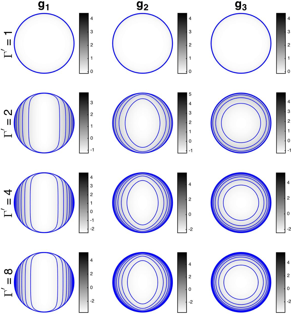
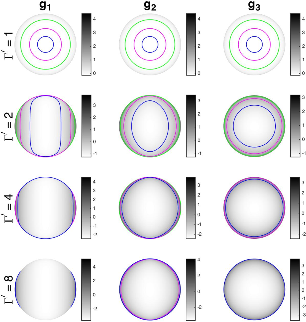
The resulting images are shown in Figs. 2 and 3. Figure 2 adds equally spaced contour lines, with . Figure 5 adds contour lines at values above which 50% (green), 80% (magenta), and 95% (blue) of the total flux originates. For most of the flux clearly comes from a small part of the image near its outer edge. For (a delta-function anti-parallel velocity distribution) most of the flux comes from two small regions near the outer edge of the image, which quickly decrease in size as increases. For most of the flux comes from an asymmetric ring at the outer edge of the image. For (an isotropic velocity distribution within the reconnection layer – normal to the radial direction) this ring becomes symmetric about the center of the image, following the behavior of the whole image in this case for which there is no preferred -direction.
IV. Contribution to Observed Flux from a Given Radius
It is also useful to examine the contribution to the observed flux from a given emission radius (as a function of and ) even though it arrives over a range of observed times . To this end we consider the contribution per unit area of the shell at a constant and , where
| (12) |
Altogether, for a power-law emission spectrum one obtains
| (13) |
The integrals over in Eqs. (11) and (13), for , generally give hypergeometric functions for . However, for integer values they become particularly simple. E.g., for , and , where is given by
| (14) |
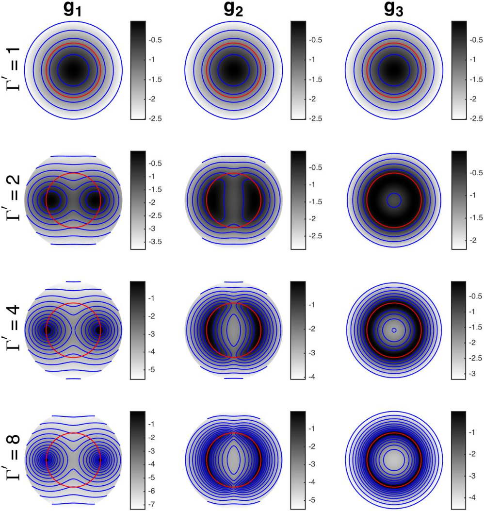
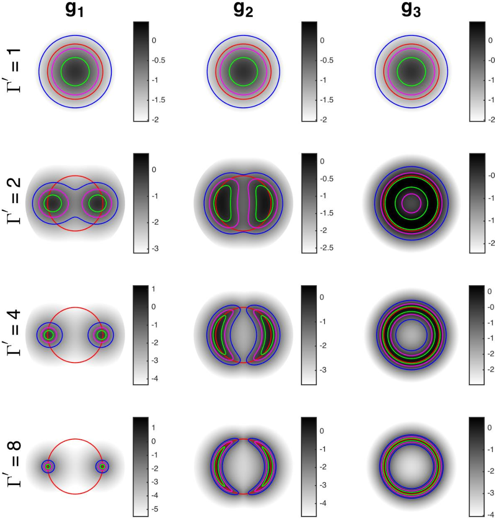
Figures 4 and 5 show logarithmic color maps of , the contribution to the observed flux density per unit area of the emitting shell from a given radius, according to Eq. (13). Figure 4 adds equally spaced contour lines, with . Figure 5 adds contour lines at the values above which 50% (green), 80% (magenta), and 95% (blue) of the total flux from the given emission radius originates.
V. Discussion
In Section II it was shown that the observed flux density (and thus the lightcurves and spectra) of GRB prompt emission from a uniform spherical thin reconnection layer are independent of the distribution of velocity directions within this layer in the jet’s bulk frame. This implies that the detailed results for the lightcurves, spectra, and temporal-spectral correlations of BG16, who assumed velocities along two anti-parallel directions, are valid for a much larger class of reconnection models, which is consistent with the results of recent simulations.
In Sections III and IV it was shown that as increases, the size of the “bright part” within the observed region of the reconnection layer that contributes most of the observed flux becomes significantly smaller. Moreover, its area and angular size depend on the spread of , as expressed in the angular distribution . For a few, for the tightest angular distribution we considered of two anti-parallel directions ( in Equation (4)) most of the observed flux comes from two small circular regions of angular size (see left panels of Figure 5), which occupy a fraction of the visible region. On the other extreme, for our most spread-out velocity distribution that is uniform within the reconnection layer ( in Equation (4)), most of the flux comes from a thin ring of angular radius and width (see right panels of Figure 5), occupying a fraction of the visible region. These results should not significantly change when relaxing our approximation of a uniform magnetic field within the visible region.
These results may be important if the emission over the spherical thin reconnection layer is not uniform but has some angular dependence, e.g. due to irregularities or non-uniformity in the reconnection rate. The value of affects (which determines the size of the region contributing most of the observed flux), the reconnection rate (which affects the local radiated power per unity area in the reconnection layer), as well as the electron energy distribution that affects the emission spectrum (and hence the observed spectrum and flux at a given observed energy range). Since may vary with the angular location within the outflow, or even with time at a fixed angular location, one might expect that this could potentially lead to significant angular inhomogeneities in the emission from a given radius, as well as temporal changes at a given angular location.
If the prompt emission occurs when the jet is coasting at a constant then the angular location of the “bright part” (which is at an angle of from the line of sight) is fixed in time and the lightcurve variability reflects mainly the radial profile of the emission within this small region. If, on the other hand, the jet is still accelerating or conversely starting to decelerate during the reconnection, then the “bright part” will scan through different angular locations and the lightcurve variability could also reflect the angular distribution of the spectral emissivity in the reconnection layer. In all cases, the larger this “bright part” (i.e. the smaller or , and the wider the velocity spread ) the more it might average out over different local fluctuations or angular inhomogeneities in the emission, thus reducing the lightcurve variability. Conversely, a larger lightcurve variability may be expected for a smaller “bright part” (i.e. a larger or , and a narrower velocity spread ), due to less averaging out, and a larger sensitivity to fluctuations in the emission over small times or angular scales. A more detailed and quantitative study of these effects on the observed prompt GRB emission is planned in a future work.
References
- [1] Abdo, A. A., et al., 2009, ApJ, 707, 580
- [2] Abdo, A. A., et al., 2010, ApJ, 712, 558
- [3] Ackermann, M., et al., 2013, ApJS, 209, 11
- [4] Baring, M. G., & Harding, A. K. 1997, ApJ, 491, 663
- [5] Beloborodov, A. M., Daigne, F., Mochkovitch, R., & Uhm, Z. L. 2011, MNRAS, 410, 2422
- [6] Beniamini, P., & Granot, J. 2016, MNRAS, 459, 3635
- [7] Blandford, R. D. 2002, in “Lighthouses of the Universe: The Most Luminous Celestial Objects and Their Use for Cosmology”, ed. by M. Gilfanov, R. Sunyeav, E. Churazov, p. 381
- [8] Cerutti, B., Werner, G. R., Uzdensky, D. A., & Begelman, M. C. 2012, ApJL, 754, L33
- [9] Cerutti, B., Werner, G. R., Uzdensky, D. A., & Begelman, M. C. 2014, ApJ, 782, 104
- [10] Coroniti F. V. 1990, ApJ, 349, 538
- [11] Eichler, D., Livio, M., Piran, T., & Schramm, D. N. 1989, Nature, 340, 126
- [12] Giannios, D., & Spruit, H. C. 2007, A&A, 469, 1
- [13] Goodman, J. 1986, ApJL, 308, L47
- [14] Granot, J. 2003, ApJL, 596, L17
- [15] Granot, J. 2008, MNRAS, 390, L46
- [16] Granot, J. 2012, MNRAS, 421, 2467
- [17] Granot, J., Cohen-Tanugi, J., & do Couto e Silva, E., 2008, ApJ, 677, 92
- [18] Granot, J., Komissarov, S. S., & Spitkovsky, A. 2011, MNRAS, 411, 1323
- [19] Granot, J., & Königl, A. 2003, ApJL, 594, L83
- [20] Granot, J., Piran, T., Bromberg, O, Racusin, J. L., & Daigne, F. 2015, in The Strongest Magnetic Fields in the Universe, Vol. 54, ed. A. Balogh et al. (Berlin: Springer), 471
- [21] Granot, J., & Taylor, G. B. 2005, ApJ, 625, 263
- [22] Guo, F., Liu, Y.-H., Daughton, W., & Li, H. 2015, ApJ, 806, 167
- [23] Hascoët, R., Daigne, F., Mochkovitch, R., & Vennin, V. 2012, MNRAS, 421, 525
- [24] Kagan, D., Sironi, L., Cerutti, B., & Giannios, D. 2015, in The Strongest Magnetic Fields in the Universe, Vol. 54, ed. A. Balogh et al. (Berlin: Springer), 545
- [25] Kawanaka N., Piran T., & Krolik J. H., 2013, ApJ, 766, 31
- [26] Kouveliotou, C., et al. 1993, ApJL, 413, L101
- [27] Kumar P., Narayan R., 2009, MNRAS, 395, 472
- [28] Kumar, P., & Zhang, B. 2015, Phys. Rep., 561, 1
- [29] Lazar, A., Nakar, E., & Piran, T. 2009, ApJL, 695, L10
- [30] Lazzati, D., et al. 2004, A&A, 422, 121
- [31] Lee, W. H., & Ramirez-Ruiz, E. 2007, New J. Phys., 9, 17
- [32] Liu, Y.-H., Guo, F., Daughton, W., Li, H., & Hesse, M. 2015, PRL, 114, 095002
- [33] Lyubarsky, Y. E. 2010, ApJL, 725, L234
- [34] Lyutikov, M. 2006, New J. Phys., 8, 119
- [35] Lyutikov, M., & Blandford, R. 2003, arXiv:astro-ph/0312347
- [36] Lithwick, Y., & Sari R., 2001, Astrophys. J. 555, 540.
- [37] Mészáros, P., & Rees, M. J. 1997, ApJL, 482, L29
- [38] Nakar, E. 2007, Phys. Rep., 442, 166
- [39] Narayan, R., Paczýnski, B., & Piran, T. 1992, ApJL, 395, L83
- [40] Paczýnski, B. 1986, ApJL, 308, L43
- [41] Piran T., 2004, Rev. Mod. Phys., 76, 1143
- [42] Rees, M. J., & Mészáros, P., 1994, ApJL, 430, L93
- [43] Sari, R., & Piran, T. 1997, ApJ, 485, 270
- [44] Shemi, A., & Piran, T. 1990, ApJL, 365, L55.
- [45] Sironi, L., & Spitkovsky, A. 2014, ApJL, 783, L21
- [46] Spruit, H. C., Daigne, F., & Drenkhahn, G. 2001, A&A, 369, 694
- [47] Thompson, C. 1994, MNRAS, 270, 480
- [48] Usov, V. V. 1992, Nature, 357, 472
- [49] Woosley S. E., Bloom J. S., 2006, ARA&A, 44, 507