Grid-like structure is optimal for path integration

Grid cells in medial entorhinal cortex (MEC) are believed to play a key role in computations underlying path integration [4, 8]. However, the relation between their grid-like firing field and path integration is not clear. Previous studies have shown that grid-like pattern can emerge from the interference of two or more non-parallel sinusoidal waves [1]. It is also shown that recurrent neural networks (or partial differential equations) can implement such an interference [3]. However, none of these studies have addressed the question of why the firing field of these cells follows a grid-like pattern and how it is related to path integration.

To address this issue, we focused on small displacements. For path integration to be optimal, small displacements should be measured as accurate as possible. Therefore, we asked what should be the tuning curve structure for neurons within a population in order to have the highest sensitivity to small displacements? Through a Fisher Information analysis, we addressed this issue in 1D and found that the best tuning curve is a sinusoidal wave that oscillates along the one dimensional space (assuming Gaussian noise).

We then extended the above-mentioned analysis to 2D case and showed that the best tuning curve in 2D has a rectangular grid-like structure provided that 1- noise is Gaussian, 2- the tuning curves of neurons can be decomposed multiplicatively into orthogonal components, 3- the noise correlation matrix can be decomposed multiplicatively into orthogonal components and 4- the eigenvalues of the decomposed correlation matrices decrease faster than the square of the frequency of the corresponding eigenvectors.

Finally, it is important to point out that the Fisher Information analysis is based on local estimation paradigm and therefore the resulting variance is not measurable in the context of path integration problem. In section 4, we will show that this problem is equivalent to the problem of estimating task relevant information in the presence of task irrelevant information, which is addressed by Change-based Population Coding theory (CbPC) [9, 10].

In the next section, we will provide a summary of the analysis for both 1D and 2D cases and further mathematical details are provided in section 6.

As we discussed in the previous section, our analysis is based on finding the tuning curve that maximizes the sensitivity to small displacements (we refer to such a tuning curve as optimal tuning curve). The accuracy for small displacements is measured through the Fisher information [6]. Fisher information measures the (inverse of the) smallest possible variance and is a function of both the tuning curve of the neurons and the structure of the noise correlation matrix.

We start with the one dimensional version of the problem (1D case). We assume that $N$ neurons that are uniformly arranged on a circle measure a small displacement (along the circle). In other words, the signal is a small displacement along the circle [8]. We also assume that the shape of the tuning curves of the neurons are identical, the tuning curves are shifted versions of each other (see 6.1.2) and the coverage is uniform (that is, neurons are arranged uniformly along the circle).

As for the two dimensional version of the problem (2D case), we analyze the two dimensional equivalent of the ring, that is, torus. This 2D structure has been previously used to analyze the grid cell firing field structure [8]. Note that the only reason we use ring or torus in our analysis is to avoid the edge effects. Assuming that 1- noise correlation and tuning curves can be decomposed in to orthogonal components, 2- noise is Guassian and 3- the eigenvalues of the decomposed correlation matrices decrease faster than the square of the frequency of the corresponding eigenvectors, the optimal tuning curve (the tuning curve that has the highest sensitivity to small displacements) is the product of two sinusoids with the same (spatial) frequency, which is a rectangular grid-like structure.

In this section, we will explain each step of the analysis for the 1D and 2D cases. The details of the analysis are provided in section 6.

We make the following assumptions for the one dimensional case:

1. 1.

   $N$ neurons are arranged uniformly on a circle (ring model). Therefore, the angular distance between neighboring neurons is $2\pi/N$. We denote the tuning curve of neuron $i$ by $f_{i}(\theta)$ where $\theta$ is between $0$ and $2\pi$ (that is, $0\leq\theta<2\pi$. Note that $0$ and $2\pi$ are the same). The average population activity elicited by a stimulus at location $\theta$ is $\bm{f}(\theta)=(f_{1}(\theta),f_{2}(\theta),...,f_{N}(\theta))$.

2. 2.

   A stimulus at location $\theta$ results in population activity $\bm{r}(\theta)=(r_{1}(\theta),r_{2}(\theta),...,r_{N}(\theta))$. Note that $\bm{r}(\theta)=\bm{f}(\theta)+\bm{n}$ where $\bm{n}=(n_{1},n_{2},...,n_{N})$ is Gaussian noise. The location then changes to $\theta+\delta\theta$ that results in population activity $\bm{r}(\theta+\delta\theta)$. Note that the goal for the decoding system is to estimate $\delta\theta$ from the change in the population activity pattern (that is, $\bm{r}(\theta)$ and $\bm{r}(\theta+\delta\theta)$).

3. 3.

   Noise correlation, $C_{i,j}$, between any two neurons $i$ and $j$ on the ring is independent of the stimulus, $\theta$, and that the correlation between neurons is only a function of their distance on the ring, that is, $C_{i,j}=C_{d_{i,j}}$ where $d_{i,j}=|i-j|$ if $2\pi|i-j|/N<\pi$ and $d_{i,j}=N-|i-j|$ if $2\pi|i-j|/N>\pi$. In other words, the noise correlation matrix is both circulant and symmetric. Therefore, its eigenvalues are all real (since the correlation matrix is real symmetric) and its eigenvectors are sines and cosines. In particular, for each eigenvalue, there are two corresponding eigenvectors that are both sinusoids with the same spatial frequency and are 90 degrees shifted version of each other (basically, one of them is sine and the other one is cosine).

4. 4.

   Tuning curves of all neurons have the same form and are shifted versions of each other: for $1\leq j<N$, the tuning curve of neuron $j+1$ is a shifted version of the tuning curve of neuron $j$ by $2\pi/N$ (counterclockwise rotation). In addition, the tuning curve of neuron $1$ is a shifted version of the tuning curve of neuron $N$ by $2\pi/N$ (again, counterclockwise rotation).

We make one further assumption:

• •

  The signal power is constant: We define the Signal Power as $SP(\theta)=\dot{\bm{f}}(\theta)^{T}\dot{\bm{f}}(\theta)$, where $\dot{\bm{f}}(\theta)=(\frac{df_{1}(\theta^{\prime})}{d\theta^{\prime}},\frac{df_{2}(\theta^{\prime})}{d\theta^{\prime}},\cdots,\frac{df_{N}(\theta^{\prime})}{d\theta^{\prime}})_{\theta^{\prime}=\theta}$ and we assume that $SP(\theta)=P$ for all $\theta$. This implies that at each $\theta$, the sum of the square of the slopes of the tuning curves is constant.

If we assume that the noise distribution is Gaussian with noise correlation matrix $\bm{C}$, then the Fisher Information at location $\theta$ is as follows:

Note that the correlation matrix on the ring has the following properties:

1. 1.

   The correlation matrix $C$ is circulant and symmetric (and real) and therefore its eigenvectors and eigenvalues are all real.

2. 2.

   Each eigenvalue is associated with two eigenvectors that are sine and cosines with the same spatial frequency and oscillate along the circle. The two eigenvectors have the same spatial frequency and their phases are 90 degrees apart from each other.

The goal is to find the optimal tuning curve that maximizes the Fisher Information for all $\theta$ under the assumptions mentioned above. It turns out that the optimal tuning curve has an oscillatory structure: it is a sinusoidal wave that oscillates along the ring.

It is important to note the key role that is played by the fact that each eigenvalue is associated with two eigenvectors that are (90 degrees) phase shifted versions of each other. The details of the analysis that shows the optimal tuning curve in 1D is oscillatory is provided in section 6.1.

To address the 2D case, we consider a torus (parameterized by $x$ and $y$ axes). Again, like the 1D case, the goal is to find the optimal tuning curve structure that maximizes the Fisher Information for all $\theta$. We make the following assumptions:

1. 1.

   Noise correlation in $x$ and $y$ directions have the same form and are independent of each other, that is, if we denote the correlation between neuron at location $(i,j)$ and neuron at location $(k,l)$ by $C^{\prime}(i,j,k,l)$, then this assumption implies that $C^{\prime}(i,j,k,l)=C(i,k)C(j,l)$. In addition, matrix $\bm{C}=C_{i,j}$ is circulant and symmetric.

2. 2.

   The tuning curve of the neurons can also be decomposed into orthogonal components: if the tuning curve for the neuron at location $(i,j)$ is denoted by $T_{i,j}(\theta_{x},\theta_{y})$, then it can be decomposed as follows: $T_{i,j}(\theta_{x},\theta_{y})=f_{x,i}(\theta_{x})f_{y,j}(\theta_{y})$.

3. 3.

   Noise is Gaussian

4. 4.

   Eigenvalues of the correlation matrix $\bm{C}$ decrease faster than the square of the spatial frequency of the corresponding eigenvectors.

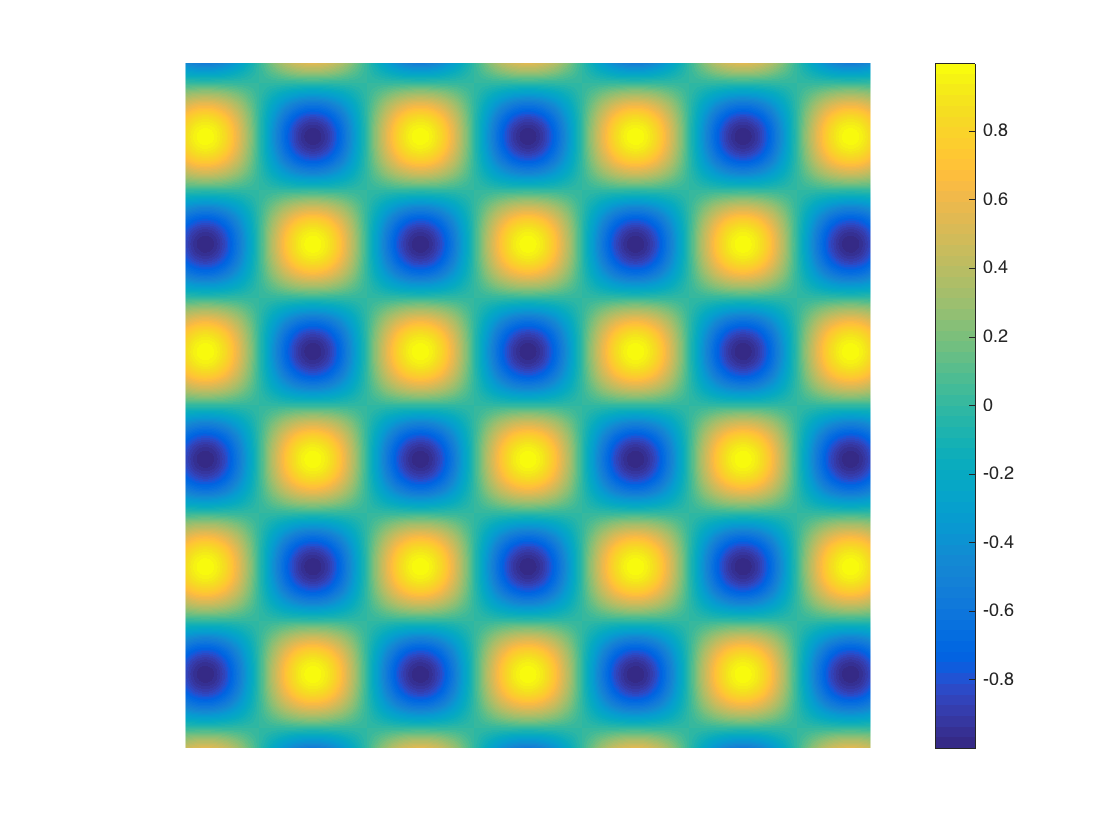
Under these assumptions, the optimal tuning curve in 2D (that maximizes the Fisher Information at all $\bm{\theta}=(\theta_{x},\theta_{y})$) turns out to be the outer product of the sinusoidal waves in $x$ and $y$ directions, which is a rectangular grid-like structure (see figure 1). This optimal solution gaurantees that the variance of estimation at each point within the 2D space is the same for $x$ and $y$ directions (in fact, it is the same for all directions) and is the same for all $\bm{\theta}$ as well.

The details of the analysis for the 2D case is presented in section 6.2.

In this paper, our goal was to show that the grid-like pattern and path integration are closely related. Our analysis suggests that the rectangular grid-like structure is the optimal structure for 2D path integration while the firing field structure for grid cells in MEC are triangular. A recent study [3] has provided theoretical evidence that under a number of reasonable assumptions, triangular grid-like pattern forms the attractor states of the recurrent neural networks. Therefore, it is possible that the neural circuit in entorhinal cortex has converged to a triangular structure because it is an emergent property of the recurrent neural networks.

Fisher Information is based on the local linear estimation paradigm. This implies that it is necessary for the readout mechanism to know the location, $\theta$, in order to measure the small displacements, $\delta\theta$. However, in the problem of path integration, $\theta$ is unknown (in fact, the goal is to integrate $\delta\theta$s to estimate the current $\theta$). As a result, Fisher Information provides a hypothetical variance that is not measurable (observable) in the context of path integration problem.

This problem (that the Fisher Information is not measurable in the context of path integration) can be reduced to the problem of estimating task relevant information in the presence of task irrelevant information. In the case of the path integration problem, task relevant information is $\delta\theta$ while task irrelevant information is $\theta$ itself.

The problem of estimating task relevant information in the presence of task irrelevant information is addressed by Change-based Population Coding (CbPC; [9, 10]). CbPC provides the optimal solution. In our previous work, we addressed this problem in the context of the Bisection task where the location of the bisection array was the task irrelevant information while the offset of the middle bar in the bisection stimulus was the task relevant information.

CbPC’s solution is based on a recurrent neural network that learns a weight matrix that has the following property: There exists a submatrix of the learned recurrent weight matrix that has an eigenvector that is selective to the task relevant information and orthogonal to the task irrelevant information (as well as the dynamical noise). CbPC is described in detail in references [9, 10]. Experimental evidence to support CbPC is still emerging [2, 5, 7].

In this section, we will analyze the 1D case. We will first show that the Fisher information is maximized if all the signal power is given to the eigenvectors that have the smallest eigenvalue (note that each eigenvalue has two corresponding eigenvectors that are oscillatory, are (+/-)90 degrees shifted version of each other (sine and cosine) and have the same (spatial) frequency). We will also show that the optimal tuning curve is oscillatory along the ring and has the same (spatial) frequency as the eigenvectors that carry the signal power. This concludes the analysis for the 1D case.

In this section, we address the 2D case. We assume that the tuning curve for neuron $(i,j)$ (the neuron that is in row $i$ and column $j$) is defined as follows:

where $\theta_{x}$ and $\theta_{y}$ are stimulus coordinates in the $x$ and $y$ directions. We denote the $x$ component of the tuning curve for neuron $(i,j)$ by $f_{x,i}(\theta_{x})$ and the $y$ component by $f_{y,j}(\theta_{y})$. Similar to the 1D case, we assume that, within each direction, the tuning curves of neurons are shifted versions of each other (see 6.1.2).

We also denote the first derivative of $f_{x,i}(\theta)$ at $\theta_{x}$ by $g_{x,i}(\theta)$ and the first derivative of $f_{y,j}(\theta)$ at $\theta_{y}$ by $g_{y,j}(\theta)$; that is, $[\frac{df_{x,i}(\theta^{\prime})}{d\theta^{\prime}}]_{(\theta^{\prime}=\theta)}=g_{x,i}(\theta)$ and $[\frac{df_{y,j}(\theta^{\prime})}{d\theta^{\prime}}]_{(\theta^{\prime}=\theta)}=g_{y,j}(\theta)$.

We also assume that $x$ and $y$ directions in correlation structure in 2D are independent:

We assume that $\bm{C}$ is circulant and symmetric. We denote the inverse of $\bm{C}^{\prime}$ by $\bm{D}^{\prime}$. It is easy to show that $\bm{D}^{\prime}$ can also be decomposed as follows:

Fisher information for one of the variables, say $\theta_{x}$, is as follows :

Based on equation 27 and 26 we have:

Similarly the Fisher Information in the $y$ direction is:

The goal is to maximize the Fisher Information for both $x$ and $y$ directions under the constraint that $\bm{I}_{\theta_{x}}=\bm{I}_{\theta_{y}}$; this is because the variance of estimation should not depend on direction.

The Fisher Information for $x$ and $y$ directions can be written as follows:

where $\bm{f}_{x}=(f_{x,1},f_{x,2},\cdots,f_{x,N})^{T}$, $\bm{g}_{x}=(g_{x,1},g_{x,2},\cdots,g_{x,N})^{T}$, $\bm{f}_{y}=(f_{y,1},f_{y,2},\cdots,f_{y,N})^{T}$, $\bm{g}_{y}=(g_{y,1},g_{y,2},\cdots,g_{y,N})^{T}$ and $\bm{D}$ is the matrix $D_{i,j}$. Note that there is no reason to believe that the shape of the $x$ component of tuning curves is different from the shape of the $y$ components of the tuning curves. Therefore, we assume that they have the same shape.

We denote the eigenvectors of the correlation matrix $\bm{C}$ by $\bm{m}_{i}$ and $\bm{m}^{\prime}_{i}$:

In general, $\bm{g}_{x}(\theta)$ can be written as follows (see section 6.4):

where $K_{i}$ is the (spatial) frequency associated with eigenvector $\bm{m}_{i}$ or $\bm{m}^{\prime}_{i}$. Similar to the 1D case, signal power is fixed, that is:

From equation 33, the $x$ component of the average population activity has the following general form:

Again, we assume that for all $i$, $E_{i}=E^{\prime}_{i}=0$ and $\bm{E}^{\prime\prime}_{i}=\bm{0}$. That is, we are interested in solutions that are symmetric around zero.

We assumed that the shape of the $x$ component of the tuning curves are identical to theshape of the $y$ component of the tuning curves. In other words, if we rotate the $y$ direction by 90 degrees and overlap it with the $x$ direction, then the $x$ component of the average population activity and the $y$ component of the average population activity are identical except that they are shifted versions of each other. As a result:

where $d_{i}=c_{i}+K_{i}\delta\theta$ ($\delta\theta$ denotes the shift between $\bm{f}_{y}(\theta)$ and $\bm{f}_{x}(\theta)$ assuming that one has rotated the $y$ direction by 90 degrees to overlap it with the $x$ direction.)

From equations 30, 33 and 37, we have:

where $\lambda_{i}$ is the eigenvalue associated with eigenvector $\bm{m}_{i}$ or $\bm{m}^{\prime}_{i}$. We assume that $\lambda_{1}=\lambda_{2}>\lambda_{3}=\lambda_{4}>\cdots>\lambda_{N-1}=\lambda_{N}$. Therefore, if we assume that

then similar to the 1D case, the Fisher Information is maximized if all the signal power is focused on the smallest eigenvalue, $\lambda_{N/2}$. Note that this solution also results in $\bm{I}_{\theta_{x},\theta_{y}}=0$, which minimizes the variance $\sigma^{2}_{\theta_{x}}$. Therefore, the maximum Fisher Information is $(\frac{P}{\lambda_{N/2}K_{N/2}})^{2}$ and the minimum variance is $(\frac{\lambda_{N/2}K_{N/2}}{P})^{2}$.

In addition, assuming 39, the optimal solution is the multiplication of two sinusoidal waves (with the same (spatial) frequency $K_{N/2}$) in the $x$ and $y$ directions. In other words, the optimal solution is a rectangular grid-like firing field.

Imagine we have a vector $\bm{z}$ that can be decomposed as follows: $\bm{z}=a\bm{w}+b\bm{w}^{\prime}$ where $\bm{w}$ and $\bm{w}^{\prime}$ are the eigenvectors of a circulant symmetric correlation matrix and have the same spatial frequency $K$. The Fourier transform of $\bm{z}$, $X(\bm{z})$ is as follows: $X(\bm{z})=a+jb$ where $j=\sqrt{-1}$. If we shift (rotate) $\bm{z}$ by $\theta$ and denote it by $\bm{z}^{\prime}$, then according to the shift theorem we have:

In the special case where $a=1$ and $b=0$ (see equation 11), that is, the case where $\bm{z}=\bm{w}$, according to equation 40, $X(\bm{z}^{\prime})=cos(K\theta)+jsin(K\theta)$ and therefore $\bm{z}^{\prime}=cos(K\theta)\bm{w}+sin(K\theta)\bm{w}^{\prime}$.

Another way to intuitively understand the shift theorem is shown in figure 2. Figure 2 shows an example where $K=1$ and $\theta=30$ degrees. Let’s say we want to shift $cos(x)$ (which basically can be regarded as a continuous version of $\bm{w}$) by $\theta=30$ degrees ($K=1$ in this case). If we denote the shifted version by $S(x)$, then $S(x)=cos(\theta)cos(x)+sin(\theta)sin(x)=cos(x-\theta)$. Note that $sin(x)$ is basically the continuous version of $\bm{w}^{\prime}$.

Here we explain equation 33 in more detail .

For $\theta=0$, the first derivative of the population activity, $\bm{g}_{x}(0)$ can be decomposed into the eigenvectors of the correlation matrix as follows:

We ask the following question: what is the equation for $\bm{g}_{x}(\theta)$? We define $\bm{v}_{i}$ as follows:

We denote the 90 degree shifted (rotated) version of $\bm{v}_{i}$ by $\bm{v}^{\prime}_{i}$:

Since $\bm{v}_{i}$ and $\bm{v}^{\prime}_{i}$ are 90 degrees shifted version of each other, we have:

Based on the shift theorem discussed in the previous section, we can shift $\bm{v}_{i}$ by $\theta$ as follows:

where $\bm{x}_{i}$ is the shifted version of $\bm{v}_{i}$ by $\theta$. Note that based on equation 41 and 42 we have:

To shift $\bm{g}_{x}(0)$ by $\theta$ to get $\bm{g}_{x}(\theta)$, we need to shift all its frequencies by $\theta$. Therefore:

Based on equations 47, 45, 42 and 43, it is easy to show that $\bm{g}_{x}(\theta)$ can be written as follows:

In addition, the term ${\bm{g}^{T}_{x}}(\theta)\bm{D}{\bm{g}_{x}}(\theta)=\sum_{i}\frac{T^{2}_{i}}{\lambda_{i}}$ and is independent of $\theta$. Similarly, the term ${\bm{f}^{T}_{x}}(\theta)\bm{D}{\bm{f}_{x}}(\theta)={\bm{f}^{T}_{y}}(\theta_{y})\bm{D}{\bm{f}_{y}}(\theta_{y})=\sum_{i}\frac{T^{2}_{i}}{K^{2}_{i}\lambda_{i}}$, which, again, is independent of $\theta$.

References

- [1] Neil Burgess. Grid cells and theta as oscillatory interference: theory and predictions. Hippocampus, 18(12):1157–1174, 2008.
- [2] David A Crowe, Bruno B Averbeck, and Matthew V Chafee. Rapid sequences of population activity patterns dynamically encode task-critical spatial information in parietal cortex. The Journal of Neuroscience, 30(35):11640–11653, 2010.
- [3] Mark C Fuhs and David S Touretzky. A spin glass model of path integration in rat medial entorhinal cortex. The Journal of Neuroscience, 26(16):4266–4276, 2006.
- [4] Torkel Hafting, Marianne Fyhn, Sturla Molden, May-Britt Moser, and Edvard I Moser. Microstructure of a spatial map in the entorhinal cortex. Nature, 436(7052):801–806, 2005.
- [5] Christopher D Harvey, Philip Coen, and David W Tank. Choice-specific sequences in parietal cortex during a virtual-navigation decision task. Nature, 484(7392):62–68, 2012.
- [6] Steven M Kay. Fundamentals of statistical signal processing, volume i: estimation theory. 1993.
- [7] Valerio Mante, David Sussillo, Krishna V Shenoy, and William T Newsome. Context-dependent computation by recurrent dynamics in prefrontal cortex. Nature, 503(7474):78–84, 2013.
- [8] Bruce L McNaughton, Francesco P Battaglia, Ole Jensen, Edvard I Moser, and May-Britt Moser. Path integration and the neural basis of the’cognitive map’. Nature Reviews Neuroscience, 7(8):663–678, 2006.
- [9] Reza Moazzezi. Change-based population coding. PhD thesis, UCL (University College London), 2011 (available online at: discovery.ucl.ac.uk/1318095/ or http://ethos.bl.uk/OrderDetails.do?uin=uk.bl.ethos.565362).
- [10] Reza Moazzezi and Peter Dayan. Change-based inference for invariant discrimination. Network: Computation in Neural Systems, 19(3):236–252, 2008.
Acknowledgements: This research was partly funded by NSF grant CCF - 1408635.