Exact Electromagnetic Casimir Energy of a Disk Opposite a Plane
Abstract
Building on work of Meixner [J. Meixner, Z. Naturforschung 3a, 506 (1948)], we show how to compute the exact scattering amplitude (or -matrix) for electromagnetic scattering from a perfectly conducting disk. This calculation is a rare example of a non-diagonal -matrix that can nonetheless be obtained in a semi-analytic form. We then use this result to compute the electromagnetic Casimir interaction energy for a disk opposite a plane, for arbitrary orientation angle of the disk, for separations greater than the disk radius. We find that the proximity force approximation (PFA) significantly overestimates the Casimir energy, both in the case of the ordinary PFA, which applies when the disk is parallel to the plane, and the “edge PFA,” which applies when the disk is perpendicular to the plane.
I Introduction
Scattering methods have greatly expanded the range of situations in which one can compute the Casimir energy [1] of quantum electrodynamics. In this approach, one decomposes the path integral representation of the Casimir energy [2] as a log-determinant [3] in terms of a multiple scattering expansion, as was done for asymptotic separations in Ref. [4, 5]. This representation is closely connected to the Krein formula [6, 7, 8] relating the density of states to the scattering matrix for an ensemble of objects. It can also be regarded as a concrete implementation of the perspective emphasized by Schwinger [9] that the fluctuations of the electromagnetic field can be traced back to charge and current fluctuations on the objects.
The scattering method was first developed for general shapes in the context of van der Waals interactions [10]. In planar geometries, the scattering approach yields the Casimir energy in terms of reflection coefficients [11, 12, 13]. By relating the scattering matrix for a collection of spheres [14] or disks [15] to the objects’ individual scattering matrices, Bulgac, Magierski, and Wirzba were also able to use this result to investigate the scalar and fermionic Casimir effect for disks and spheres [16, 17, 18]. A more general formalism, developed in [19, 20, 21], has made it possible to extend these results to other coordinate systems, an approach that is particularly useful for geometries, such as the ones we consider here, with edges and tips [22, 23, 24, 25, 26, 27, 28, 29, 30]. It can also be applied to dilute objects in perturbation theory [31] and extended to efficient, general-purpose numerical calculations [32]; a review and further references can be found in Ref. [33]. In this approach, each object is characterized by its scattering amplitude, also known as the -matrix, which describes its response to an electromagnetic fluctuation. It can therefore be implemented for any object whose -matrix can be calculated using a basis for which an expansion of the free electromagnetic Green’s function exists [34].
For scalar models, the Casimir energy of a disk opposite a plane has been calculated for a general angle between the disk axis and the normal to the plane [35] as the zero-radius limit of an oblate spheroid. Unfortunately, for electromagnetism the wave equation in spheroidal coordinates is not separable. However, Meixner [36] has developed a calculation of diffraction for a disk, using a spheroidal vector basis. By extending this calculation, including an additional subtlety of the case where the azimuthal quantum number is zero, we obtain the -matrix in this basis and use it to calculate the Casimir energy for a perfectly conducting disk opposite a plane. This -matrix is nondiagonal, and the basis in which it is expressed is not orthonormal. Nonetheless, we can implement appropriate conversions to make it amenable to the calculation of the Casimir interaction energy. We apply this method to the case of a disk opposite a plane, including rotations of the disk axis relative to the normal to the plane. This calculation enables us to extend results for conductors with edges in Casimir systems, giving the first example involving a compact object.
II The -matrix
In this section, we calculate the matrix for an infinitely thin and perfectly conducting disk. Here, we build on an earlier calculation for this scattering problem, done by Meixner in his classic paper [36].11 1 An English translation due to N. Sadeh is available from the authors. However, as we will see, that solution was incomplete; we will extend it to obtain the full -matrix, as is required for Casimir calculations.
II.1 Electromagnetic scattering from an infinitely thin conducting disk
We consider a perfectly conducting, infinitely thin disk of radius lying in the plane with the -axis being the symmetry axis of the disk. This idealized case models thin disks, where the thickness of the disk is assumed to be small compared to the wavelength of the electromagnetic field, but large enough for the disk to be perfectly reflecting at the wavelengths of interest. We consider the case of zero temperature, although it is straightforward to extend our calculation to include thermal effects as well.
For a given incoming electric field , we find the corresponding outgoing wave such that the boundary conditions on the disk are satisfied. The standard boundary conditions require that the tangential component of the electric field vanishes on the disk. Were the disk a smooth body without its sharp edge, this condition would be enough to solve the physical scattering problem. However, the sharpness of the infinitely thin disk causes the outgoing field to diverge on the edge. It turns out that there are many outgoing solutions that satisfy the boundary conditions, but diverge at the edge in a way that the integrated electromagnetic energy density is infinite [36]. Such outgoing solutions are nonphysical mathematical solutions of the scattering problem. There is only one solution that diverges slowly enough such that the electromagnetic energy density when integrated is still finite. As a result, this edge condition uniquely fixes the physically correct scattering solution.
The physical scattering problem for an infinitely thin disk can then be formulated in the following way:
- 1.
The fields , obey the Maxwell equations.
- 2.
At large distances, the outgoing wave behaves like an outgoing spherical wave with an angular dependent amplitude.
- 3.
On the disk the field satisfies the boundary conditions .
- 4.
On the edge, the field satisfies the edge condition, i.e. the field diverges slowly enough that the electromagnetic energy of the outgoing field is finite.
Note that the edge condition involves the outgoing field only, because the incoming field does not diverge on the edge. Of course, the scattering problem can equivalently be formulated in terms of the magnetic field .
II.1.1 The Debye potentials
In the following, we use natural units where . Following Meixner [36], we express the and fields in terms of scalar Debye potentials and ,
| (1) | ||||
| (2) |
Here, is the wave number and is the position vector . The Debye potentials solve the scalar wave equation
| (3) |
and therefore the and fields obey the Maxwell equations
| (4) |
To express the boundary conditions for the electric field in terms of the Debye potentials, it is useful to switch to cylindrical coordinates . Due to the axial symmetry of the problem, it is sufficient to consider Debye potentials of the form , where is the conserved azimuthal quantum number. Since the incoming and the outgoing fields have the same dependence, this dependence can be expressed as a Fourier series and considered term by term. Let us therefore substitute into Eq. (1). To eliminate the second derivative with respect to , we use Eq. (3). Then, dropping the common factor of , the and components of the electric field become
| (5) | ||||
| (6) |
Both and have to vanish on the disk. We first solve Eq. (5) for and then Eq. (6) for and get
| (7) | ||||
| (8) |
Eqs. (7) and (8) represent the boundary conditions expressed in terms of the Debye potentials. The functions and depend on and . The boundary conditions are trivially satisfied if . Yet even the trivial solution may violate the edge conditions if the incoming wave is not zero. In general, the physical solution is built out of the trivial solution plus a special solution with nonzero and by exploiting the edge conditions.
Note that if , the right-hand side of Eq. (8) vanishes identically. This case was not considered by Meixner in [36]. As we will see, one must consider this case more carefully to avoid a free undetermined parameter in the equations or to a situation where the edge condition cannot be satisfied at all, resulting in an unphysical solution. We will consider this case later on, but first we formulate the edge conditions.
II.1.2 The edge conditions
Let us now use coordinates appropriate for the scattering problem. The infinitely thin disk can be considered as a limiting case of an oblate spheroid, so that in the following we will use oblate spheroidal coordinates . They are related to the Cartesian coordinates via
| (9) | ||||
| (10) | ||||
| (11) |
where
| (12) |
The surface is then just the disk in the plane having radius and the -axis as a symmetry axis. The center of the disk corresponds to and the edge is described by . We assume that the Debye potentials can be expanded in a Taylor series in terms of and on the edge. The edge conditions, which guarantee that the integrated energy density stays finite, read [36]
| (13) |
To derive Eq. (13), we have to express and as a power series in and , calculate the electromagnetic field using Eqs. (1) and (2), and then integrate the electromagnetic energy density. Then the divergences can be ruled out by imposing Eq. (13).
Let us decompose the Debye potentials into incoming and outgoing parts,
| (14) |
Here, it useful to set , . For on the disk we require
| (15) |
The sum represents the trivial solution in Eq. (7) and (8). The second part of the outgoing Debye potential is then the special solution of the same Eqs. (7) and (8). Note that since the incoming wave fulfills the edge conditions, instead of Eq. (13) it is sufficient to require
| (16) |
for . In the following sections we will derive the solution for , and in terms of spheroidal functions.
II.1.3 Debye potentials in terms of spheroidal functions
There are several coordinate systems in which Eq. (3) can be separated. For example, in spherical coordinates, every solution of Eq. (3) can be expanded in terms of spherical waves , where are the spherical coordinates, and are the spherical quantum numbers, are the Legendre polynomials and are the (incoming or outgoing) spherical Hankel functions. The separation of the wave equation can also be done in spheroidal coordinates . The equivalents of the spherical radial and angular function then are the radial and angular spheroidal functions. The spheroidal wave functions are called Lamé functions and are written as [37, 38]
| (17) | |||
| (18) |
where the first function represents the incoming wave, and the second function the outgoing wave. In contrast to their spherical equivalents, the radial and angular spheroidal functions, and , depend on . In addition, the radial spheroidal function also depends on . Both the angular and radial spheroidal functions become their spherical equivalents as and , and spherical waves can be expanded in terms of spheroidal waves and vice versa. The factors of in the arguments to the spheroidal functions correspond to the oblate case. Finally, we note that, analogously to the spherical case, for even and for odd. In addition is even (odd) in for even (odd).
II.1.4 The first part of the scattered field
Having chosen the appropriate wave basis, let us return to the scattering problem. Since the Maxwell equations (1) are linear in and , it is sufficient to restrict ourselves to the following two cases,
| (19) |
and
| (20) |
for some . In this regard we do not consider incoming plane waves as Meixner in [36], but instead work in a basis of vector spheroidal functions.
The first part, , of the decomposed outgoing potential , (), can then be found straightforwardly. Considering the first case, , , one obtains
| (21) |
For the second case , , the analogous calculation shows that
| (22) |
The derivative in Eq. (22) is taken with respect to . To derive Eqs. (21) and (22), we used Eq. (15).
In general the edge conditions in Eq. (13) will be violated if we substitute into Eq. (13) the first part only. The second part is needed to match the edge conditions. However, for some values of and , the boundary conditions are satisfied by the incoming field alone and the outgoing field vanishes identically. Since for odd, and for even, there is no scattered field for odd in the first case and even in the second. In the next section we will construct for general and .
II.1.5 The second part of the scattered field
The second part of the scattered Debye potential can be expanded in terms of outgoing waves,
| (23) | ||||
| (24) |
To get the functions and , Eqs. (23) and (24) are substituted into Eqs. (7) and (8). Using the orthogonality of the -functions with the normalization convention as in Mathematica and Meixner-Schaefke [37],
| (25) |
and recalling that , we can project the expressions onto the functions, thus eliminating the infinite sums. Then and can be expressed in terms of and as
| (26) | ||||
| (27) |
Here we have explicitly included the indices on and . In addition, we introduced new functions as
| (28) | ||||
| (29) | ||||
| (30) | ||||
| (31) |
with
| (32) |
Note that apart from their indices, the functions , , , , , , and depend on , and in Eqs. (28)–(30) we have also suppressed the dependence on in the functions and . Note also that vanish for odd, and vanish for even. Indeed for odd, the function is odd in . Since it is multiplied by an even function in in Eq. (28) and (29), the integrals for and vanish. Analogously, one verifies the second case.
So far, we have strictly followed Meixner [36], implicitly assuming . For , the functions vanishes identically, whereas the function becomes ill-defined: on the one hand, the integral in Eq. (31) is multiplied by , and on the other hand, the integral itself diverges. The case therefore requires further consideration. For , Eq. (8) simply reads , meaning that is proportional to a -function of . As a result, we find and , where we write the right hand side of Eq. (27) as for the case of .
II.1.6 Calculation of and
In this section we calculate the functions and of Eq. (26) and (27). Then we will be able to determine the second part of the scattered Debye potential, , which, together with the known first part, Eqs. (21) and (22), will eventually lead to the scattered field. For , there are two unknown functions and , which can be calculated from the edge conditions in Eq. (16). There are four edge conditions, but it turns out that that two of them, the second and third of Eq. (16), are always fulfilled, whereas the first and the fourth yield the two equations needed to determine and .
For , as we mentioned at the end of the last section, there are three functions, , and , that need to be determined. At first glance, the system of three unknowns and only two equations seems to be overdetermined. But as we will see, it will be necessary to set , because otherwise the scattered solution will diverge in the center of the disk.
Let us now consider the two following cases for incoming fields, from which all incoming fields can be constructed.
II.1.7 The case ,
Using the fourth edge condition in Eq. (16), we obtain (with )
| (33) |
where is given by Eq. (24). Expressing as in Eq. (27), we get
| (34) |
The sum starts at , since for even. For , the first series vanishes, since , whereas in Eq. (34) has to be replaced by . To satisfy the edge condition, we therefore need , such that vanishes identically.
For , we can express as
| (35) |
The function can be calculated from Eq. (34) as
| (36) |
where the functions and have been defined as
| (37) |
and
| (38) |
Note that the ratio does not depend on .
Unfortunately, the series needed for calculating do not converge if written as in Eqs. (37) and (38). The reason is that the derivative with respect to has been put inside the series. However, evaluating the series with instead of we get well behaved functions of with a well defined derivative at . We will remedy this problem by subtracting the leading term in , which can then be added back in within an analytic computation. The leading order integrals necessary for this subtraction can be computed analytically using Eqs. (119), (120), (121), and (122), as summarized in the Appendix.
The leading order of can be found analytically for any . For small and even we find
| (39) |
and
| (40) |
and for odd we have
| (41) |
and
| (42) |
Subtracting the leading order from the diverging series term by term renders them convergent and numerically evaluable. It is straightforward to extend these results to , since both sums are invariant under .
The remaining edge condition
| (43) |
fixes , which for can be found from Eqs. (21), (23), (26), and (35),
| (44) |
Note the subscript of , which we added for clarity since will have a different functional form in the second case, , , to be considered in the next section. Analogously to Eqs. (37) and (38), here and have been defined as
| (45) |
and
| (46) |
Once again, the series in Eqs. (45) and (46) only converge if the derivative with respect to is taken after the summation over , so we again subtract the leading behavior at small , which is responsible for the divergence. This subtraction can then be added back in as an analytic expression for any . For small and even we obtain
| (47) |
and
| (48) |
and for odd we have
| (49) |
and
| (50) |
while for negative we use that these sums are odd in .
A special case arises for . Eqs. (26) and (27) decouple and strictly speaking we now have to distinguish between in Eq. (26) and in Eq. (27), which are no longer related. Let us consider Eq. (34) for . Since , the left-hand side of Eq. (34) vanishes identically, and so must the right-hand side. Consequently, this implies . Now we are left with two unknowns, and , in Eq. (26). If we keep , the derivative of the potential with respect to will fail to converge for . This would imply a diverging in the center of the disk. This divergence occurs only for and can be cured by setting in Eq. (26). Remarkably, for , the functions vanish at and the field stays finite. Thus we also luckily get rid of an overcounted parameter. The first term and the series over can then be calculated and we find as a function of by exploiting the edge condition in Eq. (43) to obtain
| (51) |
II.1.8 The case ,
The second case , can be treated in a similar way as in the previous section. Using the first edge condition in Eq. (13) and noticing that [see Eq. (22)], we obtain
| (52) |
Expanding in terms of spheroidal waves as in Eq. (23) and expressing as in Eq. (26), we get
| (53) |
As we explained in the previous section, for we have to set , since otherwise will fail to converge at , leading to a diverging electromagnetic field in the middle of the disk. Consequently has to vanish in order to satisfy Eq. (53), meaning that .
Let us now restrict to and express as
| (54) |
The function can be easily calculated from Eq. (53) and is independent of ,
| (55) |
The expansion of the functions and for small is given in the previous section. The remaining edge condition
| (56) |
fixes . Similarly to Eq. (44) we get
| (57) |
Note again the subscript that we added to in order not to confuse the different functional forms in Eq. (44) and (57).
II.2 The T-matrix elements
Having found the complete solution of the scattering problem, we can express our results in terms of the -matrix. The -matrix depends on the product and the quantum numbers and . For large distances from the disk, , the spheroidal modes become spherical modes, which can be of two types: electrical () modes (also called modes) and magnetic () modes (also called modes). This decomposition is a general property of Debye potentials. The potential alone yields a magnetic field with vanishing radial component ( or modes) while the potential corresponds to a vanishing radial component of the electric field ( or modes). Therefore, the -matrix can be split into four submatrices, and . In the following we show how the -matrix can be constructed from the results of the previous sections.
II.2.1 The case ,
As we have seen, the incoming mode generates outgoing fields and . The total potentials and are a superposition of the incoming and outgoing fields and may be written as
| (62) | |||||||||
| (63) |
Let us first consider the case . From Eqs. (21), (23) and (24) we find
| (64) |
and
| (65) |
Note that all functions depend on .
For , the matrix vanishes whereas becomes
| (66) |
For the Casimir interaction at large distances, it is useful to know the behavior of the -matrix at small . For the elements of the and matrices we find for the scaling
| (67) | ||||
| (68) | ||||
| (69) | ||||
| (70) | ||||
| (71) |
For non-vanishing elements, and have to be even. For non-vanishing elements, has to be larger than and even and odd. The matrix elements of order are and .
We now define the vector modes
| (72) |
so that we can write the field in the usual form that defines the -matrix,
| (73) | ||||
showing that our definition agrees with the one used usually for vector spherical waves.
II.2.2 The case ,
The matrices and can be found as in the case before. The T-matrix elements are now defined by
| (74) | |||||||||
| (75) |
We again first consider the case , and obtain
| (76) |
and
| (77) |
For , the matrix vanishes, whereas simplifies to
| (78) |
For the elements of the and matrices we find for at small the scaling
| (79) | ||||
| (80) | ||||
| (81) | ||||
| (82) | ||||
| (83) |
For the non-vanishing elements and have to be odd, and for the non-vanishing elements has to be larger than and odd and even. The only matrix element of is . (Without the contribution from the edge, we would have obtained .)
Finally, with the definitions of Eq. (72), the field can be written as
| (84) | ||||
which corresponds to the usual definition of T-matrix elements.
II.3 Symmetry and unitarity of the -matrix
Because they are not eigenstates of , the modes in Eq. (72) with the same are not orthogonal, and so the -matrix does not have the usual symmetry and unitarity properties in this basis. The asymmetry is particularly pronounced for the case where and : these matrix elements begin at higher order in than the corresponding ones with and . This discrepancy can be traced to the behavior of the coefficient in Eq. (29). Although it appears to be , as we will discuss below, an expansion in yields an expansion of the angular spheroidal in terms of Legendre functions; their orthogonality properties in turn lead to a cancellation of the leading orders in . The true behavior is given by the exact expression for the integral in the case where , given in Eq. (116), which is .
As a result, it will be helpful to convert the -matrix to the basis of spherical vector waves. There exist several normalization conventions; we will use those of Emig et al. [21]. The vector spherical wave functions then read, for an imaginary wave number (which will be useful for the Casimir energy computation below),
| (85) | ||||
| (86) | ||||
| (87) | ||||
| (88) |
where the modified spherical wave functions are
| (89) | |||
| (90) |
Here, is the modified spherical Bessel function of the first kind, and is the modified spherical Bessel function of the third kind.
It is important to note three differences between the definitions of the spherical and spheroidal bases, one of which is nontrivial:
- 1.
The spherical basis has been written in terms of modified radial functions, the conventions for which introduce powers of relative to the ordinary functions with imaginary wave number.
- 2.
The spherical waves have been written in terms of spherical harmonics, which include a factor of compared to the corresponding expression in terms of Legendre functions, the analog of which is used in the spheroidal waves. [For the definition of the factor , see Eq. (32)].
- 3.
The nontrivial difference is the normalization factor of . Because the spheroidal functions are not eigenstates of , no direct analog of this quantity exists in the spheroidal case. (The spheroidal eigenvalue plays a similar role in separation of variables for the scalar wave equation, but that quantity does not yield a corresponding normalization of the vector spheroidal functions.) It is the introduction of this quantity in converting to spherical waves that renders the resulting basis orthonormal. We note also that while the spheroidal basis starts with , the spherical basis starts at .
To convert to the spherical basis, we begin from the expansion of the spheroidal angular functions in terms of Legendre functions,
| (91) |
where the expansion coefficients are obtained via recursion relations [37]. If is even (odd), the summation runs over even (odd) only, and the coefficient is for small . Note that the transformation matrix does not depend on any coordinate. This fact can be used to obtain the transformation formulas for spheroidal waves. At large , the radial spheroidal functions simplify to
| (92) | ||||
| (93) |
Multiplying Eq. (91) by yields the following transformation between scalar waves,
| (94) | ||||
where denotes the spherical Hankel function of type . To verify Eq. (94), we use the asymptotic expansions of at large . One then immediately realizes that Eq. (94) holds for large . Since the transformation matrix does not depend on any coordinate, the relation obtained must also hold at any .
The transformation inverse to Eq. (94) can be found again in the limit of large , in which case the radial functions can be canceled on both sides. Expanding the functions as in Eq. (91) and using the orthogonal relations for the Legendre polynomials similar to those in Eq. (25) for spheroidal angular functions, yields
| (95) |
The inverse matrix is, as expected, the transposed matrix multiplied by normalization factors.
Since the transformation matrix does not depend on any coordinate, the same transformation matrix also transforms between vector waves. We just let the operator and act on Eq. (94), passing through the matrix .
II.4 The - Matrix in the spherical basis
To transform to the spherical basis, we first form a rescaled -matrix, denoted by , in which each matrix element found above is multiplied by a factor of to address the first two differences between the bases listed above. This scaling makes manifest the symmetry in . We then use the following matrix that describes the change of basis,
| (96) | ||||
to convert between the spheroidal basis, indexed by , , and polarization , and the spherical basis, indexed by , , and polarization . Note that the spherical index starts from , while the spheroidal index starts from . The corresponding inverse transformation is given by
| (97) | ||||
We note that the prefactor , which addresses the third difference between the spheroidal and spherical bases listed above, is implemented via the spherical index , which is never zero. We thus obtain the -matrix in the spherical basis as , which has the usual symmetry and unitarity properties.
III The Translation Matrix and the Casimir Energy
Having converted the T-matrix elements to the spherical basis, we are now prepared to evaluate the Casimir energy of a disk that is parallel to an infinite plane, using techniques developed for the sphere-plane problem [39, 40, 21]. In this approach, the Casimir energy is given as
| (98) |
where is the -matrix of the disk in spherical coordinates and combines the reflection coefficient for the plane (see below) and the conversion matrix that expresses spherical vector waves centered at the origin of the disk in terms of planar vector waves centered at the plane. The matrix elements of are given by
| (99) | ||||
where is the distance from the center of the disk to the plane, is the polarization of the plane wave, is for electric modes and for magnetic modes, , is the Fresnel reflection coefficient for scattering from the plane, and
gives the conversion between vector spherical waves and vector plane waves in terms of the associated Legendre functions and its derivative with respect to its argument. For a perfectly conducting plane, for electric and magnetic modes, respectively.
This expression is now suitable for numerical evaluation, which we carry out in Mathematica, using routines for computing spheroidal functions [35, 41] based on the package created by Falloon [42]. This code provides all the necessary spheroidal functions, as well as the expansion coefficients . Since we are carrying out this calculation via a conversion to the spherical basis, we are restricted to configurations with , so that a sphere enclosing the disk does not intersect the plane [21]. Our calculation shows the corresponding numerical instabilities for .
III.1 Rotated disk
The translation matrix elements in Eq. (99) are obtained from the expansion of a plane wave constructed with “pilot vector” in terms of transverse spherical vector modes, which are plane waves with wave vector
| (102) | ||||
| (103) |
By rotating the -axis of the spherical modes to an angle from the normal to the plane, we can obtain the Casimir energy for a disk whose normal is tilted by that angle away from the normal to the plane, allowing us to extend the results found previously for scalar fields [35]. We choose to rotate around the -axis, as shown in Fig. 1. In these coordinates, the pilot vector becomes , and
| (104) |
where
| (105) | ||||
| (106) |

The only change to the calculation is that we now have
| (107) | ||||
| (108) | ||||
where
| (109) | ||||
| (110) | ||||
for , and
| (111) | ||||
| (112) | ||||
for . As in the case of , these expressions are obtained as the dot product of the spherical wave and the corresponding vector spherical harmonic of in the expansion of a plane wave [43, 44]. For any angle , the calculation still requires , so that a sphere enclosing the disk does not intersect the plane. As a result, for , we could consider a disk whose edge is arbitrarily close to the plane. However, as the edge approaches the plane, more partial waves and larger values of are required to accurately compute the infinite sums and integrals.
We note that for , careful attention is needed to avoid problems arising from branch cuts. In particular, Eqs. (109) and (111) can be expressed in terms of , , , , and without the need for any inverse trigonometric functions. Similarly, one must take care to obtain the appropriate analytic continuation of the Legendre functions outside the unit circle.
III.2 Large separations
For , the Casimir energy is dominated by the contribution from large wavelength, corresponding to small . The lowest-order contributions to the -matrix are , , , and . However, does not contribute at lowest order: Since there is no mode in the spherical basis, its effect enters through off-diagonal terms mixing different values of and , which introduce additional powers of . The values of and correspond to the static electric and magnetic dipole responses respectively, and , which agree with previous results [45]. Using the same approach as in the sphere-plane geometry [39], we obtain the Casimir energy in the long-distance limit for as
| (113) |
Higher-order terms are more difficult to obtain, because they require resummation of the infinite sums in , , , and at the appropriate order in .
IV Results
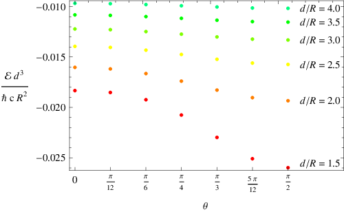
Figure 2 shows the Casimir energy for a perfectly conducting disk of radius and a perfectly conducting plane, as a function of the rotation angle for different separations . To facilitate the comparison between difference separation distances, the energies have been scaled by a factor of , since a decay is predicted by the proximity force approximation (PFA). The plots range from , when the disk is parallel to the plane, to , when the disk is perpendicular to the plane, and from to . We note that at these separations, the full energy for is still significantly smaller in magnitude than the prediction of the PFA,
| (114) |
which on this graph would correspond to a value of , independent of . In these calculations, we have truncated the numerical sums after and used the interval for the integral over , and we have checked that the results are not sensitive to these choices. (The dimensionless ratio must be a function of the dimensionless quantities and .)
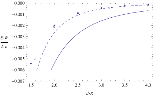

For the case where the disk is parallel to the plane, Fig. 3 shows a comparison of our result for the Casimir energy and the PFA prediction. We also show numerical results obtained by using the fluctuating-surface-current method [32].22 2 This calculation is implemented in the SCUFF-EM package, available from http://GitHub.com/HomerReid/SCUFF-EM . The two exact methods agree well, demonstrating that the magnitude of the energy is significantly smaller than the PFA prediction. For the case when the disk is perpendicular to the plane, the Casimir energy is shown in Fig. 4. We see that the result is also smaller than the “edge PFA,” based on the result for a half-plane with a sharp edge opposite an infinite plane [25],
| (115) |
V Conclusions
Building on Meixner’s analysis of diffraction from a disk [36], we have constructed the full scattering -matrix for the scattering of light from a perfectly conducting disk, which we have then expressed in a vector spherical wave basis, a calculation that requires particular attention to finite contributions arising from singular terms in the channel. This result represents one of the few cases of a non-diagonal -matrix that can be computed exactly in closed form. The scattering approach then allows us to use this information to obtain Casimir interaction energies for systems such as the disk-plane geometry we have considered here, for arbitrary orientations of the disk. This approach is particularly valuable for configurations where edge effects are important, such as the case where the disk is perpendicular to the plane, since there one cannot use a gradient expansion for gently curved surfaces [46, 47]. We have found that the PFA result significantly overestimates the Casimir energy at intermediate distances, as does the “edge PFA” based on the result for a half-plane.
While conversion to the vector spherical basis facilitates the consideration of different rotation angles, it limits the calculation to , to ensure that a sphere enclosing the disk does not intersect the plane. In order to allow , one must consider instead the vector spheroidal basis, which is not orthonormal. Since the scattering method relies on a mode expansion of the free Green’s function, it cannot be applied directly to the spheroidal basis; as a result, an important direction for future work is to generalize the scattering method to include this case.
Acknowledgements.
This work is based on preliminary studies of the scattering problem for a disk by Alexej Weber in an earlier stage of this project. His contribution is acknowledged. We thank G. Bimonte, R. L. Jaffe, M. Kardar, and M. Krüger for helpful discussions, and M. T. H. Reid for carrying out comparisons with the methods of Ref. [32]. N. G. was supported in part by the National Science Foundation (NSF) through grant PHY-1520293.Appendix A Useful Integrals
Here we collect useful integrals, obtained from [48, 49, 50]. For , we have the closed-form integrals
| (116) | ||||
and
| (117) | ||||
where the normalization factor is given by
| (118) |
We can also simplify the leading-order subtractions using the integrals
| (119) |
and
| (120) |
where from these results we can also obtain
| (121) |
and
| (122) |
using integration by parts and recurrence relations for Legendre functions.
References
- [1] H. B. G. Casimir, Proc. K. Ned. Akad. Wet. 51, 793 (1948).
- [2] T. Emig, A. Hanke, R. Golestanian, and M. Kardar, Phys. Rev. Lett. 87, 260402 (2001).
- [3] O. Kenneth and I. Klich, Phys. Rev. Lett. 97, 160401 (2006).
- [4] R. Balian and B. Duplantier, Ann. Phys. (N.Y.) 104, 300 (1977).
- [5] R. Balian and B. Duplantier, Ann. Phys. (N.Y.) 112, 165 (1978).
- [6] M. G. Krein, Mat. Sborn. (NS) 33, 597 (1953).
- [7] M. G. Krein, Sov. Math.-Dokl. 3, 707 (1962).
- [8] M. S. Birman and M. G. Krein, Sov. Math.-Dokl. 3, 740 (1962).
- [9] J. Schwinger, Lett. Math. Phys. 1, 43 (1975).
- [10] D. Langbein, Theory of Van der Waals attraction (Springer-Verlag, Berlin, Heidelberg, 1974).
- [11] E. I. Kats, Sov. Phys. JETP 46, 109 (1977).
- [12] M. T. Jaekel and S. Reynaud, J. Physique I 1, 1395 (1991).
- [13] A. Lambrecht, P. A. Maia Neto, and S. Reynaud, New J. Phys. 8, 243 (2006).
- [14] M. Henseler, A. Wirzba, and T. Guhr, Ann. Phys. (N.Y.) 258, 286 (1997).
- [15] A. Wirzba, Phys. Rep. 309, 1 (1999).
- [16] A. Bulgac and A. Wirzba, Phys. Rev. Lett. 87, 120404 (2001).
- [17] A. Bulgac, P. Magierski, and A. Wirzba, Phys. Rev. D 73, 025007 (2006).
- [18] A. Wirzba, J. Phys. A: Math. Theor. 41, 164003 (2008).
- [19] T. Emig, N. Graham, R. L. Jaffe, and M. Kardar, Phys. Rev. Lett. 99, 170403 (2007).
- [20] O. Kenneth and I. Klich, Phys. Rev. B 78, 014103 (2008).
- [21] S. J. Rahi, T. Emig, N. Graham, R. L. Jaffe, and M. Kardar, Phys. Rev. D 80, 085021 (2009).
- [22] H. Gies and K. Klingmuller, Phys. Rev. Lett. 97, 220405 (2006).
- [23] A. Weber and H. Gies, Phys. Rev. D80, 065033 (2009).
- [24] M. F. Maghrebi, S. J. Rahi, T. Emig, N. Graham, R. L. Jaffe, and M. Kardar, Proc. Nat. Acad. Sci. 108, 6867 (2011).
- [25] N. Graham, A. Shpunt, T. Emig, S. J. Rahi, R. L. Jaffe, and M. Kardar, Phys. Rev. D81, 061701 (2010).
- [26] N. Graham, A. Shpunt, T. Emig, S. J. Rahi, R. L. Jaffe, and M. Kardar, Phys. Rev. D83, 125007 (2011).
- [27] D. Kabat, D. Karabali, and V. Nair, Phys. Rev. D81, 125013 (2010a).
- [28] D. Kabat, D. Karabali, and V. Nair, Phys. Rev. D82, 025014 (2010b).
- [29] N. Graham, Phys. Rev. D87, 105004 (2013).
- [30] E. N. Blose, B. Ghimire, N. Graham, and J. Stratton-Smith, Phys. Rev. A 91, 012501 (2015).
- [31] K. A. Milton and J. Wagner, J. Phys. A: Math. Theor. 41, 155402 (2008).
- [32] M. T. H. Reid, A. W. Rodriguez, J. White, and S. G. Johnson, Phys. Rev. Lett. 103, 040401 (2009).
- [33] D. Dalvit, P. Milonni, D. Roberts, and F. da Rosa, eds., Geometry and Material Effects in Casimir Physics-Scattering Theory (Springer-Verlag, Berlin, Heidelberg, 2011), pp. 129–174.
- [34] C.-T. Tai, Dyadic Green Functions in Electromagnetic Theory (IEEE Press, New York, 1994).
- [35] T. Emig, N. Graham, R. L. Jaffe, and M. Kardar, Phys. Rev. A 79, 054901 (2009).
- [36] J. Meixner, Z. Naturforschung 3a, 506 (1948).
- [37] J. W. Meixner and R. W. Schäfke, Mathieusche Funktionen und Sphäroidfunktionen (Springer-Verlag, Berlin, 1954).
- [38] C. Flammer, Spheroidal Wave Functions (Stanford University Press, Stanford, CA, 1957).
- [39] T. Emig, J. Stat. Mech. p. P04007 (2008).
- [40] P. A. Maia Neto, A. Lambrecht, and S. Reynaud, Phys. Rev. A 78, 012115 (2008).
- [41] N. Graham and K. D. Olum, Phys. Rev. D 72, 025013 (2005).
- [42] P. E. Falloon, P. C. Abbott, and J. B. Wang, J. Phys. A: Math. Gen. 36, 5477 (2003).
- [43] D. Varshalovich, A. Moskalev, and V. Khersonsky, Quantum Theory of Angular Momentum: Irreducible Tensors, Spherical Harmonics, Vector Coupling Coefficients, 3-j Symbols (World Scientific, Hackensack, NJ, 1988).
- [44] A. Forrow and N. Graham, Phys. Rev. A86, 062715 (2012).
- [45] R. Friedberg, American Journal of Physics 61, 1084 (1993).
- [46] C. D. Fosco, F. C. Lombardo, and F. D. Mazzitelli, Phys. Rev. D84, 105031 (2011).
- [47] G. Bimonte, T. Emig, R. L. Jaffe, and M. Kardar, Europhys. Lett. 97, 50001 (2012).
- [48] A. Erdélyi, W. Magnus, F. Oberhettinger, and F. G. Tricomi, Higher Transcendental Functions (MacGraw-Hill, New York, 1953).
- [49] M. Abramowitz and I. A. Stegun, Handbook of Mathematical Functions With Formulas, Graphs, and Mathematical Tables (U.S. government printing office, Washington, 1972).
- [50] I. S. Gradshteyn and I. M. Ryzhik, Table of Integrals, Series, and Products (Academic Press, San Diego, 1994), 5th ed.