The Standard Model of particle physics provides viable parameterisation for all subatomic data to date. The most striking feature of the Standard Model, augmented by right–handed neutrinos that are required by the neutrino data, is the embedding of its chiral spectrum in three chiral 16 representations of $SO(10)$. Heterotic–string models give rise to spinorial 16 representations in the perturbative spectrum and therefore preserve the $SO(10)$ embedding of the Standard Model states [1, 2].

Recently, a possible signal has been reported by the ATLAS [3] and CMS [4] collaborations that would indicate a clear deviation from the Standard Model. Both experiments reported early indications for enhancement of di–photon events with a resonance at 750GeV, and generated substantial interest [5]. A plausible explanation for this enhancement is obtained if the resonant state is assumed to be a Standard Model singlet state, and the production and decay are mediated by heavy vector–like quark and lepton states [5, 6, 7]. These characteristics arise naturally in heterotic–string models that allow for a light extra $Z^{\prime}$ [8].

We note that the construction of heterotic–string models that allow for a light $Z^{\prime}$ is highly non–trivial [9, 10, 11] . The reason being that the extra family universal $U(1)$ symmetries that are typically discussed in the string–inspired literature tend to be anomalous and are therefore broken near the string scale [12]. The relevant symmetries tend to be anomalous due to the symmetry breaking pattern $E_{6}\rightarrow SO(10)\times U(1)_{\zeta}$, induced at the string level by the Gliozzi–Scherk–Olive (GSO) projection [13]. In ref. [11] we used the spinor–vector duality property of $Z_{2}\times Z_{2}$ orbifolds [14, 15] to construct a string derived model with anomaly free $U(1)_{\zeta}$, thus enabling it to remain unbroken down to low scales.

An additional constraint imposed by the heterotic–string is that the gauge, as well as the gravitational, couplings are unified at the string scale [16]. Since the early nineties, much of the research on the phenomenology of supersymmetric grand unified theories has been motivated by the observation that the unification of the gauge couplings in SUSY GUTs is compatible with the measured gauge coupling data at the electroweak scale, provided that we assume that the spectrum between the two scales consists of that of the Minimal Supersymmetric Standard Model (MSSM) [17]. Following Witten we may assume that the string and GUT scales may coincide in the framework of $M$–theory [18].

A vital question therefore is to examine what is the corresponding situation in the heterotic–string derived $Z^{\prime}$ models. We find that, quite remarkably, in the $Z^{\prime}$ models the compatibility of gauge coupling unification with the data at the electroweak scale is identical to the case of the MSSM. We further show that effects arising from heavy thresholds may push the supersymmetric spectrum beyond the reach of the LHC, while maintaining the agreement with the gauge coupling data. We show that the string inspired model can indeed account for the observed signal and discuss the feasibility of obtaining viable scalar mass spectrum.

While further data from the LHC did did not substantiate the observation of the di–photon excess [19, 20], a di–photon excess is a general signature of this class of $Z^{\prime}$ models. The results presented in this paper are therofore relevant for continuing $Z^{\prime}$ searches at the LHC.

The difficulty in constructing heterotic–string models with light $Z^{\prime}$ symmetries arises due to the breaking of the observable $E_{6}$ symmetry in the string constructions by discrete Wilson lines to $SO(10)\times U(1)_{\zeta}$. Application of the symmetry breaking at the string level results in the projection of some states from the physical spectrum. The consequence is that $U(1)_{\zeta}$ is in general anomalous in the string vacua, and cannot remain unbroken to low scales. The extra $U(1)$ symmetry which is embedded in $SO(10)$, and is orthogonal to the Standard Model weak hypercharge, is typically broken at the high scale to generate sufficiently light neutrino masses. Flavour non–universal $U(1)$ symmetries must be broken above the deca–TeV scale to avoid conflict with Flavour Changing Neutral Current (FCNC) constraints [21].

The string derived model of ref. [11] was constructed in the free fermionic formulation [22] of the heterotic–string. The details of the construction, the massless spectrum of the model and its superpotential are given in ref. [11] and will not be repeated here. We review here the properties of the model that are relevant for the anomaly free extra $Z^{\prime}$ symmetry.

The model utilises the spinor–vector duality symmetry that was observed in the space of fermionic $Z_{2}\times Z_{2}$ orbifold compactifications [14, 15]. The spinor vector duality operates under exchange of the total number of spinorial $({16}\oplus\overline{16})$ representations of $SO(10)$ with the total number of vectorial $10$ representations. For every string vacuum with a $\#_{1}$ of $({16}\oplus\overline{16})$ representations and $\#_{2}$ of 10 representations there is a dual vacuum in which $\#_{1}\leftrightarrow\#_{2}$. The understanding of this duality is facilitated by considering the vacua in which the $SO(10)\times U(1)_{\zeta}$ symmetry is enhanced to $E_{6}$. The chiral representations of $E_{6}$ are the $27$ and $\overline{27}$ and their decomposition under $SU(10)\times U(1)_{\zeta}$ is

where the subscript denotes the $U(1)_{\zeta}$ charge. Thus, the string vacua with $E_{6}$ symmetry are self–dual with respect to the spinor–vector duality, i.e. in these vacua $\#_{1}(16\oplus\overline{16})=\#_{2}(10)$. In this case $U(1)_{\zeta}$ is anomaly free by virtue of its embedding in $E_{6}$. There exist a discrete Wilson line that reduce $E_{6}$ symmetry to $SO(10)\times U(1)_{\zeta}$ with $\#_{1}(16\oplus\overline{16})~\&~\#_{2}(10)$, and a corresponding discrete Wilson line with $\#_{2}(16\oplus\overline{16})~\&~\#_{1}(10)$ [15].

The string vacua with enhanced $E_{6}$ symmetry correspond to heterotic–string vacua with $(2,2)$ worldsheet supersymmetry. We can realise the $E_{6}$ symmetry by breaking the ten dimensional untwisted gauge symmetry to $SO(8)^{4}$ [14]. One of the $SO(8)$ factors is reduced further to $SO(2)^{4}$ and the $E_{6}$ symmetry is generated from additional sectors in the string vacua. In parallel to the spectral flow operator on the supersymmetric side of the heterotic–string that maps between different spacetime spin representations, there exists a spectral flow operator on the bosonic side. In the vacua with enhanced $E_{6}$ symmetry the spectral flow operator exchanges between the spinorial and vectorial components in the $E_{6}$ representations. The spectral flow operator is the $U(1)$ generator of the $N=2$ worldsheet supersymmetry on the bosonic side of the heterotic–string. In the vacua with broken $E_{6}$ symmetry, the $N=2$ worldsheet supersymmetry on the bosonic side is broken and the spectral flow operator induces the map between the spinor–vector dual vacua. The picture was extended to other internal CFTs in ref. [23].

The class of $Z_{2}\times Z_{2}$ vacua affords another possibility. It is possible to construct self–dual vacua with $\#_{1}(16\oplus\overline{16})=\#_{2}(10)$, without enhancing the gauge symmetry to $E_{6}$. This is the case if the different components of the $E_{6}$ representations are obtained from different fixed points of the $Z_{2}\times Z_{2}$ orbifold. The spectrum then forms complete $E_{6}$ representations, but the gauge symmetry is not enhanced to $E_{6}$ and remains $SO(10)\times U(1)_{\zeta}$, with $U(1)_{\zeta}$ being anomaly free due to the fact that the chiral spectrum still forms complete $E_{6}$ multiplets. It is important to note that this is possible only because the spinorial and vectorial $SO(10)$ representations are obtained from different fixed points. Obtaining the $16$ and $(10+1)$ components at the same fixed point necessarily implies that the gauge symmetry is enhanced to $E_{6}$.

The construction of ref. [11] utilises the classification methods developed in ref. [24] for type IIB string and in ref. [25] for heterotic–string vacua with unbroken $SO(10)$ gauge group. The heterotic–string classification was extended to vacua with the Pati–Salam and flipped $SU(5)$ subgroups of $O(10)$ in refs. [26] and [27], respectively. In this method a space of the order of $10^{12}$ is spanned and models with specific phenomenological characteristics can be extracted. The string vacuum with anomaly free $U(1)_{Z^{\prime}}$ is obtained by first trawling a self–dual $SO(10)$ model with six chiral families and subsequently breaking the $SO(10)$ symmetry to the Pati–Salam subgroup [11]. The chiral spectrum of the models forms complete $E_{6}$ representations, whereas the additional vector–like multiplets may reside in incomplete multiplets. This is in fact an additional important property of the string, which affects compatibility with the gauge coupling data. The complete massless spectrum of the model was presented in ref. [11]. Spacetime vector bosons are obtained solely from the untwisted sector and generate the observable and hidden gauge symmetries, given by:

The $E_{6}$ combination,

is anomaly free whereas the orthogonal combinations of $U(1)_{1,2,3}$ are anomalous. The complete massless spectrum of the string model and the charges under the gauge symmetries are given in ref. [11]. Tables 1 and 2 show a glossary of the states in the model and their charges under the $SU(4)\times SO(4)\times U(1)_{\zeta}$ group factors, where we adopt the notation of ref. [8]. The sextet states are in vector–like representations with respect to the Standard Model, but are chiral under $U(1)_{\zeta}$. Thus, if $U(1)_{\zeta}$ is part of an unbroken $U(1)_{Z^{\prime}}$ combination down to low scales, it protects the sextets, and corresponding bi–doublets, from acquiring a mass above the $U(1)_{Z^{\prime}}$ breaking scale. The model also contains vector–like states that transform under the hidden $SU(2)^{4}\times SO(8)$ group factors, with charges $Q_{\zeta}=\pm 1$ or $Q_{\zeta}=0$.

As noted from table 1 the string model contains the Higgs representations required to break the non–Abelian Pati–Salam gauge symmetry [28]. These are ${\cal H}=F_{R}$ and $\bar{\cal H}$, being a linear combination of the four $\bar{F}_{R}$ fields. The decomposition of these fields under the Standard Model group is given by:

The suppression of the left–handed neutrino masses favours the breaking of the Pati–Salam (PS) gauge symmetry at the high scale [29, 30]. The possibility of breaking the PS symmetry at a low scale was considered in refs. [31, 32]. Here we will take the PS breaking scale to be in the vicinity of the string scale or slightly below. The VEVs of the heavy Higgs fields that break the PS gauge group leave an unbroken $U(1)_{Z^{\prime}}$ symmetry given by

that may remain unbroken down to low scales provided that $U(1)_{\zeta}$ is anomaly free. Cancellation of the anomalies requires that the additional vector–like quarks and leptons, that arise from the $10$ representation of $SO(10)$, as well as the $SO(10)$ singlet in the $27$ of $E_{6}$, remain in the light spectrum. The three right–handed neutrino states are neutral under the low scale gauge symmetry and receive mass of the order of Pati–Salam breaking scale. The spectrum below the PS breaking scale is displayed schematically in table 3. The spectrum is taken to be supersymmetric down to the TeV scale. As in the MSSM, compatibility of gauge coupling unification with the experimental data requires the existence of one vector–like pair of Higgs doublets, beyond the number of vector–like triplets. This is possible in the free fermionic heterotic–string models due to the stringy doublet–triplet splitting mechanism [33]. We allow also for the possibility of light states that are neutral under the low scale gauge group. In ref. [8] we showed that the string model contains all the ingredients to account for the LHC di–photon excess, provided that the vector–like pairs of colour triplets and electroweak doublets receive a mass of the order of the TeV scale. This explanation is particularly appealing if the $U(1)_{Z^{\prime}}$ remains unbroken down to low scales. In this case the mass of the vector–like states can only be generated by the VEV of the $SO(10)$ singlets $S_{i}$ and/or ${\phi_{1,2}}$ that breaks the $U(1)_{Z^{\prime}}$ gauge symmetry. In this scenario the scale of the di–photon excess fixes the scale of the $U(1)_{Z^{\prime}}$ breaking to be of the order of the TeV scale. It is therefore of interest to examine the compatibility of this picture with the gauge coupling data.

In this section we analyse the compatibility of gauge coupling unification in the string inspired model with the low energy gauge coupling data, where we may assume that the unification scale is either at the GUT or string scales [18]. We examine the case in which the PS symmetry is broken at the string scale as well as the case in which is broken at an intermediate scale. We take the following values for the input parameters at the $Z$–mass scale [34]:

We also include the top quark mass of $M_{t}\sim 173.5$ GeV [34] and the Higgs boson mass of $M_{H}\sim 125$ GeV [35] in our analysis. String unification implies that the Standard Model gauge couplings are unified at the heterotic–string scale. The one–loop renormalisation group equations (RGEs) for the gauge couplings are given by

where $b_{i}$ are the one–loop beta–function coefficients, $\Delta_{i}^{\left(\mbox{\tiny{total}}\right)}$ represents corrections two–loop and mixing effects, and $k_{i}=\{1,1,5/3\}$ for $i=3,2,1$. The analysis is most revealing at the one–loop level. Therefore, for the most part we limit our exposition to the one–loop investigation and give an estimate of the higher order corrections, which do not affect the overall picture. We obtain algebraic expressions for $\sin^{2}\theta_{W}\left(M_{Z}\right)$ and $\alpha_{3}\left(M_{Z}\right)$ by solving the one–loop RGEs. In our analysis, we initially assume the full spectrum of the $Z^{\prime}$ model between the unification scale, $M_{X}$, and the $Z$–boson scale, $M_{Z}$, and treat all perturbations as effective threshold terms. At the unification scale we have

where $k_{1}={5}/{3}$ is the canonical $SO(10)$ normalisation. We initially study the case in which the PS symmetry is broken at the string scale. In this case the expression for $\left.\sin^{2}\theta_{W}\left(M_{Z}\right)\right|_{\overline{MS}}$ takes the general form

with $\left.\alpha_{3}\left(M_{Z}\right)\right|_{\tiny{\overline{MS}}}$ having a similar form with corresponding $\Delta^{\alpha_{3}}$ corrections. Here $\Delta_{Z^{\prime}}$ is the one–loop contribution from the states of the $Z^{\prime}$ model between the unification scale and the $Z$–boson mass scale. $\Delta_{\mbox{\tiny{L.T.}}}$ are corrections from the light thresholds, which consist of the light supersymmetric thresholds; the Higgs and the top mass thresholds; and the mass thresholds of the heavy vector–like matter states in the $Z^{\prime}$ model. The last term,

includes the two–loop; kinetic mixing; Yukawa couplings and scheme conversion corrections. These corrections are found to be small and do not affect the overall picture. These effects can be absorbed into modifications of the light thresholds, which in any case are not fixed and can be varied. For $\sin^{2}\theta_{W}\left(M_{Z}\right)$ we obtain

where $M_{i}$ are the light mass thresholds and $\alpha=\alpha_{\mbox{\tiny{e.m.}}}\left(M_{Z}\right)$. Similarly for $\alpha_{3}\left(M_{Z}\right)$, we have:

The predictions for gauge coupling observables at the $Z$–scale can therefore be seen to correspond to $0^{th}$ order predictions consisting of the first lines of eqs. (3.6) and (3.7) plus the threshold corrections due to the decoupling of the different particles at their mass thresholds. The values of the beta function coefficients of these light thresholds are shown in table 4. The $0^{th}$ order coefficients are given by

Hence, the $b_{i}^{\mbox{\tiny{$Z^{\prime}$}}}$ are identical to the $b_{i}^{\mbox{\tiny{MSSM}}}$ up to a common shift by 3, arising from the vector–like colour triplets and electroweak doublets. As the $0^{th}$ order predictions for $\sin\theta(M_{Z})$ and $\alpha_{3}(M_{Z})$ only depend on the differences of the beta function coefficients, the zeroes order predictions are identical to those that are obtained in the MSSM.

The corrections due to the light thresholds are given by

It is noted from eqs. (3.8) and (3.9) that if the vector–like colour triplets are degenerate in mass with the vector–like electroweak doublets, then their threshold corrections exactly cancel. In that case the predictions for $\sin^{2}\theta_{W}(M_{Z})$ and $\alpha_{3}(M_{Z})$ coincide exactly with those of the MSSM. The exact masses of these states depend of course on the details of their couplings to the $Z^{\prime}$ breaking VEV. Allowing for mass splitting of the order of a few TeV may be compensated by contributions from the supersymmetric states. Imposing the experimental limits on the supersymmetric particles and allowing for such mass differences figure 1 shows a scatter plot of $\sin^{2}\theta_{W}(M_{Z})$ and $\alpha_{3}(M_{Z})$, where the masses of the supersymmetric particles are varied independently.

$\alpha_{{}_{S}}(M_{Z})$

$$\sin^{2}\theta_{W}(M_{Z})$$

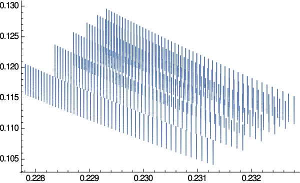
Next we study the predictions for the gauge coupling parameters with Pati–Salam breaking at an intermediate energy scale $M_{PS}$. The gauge symmetry is $SU(4)_{C}\times SU(2)_{L}\times SU(2)_{R}\times U(1)_{\zeta}$, and $SU(3)_{C}\times SU(2)_{L}\times U(1)_{Y}\times U(1)_{Z^{\prime}}$, above and below the intermediate Pati--Salam breaking scale, respectively. The weak hypercharge is given by⁵⁵ 5 $U(1)_{C}=3U(1)_{B-L}/2;~U(1)_{\hat{C}}=U(1)_{C}/\sqrt{3}$.

with $k_{C}=6$. When solving the RGEs for the low scale predictions we have to distinguish the running above and below the intermediate breaking scale. The RGEs and beta function coefficients below the symmetry breaking scale coincide with those of the $Z^{\prime}$ model discussed above. Above the symmetry breaking scale the spectrum differs from the standard Pati–Salam model due to the anomaly cancellation requirement of $U(1)_{\zeta}$. To ensure that $U(1)_{\zeta}$ is anomaly free, all the additional states above the intermediate breaking scale have to be vector–like with respect to $U(1)_{\zeta}$. The Pati–Salam model contains an additional sextet field required for the missing–partner–like mechanism that gives heavy mass to the heavy Higgs states [36]. Hence, anomaly cancellation with respect to $U(1)_{\zeta}$ demands another sextet in the spectrum with opposite $U(1)_{\zeta}$ charge. Similarly, the spectrum above the intermediate symmetry breaking scale contains two bi–doublet states with opposite $U(1)_{\zeta}$ charges, whereas only one pair of Higgs doublets remain below the intermediate scale. The beta function coefficients above the intermediate breaking scale are therefore

which also takes into account the contribution of the heavy Higgs states, and $b_{2}^{\mbox{\tiny{PS}}},~b_{\mbox{\tiny{R}}}^{\mbox{\tiny{PS}}}$ are the beta function coefficients of $SU(2)_{L}~,SU(2)_{R}$, respectively. The effect of the intermediate symmetry breaking scale is to add correction terms to eqs. (3.6) and (3.7), given by

Restricting to experimentally viable predictions for $\sin^{2}\theta_{W}(M_{Z})$ and $\alpha_{3}(M_{Z})$, and varying $M_{PS}$ and a common SUSY breaking scale $M_{SUSY}$, while keeping $M_{X}=1.1\times 10^{16}{\rm GeV}$ we obtain a relation between $M_{PS}$ and $M_{SUSY}$ which is displayed in figure 2. From the figure we note that reducing the intermediate Pati–Salam symmetry breaking scale pushes the supersymmetric thresholds beyond the LHC reach. Nevertheless, the $Z^{\prime}$ breaking scale remains at the TeV scale as the contribution of the extra vector–like colour triplets is canceled by that of the extra vector–like doublets.

The effects of the extra vector–like states above the Pati–Salam breaking scale may also mitigate the unification of the gauge coupling closer to the perturbative heterotic–string scale. Assuming an additional pair of sextet fields, fixing $M_{SUSY}\sim 2{\rm TeV}$ and $M_{X}\sim 1\times 10^{17}{\rm GeV}$, we note that by varying the PS breaking scale we obtain viable predictions for $\sin^{2}\theta_{W}(M_{Z})$ and $\alpha_{3}(M_{Z})$. These results are displayed in figure 3.

Split bi–doublet and sextet multiplets naturally appear in string models due to the stringy doublet–triplet stringy mechanism, which depends on the assignment of boundary conditions in the basis vectors that break the $SO(10)$ symmetry to the Pati–Salam subgroup [33]. The model of [11] contains three such pairs of untwisted sextets, and one additional pair from the twisted sectors, whereas there is no excess of vector–like bi–doublets. This is the case because the model of [11] utilises symmetric boundary conditions with respect to the internal manifold, whereas a model with asymmetric assignment would generate corresponding extra bi–doublets. The string models therefore contain all the ingredients to naturally produce agreement with a di–photon excess as well as agreement with the gauge coupling data at the electroweak scale.

We may also consider the case of the left–right symmetric model in which the $SO(10)$ symmetry is broken to $SU(3)\times U(1)_{C}\times SU(2)_{L}\times SU(2)_{R}$. We assume that $U(1)_{\zeta}$ charges admit the $E_{6}$ embedding. In this case the heavy Higgs states consists of the pair ${\cal N}\left({\bf 1},{\bf\frac{3}{2}},{\bf 1},{\bf 2},{\bf\frac{1}{2}}\right),~{\bar{\cal N}}\left({\bf 1},-{\bf\frac{3}{2}},{\bf 1},{\bf 2},-{\bf\frac{1}{2}}\right).$ The VEV along the electrically neutral component leaves unbroken the Standard Model gauge group and the $U(1)_{Z^{\prime}}$ combination in eq. (2.2). We remark, however, that in the free fermionic LRS models [37] the $U(1)_{\zeta}$ charges do not admit the $E_{6}$ embedding and we will argue in [38] that in a large class of string models such construction is not possible. Here, we consider such models as purely field theory models and study the effect on the low scale gauge coupling parameters. Above the symmetry breaking scale the spectrum coincides with that of table 3 with the right–handed fields arranged into doublet representations of $SU(2)_{R}$. Additionally, the spectrum contains the heavy Higgs states and a pair of Higgs bi–doublets with opposite $U(1)_{\zeta}$ charges. Crucially, here, the intermediate symmetry breaking does not require the existence of coloured states in the interval between $M_{R}$ and $M_{X}$, which may be incorporated in non–minimal extensions. Consequently, the beta function coefficients above the intermediate symmetry breaking scale $M_{R}$ are

whereas the $b^{\mbox{\tiny{$Z^{\prime}$}}}_{i}$ below the intermediate breaking scale coincide with those given above. Here, $b_{2}^{\mbox{\tiny{R}}}$ is the beta function coefficient of $SU(2)_{L}$; $b_{\mbox{\tiny{R}}}^{\mbox{\tiny{R}}}$ is that of $SU(2)_{R}$; and $b^{\mbox{\tiny{R}}}_{\mbox{\tiny{$\hat{C}$}}}$ is that of the normalised $U(1)_{C}$ generator. The effect of the intermediate scale symmetry breaking is to add correction terms for $\sin^{2}\theta_{W}(M_{Z})$ and $\alpha_{3}(M_{Z})$ given by

As seen in figure 4 similar to the PS case the effect of the intermediate scale corrections to $\sin^{2}\theta_{W}(M_{Z})$ and $\alpha_{3}(M_{Z})$ is to shift the common SUSY threshold beyond the reach of the LHC. The figures should be viewed as illustrative, indicating the substantial impact that a low scale $Z^{\prime}$ may have on the anticipated signatures at accessible energy scales. This should be contrasted with the corresponding intermediate scale models [39], in which the impact of the intermediate scale corrections is milder.

In the low energy regime the superpotential [11] provides different interaction terms of the singlet fields $S_{i}$ and $\zeta_{i}$ which can be extracted from table  3, among them we have

All these terms may comply with the di–photon excess reported by both the ATLAS and CMS experiments with a resonance around 750 GeV described by either the singlets $S_{i}$ or $\zeta_{i}$. Indeed, the presence of vector-like quarks, which is natural in heterotic-string models, facilitates the production of these states at the LHC. In the following discussion we will consider the most simple and economic scenario in order to highlight the effects of the vector-like coloured states $D,\bar{D}$ and their role in the explanation of the di–photon excess. For this reason we assume that the resonance is reproduced by exchange of one of the singlet $S_{i}$ and we ignore the contribution of the $\zeta_{i}$ fields and of the coupling $SH\bar{H}$. The real scalar component of one of the $S_{i}$ superfields acquires a VEV $v_{S}$ and breaks the extra $U(1)_{Z^{\prime}}$ symmetry thus providing the mass of the $Z^{\prime}$ gauge boson and of the $D,\bar{D}$ field through the coupling $\lambda_{D}$ in the superpotential (4.1). Provided $v_{S}$ around the TeV scale, the mass of the singlet $S_{i}$, of the vector-like states $D,\bar{D}$ and of the $Z^{\prime}$ lay in the TeV ballpark thus establishing a intimate relationship between the 750 GeV di–photon resonance and the presence of an additional spontaneously broken $U(1)_{Z^{\prime}}$ gauge symmetry. Interestingly this can also be probed at the LHC in the lepto-production channel [41, 32]. Moreover, as we have already stated, in order to reproduce the di–photon excess it is enough to consider the impact of the vector-like coloured superfields $D,\bar{D}$ only. Therefore we assume $\lambda\equiv\lambda^{3ii}_{D}$ and we neglect all the other couplings. The fermionic components of $D_{i}$ and $\bar{D}_{i}$ can be rearranged into three Dirac spinors $\psi_{D_{i}}$, while the scalar components will provide six complex scalars $\tilde{D}_{j}$. The corresponding interaction Lagrangian can be parameterised as

References

- [1] D.J. Gross, J.A. Harvey, E.J. Martinec and R. Rohm, Nucl. Phys. B267 (1986) 75.
- [2] P. Candelas, G.T. Horowitz, A. Strominger and E. Witten, Nucl. Phys. B258 (1985) 46.
- [3] ATLAS Collaboration, G. Aad et al, ATLAS–CONF–2015–081.
- [4] CMS Collaboration, S. Chatrchyan et al, CMS PAS EXO–15–004.
- [5]
For a partial list see e.g.:
K. Harigaya and Y. Nomura, arXiv:1512.04850;
A. Pilaftsis, arXiv:1512.04931;
R. Franceschini et al., arXiv:1512.04933;
S. Di Chiara, L. Marzola and M. Raidal, arXiv:1512.04939;
S.D. McDermott, P. Meade and H. Ramani, arXiv:1512.05326;
J. Ellis et al, arXiv:1512.05327;
R.S. Gupta et al, arXiv:1512.05332;
Q.H. Cao et al, arXiv:1512.05542; arxiv:1512.08441;
A. Kobakhidze et al, arXiv:1512.05585;
R. Martinez, F. Ochoa and C.F. Sierra, arXiv:1512.05617;
J.M. No, V. Sanz and J. Setford, arXiv:1512.05700;
W. Chao, R. Huo and J.H. Yu, arXiv:1512.05738;
L. Bian, N. Chen, D. Liu and J. Shu, arXiv:1512.05759;
J. Chakrabortty et al, arXiv:1512.05767;
A. Falkowski, O. Slone and T. Volansky, arXiv:1512.05777;
D. Aloni et al, arXiv:1512.05778;
W. Chao, arXiv:1512.06297;
S. Chang, arXiv:1512.06426;
R. Ding, L. Huang, T. Li and B. Zhu, arXiv:1512.06560;
X.F. Han, L. Wang, arXiv:1512.06587;
T.F. Feng, X.Q. Li, H.B. Zhang and S.M. Zhao, arXiv:1512.06696;
F. Wang, L. Wu, J.M. Yang and M. Zhang, arXiv:1512.06715;
F.P. Huang, C.S. Li, Z.L. Liu and Y. Wang, arXiv:1512.06732;
M. Bauer and M. Neubert, arXiv:1512.06828;
M. Chala, M. Duerr, F. Kahlhoefer and K. Schmidt-Hoberg, arXiv:1512.06833;
S.M. Boucenna, S. Morisi and A. Vicente, arXiv:1512.06878;
C.W. Murphy, arXiv:1512.06976;
G.M. Pelaggi, A. Strumia and E. Vigiani, arXiv:1512.07225;
J. de Blas, J. Santiago and R. Vega-Morales, arXiv:1512.07229;
A. Belyaev et al, arXiv:1512.07242;
P.S.B. Dev and D. Teresi, arXiv:1512.07243;
K.M. Patel and P. Sharma, arXiv:1512.07468;
S. Chakraborty, A. Chakraborty and S. Raychaudhuri, arXiv:1512.07527;
W. Altmannshofer et al, arXiv:1512.07616;
B.C. Allanach, P.S.B. Dev, S.A. Renner and K. Sakurai, arXiv:1512.07645;
N. Craig, P. Draper, C. Kilic and S. Thomas, arXiv:1512.07733;
J.A. Casas, J.R. Espinosa and J.M. Moreno, arXiv:1512.07895;
L.J. Hall, K. Harigaya and Y. Nomura, arXiv:1512.07904;
A. Salvio and A. Mazumdar, arXiv:1512.08184;
J. Cao, C. Han, L. Shang, W. Su, J. M. Yang and Y. Zhang, Phys. Lett. B755 (2016) 456;
J. Cao, L. Shang, W. Su, F. Wang and Y. Zhang, arXiv:1512.08392;
J. Cao, L. Shang, W. Su, Y. Zhang and J. Zhu, Eur. Phys. Jour. C76 (2016) 5;
K. Das and S. K. Rai, Phys. Rev. D93 (2016) 095007;
F. Wang et al, arXiv:1512.08434;
X. J. Bi et al., arXiv:1512.08497;
F. Goertz, J.F. Kamenik, A. Katz and M. Nardecchia, arXiv:1512.08500;
P.S.B. Dev, R.N. Mohapatra and Y. Zhang, arXiv:1512.08507;
S. Kanemura, N. Machida, S. Odori and T. Shindou, arXiv:1512.09053;
I. Low and J. Lykken, arXiv:1512.09089;
A.E.C. Hernández, arXiv:1512.09092;
Y. Jiang, Y.Y. Li and T. Liu, arXiv:1512.09127;
K. Kaneta, S. Kang and H. S. Lee, arXiv:1512.09129;
L. Marzola et al, arXiv:1512.09136;
X.F. Han et al, arXiv:1601.00534;
W. Chao, arXiv:1601.00633;
T. Modak, S. Sadhukhan and R. Srivastava, arXiv:1601.00836;
F.F. Deppisch et al, arXiv:1601.00952;
I. Sahin, arXiv:1601.01676;
R. Ding, Z.L. Han, Y. Liao and X. D. Ma, arXiv:1601.02714;
T. Nomura and H. Okada, arXiv:1601.04516;
X.F. Han, L. Wang and J.M. Yang, arXiv:1601.04954;
D.B. Franzosi and M.T. Frandsen, arXiv:1601.05357;
U. Aydemir and T. Mandal, arXiv:1601.06761;
J. Shu and J. Yepes, arXiv:1601.06891;
J. Kawamura and Y. Omura, arXiv:1601.07396;
L. Aparicio, A. Azatov, E. Hardy and A. Romanino, arXiv:1602.00949;
R. Ding et al, arXiv:1602.00977;
K.J. Bae, M. Endo, K. Hamaguchi and T. Moroi, arXiv:1602.03653;
F. Staub et al., arXiv:1602.05581;
M. Badziak, M. Olechowski, S. Pokorski and K. Sakurai, arXiv:1603.02203;
R. Franceschini et al, arXiv:1604.06446;
K.J. Bae, C.R. Chen, K. Hamaguchi and I. Low, arXiv:1604.07941;
B.G. Sidharth et al, arXiv:1605.01169. - [6]
B. Dutta et al, arXiv:1512.05439;
B. Dutta et al, arXiv:1601.00866 [hep-ph];
A. Karozas, S.F. King, G.K. Leontaris and A.K. Meadowcroft, arXiv:1601.00640;
S.F. King and R. Nevzorov, arXiv:1601.07242;
T. Li, J.A. Maxin, V.E. Mayes and D.V. Nanopoulos, arXiv:1602.01377;
Y. Hamada, H. Kawai, K. Kawana and K. Tsumura, arXiv:1602.04170;
N. Liu, W. Wang, M. Zhang and R. Zheng, arXiv:1604.00728;
H.P. Nilles and M.W. Winkler, arXiv:1604.03598. - [7]
J.J. Heckman, arXiv:1512.06773;
L.A. Anchordoqui et al, arXiv:1512.08502; arXiv:1603.08294;
L.E. Ibanez and V. Martin-Lozano, arXiv:1512.08777;
M. Cvetic, J. Halverson and P. Langacker, arXiv:1512.07622; arXiv:1602.06257;
E. Palti, arXiv:1601.00285;
P. Anastasopoulos and M. Bianchi, arXiv:1601.07584;
G.K. Leontaris and Q. Shafi, arXiv:1603.06962. - [8] A.E. Faraggi and J. Rizos, Eur. Phys. Jour. C76 (2016) 170.
- [9] A.E. Faraggi and D.V. Nanopoulos, Mod. Phys. Lett. A6 (1991) 61.
- [10]
J. Pati, Phys. Lett. B388 (1996) 532;
A.E. Faraggi, Phys. Lett. B499 (2001) 147;
A.E. Faraggi and M. Thormeier, Nucl. Phys. B624 (2002) 163;
C. Coriano, A.E. Faraggi and M. Guzzi, Eur. Phys. Jour. C53 (2008) 421;
A.E. Faraggi and V. Mehta, Phys. Rev. D84 (2011) 086006; Phys. Rev. D88 (2013) 025006;
P. Athanasopoulos, A.E. Faraggi and V. Mehta, Phys. Rev. D89 (2014) 105023. - [11] A.E. Faraggi and J. Rizos, Nucl. Phys. B895 (2015) 233.
- [12]
G.B. Cleaver and A.E. Faraggi, Int. J. Mod. Phys. A14 (1999) 2335;
A.E. Faraggi and J.C. Pati, Nucl. Phys. B526 (1998) 21;
A.E. Faraggi, Phys. Lett. B426 (1998) 315. - [13] F. Gliozzi, J. Scherk and D.I. Olive, Nucl. Phys. B122 (1977) 253.
- [14]
A.E. Faraggi, C. Kounnas and J. Rizos, Nucl. Phys. B774 (2007) 208;
Nucl. Phys. B799 (2008) 19;
C. Angelantonj, A.E. Faraggi and M. Tsulaia, JHEP 1007, (2010) 004. - [15]
T, Catelin–Jullien, A.E. Faraggi, C. Kounnas and J. Rizos, Nucl. Phys. B812 (2009) 103;
A.E. Faraggi, I. Florakis, T. Mohaupt and M. Tsulaia, Nucl. Phys. B848 (2011) 332. - [16]
P.H. Ginsparg, Phys. Lett. B197 (1987) 139;
V.S. Kaplunovsky, Nucl. Phys. B307 (1988) 145. - [17]
S. Dimopoulos, S. Raby and F. Wilczek, Phys. Rev. D24 (1981) 1681;
M.B. Einhorn and D.R.T. Jones, Nucl. Phys. B196 (1982) 475;
J. Elllis, S. Kelley and D.V. Nanopoulos, Phys. Lett. B249 (1990) 441;
P. Langacker and M. Luo, Phys. Rev. D44 (1991) 817;
U. Amaldi, W. de Boer and H. Furstenau, Phys. Lett. B260 (1991) 447;
A.E. Faraggi and B. Grinstein, Nucl. Phys. B422 (1994) 3. - [18] E. Witten, Nucl. Phys. B471 (1996) 135.
- [19] ATLAS Collaboration, G. Aad et al, ATLAS-CONF-2016-059.
- [20] CMS Collaboration, S. Chatrchyan et al, CMS-PAS-EXO-16-027.
- [21] G. Cleaver, A.E. Faraggi, D.V. Nanopoulos and T. ter Veldhuis, Int. J. Mod. Phys. A16 (2001) 3565.
- [22]
H. Kawai, D.C. Lewellen, and S.H.-H. Tye,
Nucl. Phys. B288 (1987) 1;
I. Antoniadis, C. Bachas, and C. Kounnas, Nucl. Phys. B289 (1987) 87;
I. Antoniadis and C. Bachas, Nucl. Phys. B289 (1987) 87. - [23] P. Athanasopoulos, A.E. Faraggi and D. Gepner, Phys. Lett. B735 (2014) 357.
- [24] A. Gregori, C. Kounnas and J. Rizos, Nucl. Phys. B549 (1999) 16.
- [25]
A.E. Faraggi, C. Kounnas, S.E.M. Nooij and J. Rizos, Nucl. Phys. B695 (2004) 41;
A.E. Faraggi, C. Kounnas and J. Rizos, Phys. Lett. B648 (2007) 84. - [26] B. Assel, K. Christodoulides, A.E. Faraggi, C. Kounnas and J. Rizos, Phys. Lett. B683 (2010) 306; Nucl. Phys. B844 (2011) 365.
- [27]
A.E. Faraggi, J. Rizos and H. Sonmez, Nucl. Phys. B886 (2014) 202;
H. Sonmez, arXiv:1603.03504. - [28] J. Pati and A. Salam, Phys. Rev. D10 (1974) 275.
- [29]
I. Antoniadis, G.K. Leontaris and J. Rizos,
Phys. Lett. B245 (1990) 161;
G.K. Leontaris and J. Rizos, Nucl. Phys. B554 (1999) 3;
K. Christodoulides, A.E. Faraggi and J. Rizos, Phys. Lett. B702 (2011) 81. - [30]
A.E. Faraggi, Phys. Lett. B245 (1990) 435;
A.E. Faraggi and E. Halyo, Phys. Lett. B307 (1993) 311;
C. Coriano and A.E. Faraggi, Phys. Lett. B581 (2004) 99. - [31]
A. Kuznetsov and M. Mikheev, Phys. Lett. B329 (1994) 295;
G. Valencia and S. Willenbrock, Phys. Rev. D50 (1994) 6843;
R.R. Volkas, Phys. Rev. D53 (1996) 2681;
R. Foot, Phys. Lett. B420 (1998) 333. - [32] A.E. Faraggi and M. Guzzi, Eur. Phys. Jour. C75 (2015) 537.
- [33] A.E. Faraggi, Nucl. Phys. B428 (1994) 111; Phys. Lett. B520 (2001) 337.
- [34] K.A. Olive et al. [Particle Data Group Collaboration], Chin. Phys. C38 (2014) 090001.
- [35]
S. Chatrchyan et al. [CMS Collaboration], JHEP 1306, (2013) 081;
G. Aad et al. [ATLAS Collaboration], Phys. Lett. B716 (2012) 1. - [36] I. Antoniadis and G. Leontaris, Phys. Lett. B216 (1989) 333.
- [37]
G.B. Cleaver, A.E. Faraggi and C. Savage,
Phys. Rev. D63 (2001) 066001;
G.B. Cleaver, D.J. Clements and A.E. Faraggi Phys. Rev. D65 (2002) 106003. - [38] J. Ashfaque, A.E. Faraggi R. Tatar, work in progress.
- [39] K.R. Dienes and A.E. Faraggi, Nucl. Phys. B457 (1995) 409.
- [40] A.D. Martin, W.J. Stirling, R.S. Thorne and G. Watt, Eur. Phys. Jour. C63 (2009) 189.
- [41] C. Coriano, A.E. Faraggi and M. Guzzi, Phys. Rev. D78 (2008) 015012.
- [42]
E. Gabrielli et al,
Phys. Lett. B756 (2016) 36;
A. Salvio, F. Staub, A. Strumia and A. Urbano, JHEP 1603, (2016) 214. - [43] U. Ellwanger, C. Hugonie and A. M. Teixeira, Phys. Rep. 496 (2010) 1.
- [44] M. Quiros and J.R. Espinosa, hep-ph/9809269.
- [45] I. Antoniadis, J. Ellis, J. Hagelin and D.V. Nanopoulos Phys. Lett. B231 (1989) 65.
- [46]
A.E. Faraggi, D.V. Nanopoulos and K. Yuan,
Nucl. Phys. B335 (1990) 347;
A.E. Faraggi, Phys. Lett. B278 (1992) 131; Nucl. Phys. B387 (1992) 239;
G.B. Cleaver, A.E. Faraggi and D.V. Nanopoulos, Phys. Lett. B455 (1999) 135;
A.E. Faraggi, E. Manno and C. Timirgaziu, Eur. Phys. Jour. C50 (2007) 701. - [47] L. Bernard, A.E. Faraggi, I. Glasser, J. Rizos and H. Sonmez, Nucl. Phys. B868 (2013) 1.
- [48]
A.E. Faraggi, Phys. Lett. B326 (1994) 62; Phys. Lett. B544 (2002) 207;
E. Kiritsis and C. Kounnas, Nucl. Phys. B503 (1997) 117;
A.E. Faraggi, S. Forste and C. Timirgaziu, JHEP 0608, (2006) 057;
P. Athanasopoulos, A.E. Faraggi, S. Groot Nibbelink and V.M. Mehta, JHEP 1604, (2016) 038.